Abstract
The detection of gravitational waves in 2015 ushered in a new era of gravitational wave (GW) astronomy capable of probing the strong field dynamics of black holes and neutron stars. It has opened up an exciting new window for laboratory and space tests of Einstein’s theory of classical general relativity (GR). In recent years, two interesting proposals have aimed to reveal the quantum nature of perturbative gravity: (1) theoretical predictions on how graviton noise from the early universe, after the vacuum of the gravitational field was strongly squeezed by inflationary expansion; (2) experimental proposals using the quantum entanglement between two masses, each in a superposition (gravitational cat, or gravcat) state. The first proposal focuses on the stochastic properties of quantum fields (QFs), and the second invokes a key concept of quantum information (QI). An equally basic and interesting idea is to ask whether (and how) gravity might be responsible for a quantum system becoming classical in appearance, known as gravitational decoherence. Decoherence due to gravity is of special interest because gravity is universal, meaning, gravitational interaction is present for all massive objects. This is an important issue in macroscopic quantum phenomena (MQP), underlining many proposals in alternative quantum theories (AQTs). To fully appreciate or conduct research in these exciting developments requires a working knowledge of classical GR, QF theory, and QI, plus some familiarity with stochastic processes (SPs), namely, noise in quantum fields and decohering environments. Traditionally a new researcher may be conversant in one or two of these four subjects: GR, QFT, QI, and SP, depending on his/her background. This tutorial attempts to provide the necessary connective tissues between them, helping an engaged reader from any one of these four subjects to leapfrog to the frontier of these interdisciplinary research topics. In the present version, we shall address the three topics listed in the title, excluding gravitational entanglement, because, despite the high attention some recent experimental proposals have received, its nature and implications in relation to quantum gravity still contain many controversial elements.
1. Matching the Main Themes with Different Readers’ Backgrounds and Needs
We assume that three different communities of readers share a common goal: to understand the newly important topics of graviton noise and gravitational decoherence in relation to gravitational radiation. These readers may come from different backgrounds, such as (A) classical general relativity, specializing in gravitational wave physics or astronomy. They are curious about how experiments like those conducted by LIGO/LISA can be useful for detecting these effects; (B) quantum field or particle theorists who know field theory but are interested in understanding how quantum noise arises and how these stochastic quantities and related effects can impact potentially observable gravitational quantum phenomena; (C) atomic–optical and condensed matter physicists with working knowledge in open quantum systems and quantum information. They are curious about how this expertise can be applied to the investigation of gravitating systems, possibly even touching on quantum gravity issues.
As remarked in the abstract section, graviton physics invokes GR and QFT, gravitational decoherence invokes GR (we do not consider alternative quantum or gravity theories here), and concepts and techniques of open quantum systems (OQSs). Thus, we can see some crisscrossing of the four ingredients: classical gravity (GR), quantum field (QFT), quantum information (QI), and quantum noise (OQS). In the environment-induced decoherence (QI) conceptual scheme, the noise in the graviton field (GR + QFT) acting as an environment to a quantum system induces decoherence of that quantum system. Thus, quantum–classical transition or correspondence is one of our underlying themes. A full range of coherent topics would start from graviton noise, i.e., fluctuations in the quantized (perturbative) gravitational field, and ending with classical gravitational radiation [1], with radiation reaction considerations. This issue has been addressed for scalar and electromagnetic fields so we shall only mention the conceptual pathways here without going into the details.
After this dissection of the two main themes, readers with different backgrounds can see from the Table of Contents the sections or topics they can skip over and the ones that are more useful for their specific purposes.
Content-wise, we start with gravitational wave physics based on perturbation theory (not fluctuations) off of the Minkowski spacetime. (Note the often-ignored yet important difference between perturbations, which obey deterministic equations of motion, and fluctuations/noises that are stochastic variables). Then we quantize the field where spin 2 gravitons appear. We show that each of the two polarizations obeys an equation of the same form as a massless minimally coupled scalar field. We then analyze Green’s functions and the quantum states of this field. We point out that the two most important Green’s functions for our problems are the retarded and Hadamard functions, with the latter being responsible for noise in the quantum field. We discuss four types of Gaussian quantum states: the vacuum, coherent, squeezed vacuum, and squeezed coherent states. We then argue how to go from the quantum field theory to classical radiation theory, via the coherent state, but hasten to point out not to ignore the important quantum features of coherent states when considering the quantum to classical transition. Hereby, we show how noise and fluctuations can be gleaned from a full quantum field theoretical treatment, discouraging any ad hoc additions, as these would violate the intrinsic structure of the theory, such as is evident in fluctuation-dissipation relations.
As a tutorial, we will bypass the explanation of motivations for specific topics and the extensive background literature, and dive directly into developing the necessary ingredients. We shall refer to textbooks and research papers from which our material is derived, where readers can find broader coverage or further details. However, a broader perspective is necessary to avoid misinterpretations of the larger issues. Therefore, in the final section, we discuss how the topics presented here relate to graviton physics, the quantum nature of gravity, and quantum gravity. These are longstanding issues of fundamental significance, but they have gained new relevance with the additional consideration of quantum information issues and the stochastic properties of quantum fields. The focus is on the difference between the physics of gravitons, which are the quantized weak perturbations of spacetime, and quantum gravity, which refers to theories concerning the basic constituents and fundamental structures of spacetime. Gravitons have been present since the manifold structure of spacetime began to take shape, as they are the quanta of its weak perturbations and are, in principle, detectable at today’s low energies. In contrast, quantum gravity is non-perturbative, background-independent, and involves physics at the Planck energy and above. The consequences of quantum gravity can only be deduced indirectly from observations of the early universe or quantum processes near black holes below the Planck energy. We aim to help readers understand the significant conceptual divide and technical challenges between graviton physics and quantum gravity. Specifically, recent proposals for laboratory experiments that leverage quantum information considerations, such as entanglement, can aid understanding of the quantum nature of perturbative gravity or graviton physics but have little relevance to quantum gravity proper.
Stylistically, we try to present just enough materials from each base, in some cases starting from familiar textbook materials, to enable uninitiated readers to comprehend these interdisciplinary subjects with some economy in the effort. For this reason, our presentation may seem crisp in some places, compact in others, and even pedestrian to those familiar with certain topics, but less so to others, but there is no sacrifice of rigor or accuracy. We hope that the ‘pedestrian bridges’ we build between these scenic attractions are smoothly paved enabling curious explorers or serious researchers to stroll easily across them while enjoying the pleasant views.
2. Gravitational Waves: Metric Perturbations of Minkowski Spacetime
Here, we include a short review of the classical gravitational wave, adapted from the classic “Gravitation” by Misner, Thorne, and Wheeler (MTW) [2].
2.1. Linear Perturbations
We consider a simpler case where the metric perturbations are excited in background Minkowski spacetime, whose metric, denoted by , has the signature . Suppose, we write the full metric as
where the metric perturbation is assumed to be small . The condition gives
The split of the full metric into the background and perturbation is not unique even if the background spacetime is Minkowskian due to the gauge choices of . If we make an infinitesimal change to the coordinate system,
then in this new coordinate system, the metric is given by
and the metric perturbations will take a new form,
Apparently, the metric perturbations depend on the choice of the coordinate system. In other words, the metric perturbations are gauge-dependent. Thus, we may choose a suitable gauge to simplify the calculations associated with the metric perturbations.
To the first-order metric perturbation, the Christoffel symbols are given by the expression
and then the Riemann tensor has the following form:
Consequently, the Ricci tensor and the Ricci scalar R are given by
if we keep terms up to the first order in , where the trace of is .
In the Einstein equation,
the form of the Einstein tensor, defined by , implies that it may be convenient to introduce the trace-reversed form of the metric perturbations as follows
with . By the trace-reversed metric perturbations, the Einstein tensor is greatly simplified into
Now, we see the advantage of using trace-reversed metric perturbations. If we choose the Lorenz gauge , then the Einstein equation reduces to
It has a form of the wave equation driven by the source on the right-hand side. Note that, when arriving at this form, we do not need the traceless condition , as it is usually applied to fix the degrees of freedom in the polarization tensor below.
The trace-reversed metric perturbations transform according to
Thus, under the gauge transformation (13), the Riemann tensor does not change,
That is, it is gauge-invariant in Minkowski spacetime.
2.2. Polarization Tensors and Degrees of Freedom
Since the metric perturbation is a symmetric tensor of rank two, it has 10 independent components. The Lorenz gauge gives four constraints so that the independent degrees of freedom drop to six. However, if the graviton is massless, we expect that only two physical degrees of freedom remain.
A particularly convenient choice of gauge in the context of gravitational radiation is to pick , . Together with , they form the transverse–traceless (TT) gauge, and reduce the degrees of freedom in down to two. If we write in the following generic form,
then in the absence of the source, Equation (12) implies , with a plane-wave solution . If we suppose that the perturbations propagate along the z direction, then we have two independent polarization tensors, , each of which takes a particular simple form:
Thus, the metric perturbations propagate as transverse waves at the speed of light, with polarizations described by (16). It is of interest to note that even though the “amplitude” of the wave is small, the gravitational wave can induce quite a substantial curvature for sufficiently short wavelength modes.
In the transverse–traceless gauge, there is no difference between and due to , so we will remove the overhead bar hereafter. Clearly, the gravitational wave polarizes in a way different from the light waves. Since the metric perturbation changes the physical length scales, it is easier to see its effects via the relative distance. For example, we may arrange a bunch of test particles to form a circle on the x–y plane and examine how their relative positions change when a plane gravitational wave traveling along the z direction passes through them. Suppose each particle is initially at rest with an initial four-velocity , then the geodesic deviation between the neighboring geodesics of the test particles is described by
for the Minkowski background, where gives the relative position orthogonal to the four-velocity . The neighboring test particles will be displaced from the circle, according to the polarization of the waves, as shown in Figure 1. For example, if the incoming wave has the + polarization, the circle of particles will be distorted over time into ellipses with varying eccentricities. The major and minor axes of these ellipses will align with the x and y axes.
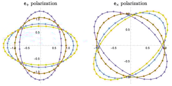
Figure 1.
The physical effects of polarizations of the metric perturbations. Different colors correspond to different times.
2.3. Quantized Gravitational Wave in Minkowski Spacetime
Similar to quantizing the electromagnetic wave, we may quantize the gravitational wave and promote to an operator in a plane-wave expansion,
where labels two independent polarization tensors for each mode , with , and , and its Hermitian conjugate is the standard creation and annihilation operator, satisfying the following: .
Since the wave three-vector is not limited to the z-direction, it is not straightforward to write down the polarization tensors right off hand. A useful observation is that the polarization tensors in (16) can be written as dyadic products of the usual polarization unit vectors and along the x and y axes as follows:
with the triad satisfying the orthogonal relations, and , with , such that
Thus, for a general , if we have two mutually orthogonal unit vectors, and , and they are also orthogonal to , then we can construct two polarization tensors in the same way as shown in (19).
There is no unique way to determine and due to the cylindrical symmetry about in their orthogonality conditions with . We may start with an arbitrary but fixed unit three-vector , not collinear with , to find and by
It is straightforward to check that forms a set of orthonormal bases for the spatial section of Minkowski spacetime. The arbitrariness of is a manifestation of the aforementioned symmetry.
It will be convenient to put the above triad into a covariant expression,
with, for example, and , where the Greek letters run from 0 to 3 while the Latin letters range from 1 to 3. Here, we implicitly assume a preferred frame in which the four-velocity and . This implies that, along with the triad, we can use this four-velocity to form a tetrad with for Minkowski spacetime with the handedness condition
where is the Levi–Civita tensor in Minkowski spacetime, which gives 1 if , , , form even permutations of 0, 1, 2, 3, and for odd permutations, and 0 if any two of the tensor indices are the same. Then, we can generalize the orthogonality condition of the tetrad from (22) to the following:
which will be valid in any frame. The completeness condition of the tetrad is then formulated as
Recall that the innermost subscript in the notation of the polarization vector is the label of the polarization vector, not the tensor indices. The polarization tensors then follow accordingly.
It appears that from this point, we can treat the quantized gravitational wave and its quanta, gravitons, in a manner similar to the quantized electromagnetic field and photons, and further discuss their physical effects due to interactions with other matter fields using standard quantum field theory techniques. However, it has been argued that if higher-order contributions are systematically included, such a quantized theory is not renormalizable due to the dimensional nature of the coupling strength, namely the Newton constant. Thus, we will restrict ourselves to the low-energy regime, limited by some energy cutoff scale that depends on the configuration at hand, and treat the quantized gravitational wave theory as an effective field theory.
Keeping the above consideration in mind, we will discuss the nature of the quantized gravitation wave in some of the well-known Gaussian states and the corresponding two-point functions of the graviton. Among the latter, the retarded Green’s function and the Hadamard function will be the building blocks to discuss the quantum effects of linearized gravity.
3. Quantum Field Theory: Green’s Functions and Graviton States
The simplest two-point function of the free quantized gravitational field is the Wightman function, defined by
where is the expectation value with respect to a given pure state of the graviton, but when the state is mixed, the notation corresponds to the trace average with respect to that state. In addition, here we assume that . If not, we simply replace with or with in the definitions of Green’s functions. Hereafter, we will use the Heisenberg picture. Apart from the tensor indices, the superscript in a notation like specifies the type of field the Green’s function is associated with, and the subscript gives the kind of Green’s function. If the subscript contains a zero, it means the associated field is a free field; otherwise, it is an interacting field. Occasionally, we will put an additional superscript to indicate the state of the graviton. For example, shows that this is a Wightman function of the free graviton in its thermal state. This myriad of superscripts and subscripts will be useful when we deal with interacting systems.
The retarded Green’s function is given by
with , and being the Heaviside unit step function. It will be shown later that Green’s function respects the causal structure of Minkowski spacetime and relays the causal influence of the source point to the field point x. It is of interest to note that due to the standard commutation relation, the retarded Green’s function of the free quantized gravitational wave is state-independent, so it will have the same form for all quantum states of the graviton. In the context of the in–in or the influence functional formalism outlined in Appendix A, this retarded Green’s function is often termed the dissipation kernel.
Another Green’s function that often accompanies the retarded Green’s function is the Hadamard function, also called the noise kernel, which is the expectation value of the anti-commutator of the free field operator :
In contrast to its retarded Green’s function counterpart, it is, in general, state-dependent, and nonzero even for the space-like interval between x and .
Finally, in the in–out formalism or the context of graviton scattering, we often come across the Feynman propagator , which is given by the expectation value of the time-ordered free field operator :
where denotes time ordering in the sense of for any pair of bosonic operators and . It turns out that the Feynman propagator can be expressed in terms of the previous two Green’s functions by
where is the advanced Green’s function of the free quantized gravitational wave, and can also be expressed as . Thus, from now on we will focus on the retarded Green’s function and the Hadamard function.
By the plane-wave expansion (18), we can write down these two Green’s functions in more explicit forms:
where
This, in a sense, is analogous to the corresponding result in the Coulomb gauge in electromagnetism. It can be shown that for the unbounded Minkowski spacetime (being isotropic and homogeneous), it is convenient to use the Lorenz gauge alone to write down this tensor in a form independent of , so that it can be pulled out of the integrals to make the Green’s function of the free graviton, written as
Here, we suppress the subscript that distinguishes the type of Green’s functions, and drop the subscript of . It is computationally simpler to deal with the Green’s function of the form (34), which frees us from the complexities of tensor indices. Thus, hereafter, we will assume the form (34) unless mentioned otherwise.
The two-point function turns out to be the corresponding Green’s function of the minimally coupled, free massless scalar field , satisfying . In this isotropic case, we often re-write the integrals in (31) into, say,
The spectral density is equal to when Green’s function is the vacuum Hadamard function of the free graviton. The linear dependence on signifies that the free graviton field is Ohmic. More discussions of quantum fields as environments in an open quantum system framework will be given in Appendix A.
Finally, due to the gauge choice, these Green’s functions of are gauge-dependent, so they are typically not physical observables. However, certain combinations of their derivatives can form Green’s functions of the physical observables, say, the Riemann tensor from (7).
The properties of each Green’s function depend on the state of the graviton, and from (32), we see that this information is encoded in the expectation values and . Hence, we will examine their behaviors for a few well-known Gaussian states of the graviton.
3.1. Vacuum State
In Minkowski spacetime, we have a unique vacuum state , annihilated by the operator , associated with the positive-energy solution defined by the global killing vector ,
Following the same line of argument in the quantized electromagnetic field or quantum harmonic oscillator, we can construct a series of Fock states for each mode by
and define the number operator by
such that the state is an eigenstate of the operator ,
The parameter gives the number of gravitons in the state of the mode .
The expectation values and are then readily obtained by
for the vacuum state.
The vacuum state has minimal uncertainty for each mode. This is most easily seen via the combinations:
We immediately find , , , and
such that the Robertson–Schrödinger uncertainty relation is given by
for the vacuum state of mode , with, for example, . Equation (43) saturates the lower bound of the uncertainty relation with equal quadratures . Thus, in the phase space –, this results in a circular distribution for the Wigner function.
3.2. Coherent State
The coherent state arises from the inquiry into whether the annihilation operator has an eigenstate,
such that the expectation value of the function in this state will be simply given by substituting the operator in with the complex c-number i.e., . In this sense, , can be identified as the classical counterpart of . Thus, the expectation value of in the multi-mode coherent state is given by
where is the shorthand notation for a set of for all modes. Equation (45) is exactly the mode sum of the classical gravitational wave introduced in Section 2 for arbitrary and , and is interpreted as the complex amplitude of mode . In other words, Equation (45) gives a Fourier representation of an arbitrary gravitational disturbance signal. In addition, the expectation value of the number operator in the coherent state is . Thus, the amplitude is related to the average number of gravitons in the coherent state. With increasing , the discrete nature of the graviton is overshadowed. Equation (45) then looks really like a classical wave and, thus, we often identify it as the classical gravitational wave.
However, strictly speaking, the gravitons only behave or look like a classical gravitational wave in the average sense, in particular when is large. They are still quantum-mechanical to the core. If we examine the uncertainty relation for each mode of in the coherent state, we find it also saturates the lower bound as in the vacuum state in (43). That is why sometimes the coherent state is said to be the most classical quantum state. It is still a quantum state because the uncertainty relation is never zero, and in particular does not depend on at all. This is where quantumness lies, even though (45) looks very classical.
It is straightforward to see that the noise kernel associated with in the coherent state has exactly the same form as that in the vacuum state due to the presence of in the definition of the noise kernel. All the dependence is canceled out. Thus, it is the vacuum fluctuations of the free graviton in the coherent state that will contribute to the quantum fluctuation effects on the model system that the graviton is coupled with. This reminiscent quantum nature of the coherent state of the gravitons can still possibly induce tiny but nonzero entanglement between the constituents of the model system, as has been addressed in Brownian motion. Thus, classicality will not emerge unless the decoherence process is at play to wipe off the quantumness.
We can also construct the coherent state by acting with a unitary operator on the vacuum state ; that is,
The vacuum state can be viewed as a coherent state with . The multi-mode coherent state can, thus, formally be given by
Here, the unitary displacement operator of each mode is defined by
It is readily seen that . With the help of the Baker–Campbell–Hausdorff formula, we can derive an identity of the displacement operator on :
This is very convenient for calculations involving the coherent state, and explicitly shows that the similarity transformation of the annihilation operator by the displacement operator leads to a displacement by an amount .
3.3. Squeezed Coherent State
In the context of cosmological evolution, we are particularly interested in two-mode squeezing where the involved two modes have the opposite momenta due to entangled-particle pair creations. The two-mode squeezed quantum state can be formally obtained by applying the two-mode squeezing operator, ,
to any pure quantum state , like the vacuum state or coherent state, by , or to any mixed state like the thermal state by . The squeeze parameter is a function of because the squeeze operator (50) is symmetric with .
The physical meaning of quantum squeezing is best seen when we consider a simple system that contains only two modes 1 and 2. Let the corresponding annihilation operators be labelled by and . Then, in terms of their normal modes , we have
with , and can write the two-mode squeeze operator in this case as
Here, is the single-mode squeeze operator for the normal mode , and it often appears in the context of quantum optics. That is, in terms of the normal modes, the two-mode squeeze operator can be decomposed into a product of two single-mode squeezed operators of their normal modes.
The action of the single-mode squeeze operator on the annihilation operator is given by
if we write the squeeze parameter in the polar form with and . From this, we then find
for the single-mode squeezed vacuum state of the normal mode . The quadratures, with , defined in a way similar to those in (41), are given by
Here, the subscript v of the expectation value denotes the vacuum state, with respect to which the expectation value is taken. Hence, the uncertainty principle for the normal mode in its single-mode squeezed vacuum state takes the following form
There are two interesting features with this expression: (1) it gives the same value as the corresponding uncertainty principle in the vacuum state; both saturate the lower bound . However, (2) the operators and are correlated as seen from (56), in contrast to the vacuum state, and (3) the quadratures and are not equal; they can be either far larger or smaller than the respective corresponding vacuum values, depending on the choice of the squeeze parameters and . In fact in the phase space –, they map out an oblique elliptic distribution of the Wigner function, depending on . We may identify the corresponding major and minor axes of the ellipse via the eigenvalues of the covariance matrix:
They are . Thus, it is clear to see that when co-rotating with the ellipse, we find that squeezing can make the value of one quadrature smaller than that of the vacuum state at the expense of the other quadrature. By tuning , we can squeeze any quadrature at our disposal. In other words, we can introduce very large or small fluctuations by the squeezed state to meet our goals.
This observation has been applied to the high-precision experiment in which the quantum noise in the quadrature of interest can be suppressed below the vacuum level.
The two-mode squeezed coherent state of the graviton is particularly interesting in the cosmological setting because the expanding evolution of the universe in terms of the scale factor can induce an extreme amount of squeezing to the gravitational wave, described by the coherent state of the graviton. The two-mode squeezed coherent state for the modes is given by
where . Then the corresponding annihilation operators and transform as
due to the actions of the two-mode squeeze operator and the coherent operators , by which we have
from (49). Equation (61) implies
and, thus, apparently we arrive at
with where the expectation value is taken with respect to the two-mode squeezed coherent state . Equation (65) implies that, as far as the fluctuations are concerned, the squeezed coherent state behaves the same as the squeezed vacuum state does. The coherent parameter plays no role. Thus, the fluctuations of will retain their quantum nature through squeezing, even though their mean value may appear quite classical for large coherent parameters.
To be more specific, let us write out the noise kernel of free gravitons in the squeezed coherent state more explicitly,
where
Comparing with the vacuum case, we note that the noise kernel of free graviton contains the factors or everywhere. Thus, based on earlier discussions, it may enhance or suppress the noise in the system the graviton interacts with, depending on the squeeze angle .
The squeezed state arises naturally in the evolving linear system if it is initially prepared in any Gaussian state, say, the vacuum state or the thermal state, because the Gaussian nature is preserved during the evolution. The most general Gaussian state can always be expressed in terms of the actions of the squeezed operator, coherence operator, and rotation operator on a thermal-like state. Even if the initial state of a linear system is not Gaussian, squeezing may still emerge because the unitary evolution operator is quadratic in the canonical operators, which are superpositions of the creation and annihilation operators. Thus, the unitary evolution operator can always be written as a product of these operators. These characteristics can also be described in terms of the Bogoliubov coefficients in the Heisenberg picture. The evolution of a linear quantum system implies that the creation or annihilation operators at one time can be expressed as a superposition of their counterparts at a different time since they all form complete sets that describe the system. To be more specific, we have
where and are annihilation operators of mode at two different times. The coefficients of superposition and are called the Bogoliubov coefficients. The commutation relations of and then require that the coefficients satisfy the condition . Note that Equation (62) gives exactly this.
One interesting application of the squeezed state in this context is the general belief that gravitons produced in the very early universe are highly squeezed due to the extreme expansion of the background spacetime. If they can be detected, then the information of squeezing can be extracted from the Hadamard function of the gravitons, such as Equation (66). This squeezing information can then be used to decipher the quantum gravitational processes in the inflationary universe or black hole dynamics.
Here is a good place to comment on a few misleading issues on the classicality of quantum squeezing. It has been proposed that in an inflationary setting, quantum cosmological fluctuations may spontaneously decohere to generate classical cosmological perturbations, which then serve as seeds for generating large-scale structures due to gravitational instability. It was argued that in a closed system setting, the rapid expansion of the background spacetime would induce extreme squeezing. Consequently, if only the leading contributions associated with such significant squeezing are considered, the equal-time commutator of the operators of the conjugated pair becomes essentially zero. Thus, classicality emerges without resorting to any environmental decoherence mechanism, occurring spontaneously as long as the change in the scale factor is sufficiently large. This conclusion has sparked decade-long debates. Conceptually, within a closed system where nothing can be lost, it is unusual that decoherence, as the consequence of the loss of phase information, can in principle occur. In addition, the vanishing equal-time commutator that supports the emergence of classicality can be amended if sub-leading contributions are considered. These are necessary to recover what is missing to make the commutator nonzero. More discussions on this matter can be found in the overview [3].
Nonetheless, the classical wave can still generate squeezing-like effects on a time-dependent background. This is most clearly seen [4] from the creation of quantum squeezing in the massless quantum field due to parametric particle production over the time-dependent background spacetime, as described using the Heisenberg picture. Suppose the initial state is a vacuum state of the field in the static IN regime. After the spacetime undergoes a time-dependent scale change and settles into another static OUT regime, the final state of the field remains a vacuum state. However, due to the evolution of the field operator, quantum squeezing occurs. The amount of squeezing can be solely expressed in terms of two fundamental solutions of the Heisenberg wave equations, e.g., (68)–(70), used to express the evolution of the field operator in [4]. Since the dynamics are linear, the same fundamental solutions satisfy the classical wave equation, and then we can use the same expression for classical squeezing. From this perspective, the squeezing-like behavior can be understood as the “amplitude changes” of the fundamental solutions due to the evolution of the wave over a time-dependent background. However, this does not mean quantum squeezing is classical in the misleading sense that linear quantum dynamics are classical. The state plays a very important role in the complete quantum description of dynamics. Various ubiquitous quantum effects, like quantum interference or entanglement, show up once we sandwich the operator solutions with the states.
4. Influence of Gravitons: Langevin Equation for Geodesic Separation
Here, we will discuss how the quantum effects of gravitons may influence the model system with which the graviton interacts. One of the most systematic approaches for treating nonequilibrium interacting systems is to adopt the influence functional formalism. In this approach, gravitons are identified as the environment, and their overall effects are summarized in the influence functional. This entity enables us to either construct the in–in effective action or write down the reduced density matrix elements for the system of interest. From there, we can derive the Langevin equation or master equation to describe the nonequilibrium evolution of the reduced system under the influence of gravitons in a systematic, self-consistent manner.
However, additional complexities arise. Even though the perturbative gravity considered here is linear, and the interaction term involves linearly, due to the tensor nature of , it will usually couple with the composite operators of the system’s canonical variables. This implies that the resulting Langevin equation can become nonlinear and contains multiplicative noise. Thus, it is challenging to seek long-time analytic solutions to the equation of motion for the reduced system interacting with a gravitational field environment.
We first look at a model system that has been considered earlier in Section 2. We examine the quantum effects of the weak gravitational field on the time-like, geodesic congruence in Minkowski spacetime.
The action of a free massive particle in spacetime with a metric tensor has the following form,
where m is the mass and is the proper time. Since we are interested in the deviation between the neighboring geodesics of the particle, it is convenient to use the Fermi normal coordinates along a given geodesic, by which the metric tensor are given by
where the metric perturbation and the Riemann tensor will be evaluated at the spatial origin, which is the location of the given geodesic. Clearly, such a frame locally looks inertial, and since lies on the three-hypersurface orthogonal to the axis of the time coordinate t, it describes the deviation of the neighboring geodesics. Within the small neighborhood, we may expand the action (68) up to the second order in :
Here, the overhead dot represents the derivative with respect to t, and in the transverse–traceless gauge, the Riemann tensor has a simple form, .
On the gravity side, the action of pure gravity is given by the Hilbert action. If we include contributions of the second order in metric perturbations, in the transverse–traceless gauge, the action takes the form
so that the total action is as follows
The second term on the right-hand side may be identified as the interaction term between the particle and the metric perturbation.
The action (72) has a form that describes a free particle coupled to a tensor field, and we immediately see a major difference from that in the Brownian particle case. Here the interaction term is quadratic in instead of linear.
If we variate , we obtain the same geodesic deviation, as in Equation (17),
expressed in the frame (69) where . On the other hand, if we variate , we obtain the following:
where acts like an energy-momentum stress tensor evaluated at the given geodesic, . The solution to (74) is formally given by
where , and we denote . The homogeneous solution satisfies the free wave equation , and is the retarded Green’s function associated with the free metric perturbation in the transverse–traceless gauge.
Plugging the formal solution (75) into the geodesic Equation (73), we arrive at
Here, we suppress the spatial coordinates because the above equation is evaluated at the spatial origin. Note that we do not manifestly cast this equation of motion in a gauge-invariant form. To make (76) gauge-invariant, we can rewrite the nonlocal term through integration by parts and by utilizing , i.e, via the free Riemann tensor associated with . In doing so, the nonlocal term on the left-hand side of (76) can be expressed in terms of the retarded Green’s function of the free Riemann tensor , and the force term on the right-hand side by the free Riemann tensor itself. Equation (76) then has a gauge-invariant form in the Minkowski background.
Next, we promote and to the operators, and write (76) into an operator equation as it is. Then we arrive at a quantum Langevin equation of , describing the quantum evolution of under the influence of the gravitons in a self-consistent manner up to the order quadratic in . Equation (76) takes a form slightly different from (35) in [5,6] because there the derivatives with respect to have been moved to .
The expression on the right-hand side of (76) accounts for quantum fluctuations of the free gravitons and, thus, we can interpret it as the quantum noise from the graviton environment. However, the strength of the noise also depends on the dynamical state of , so we have a multiplicative noise, rather than the additive noise we often have for the Brownian particle. The nonlocal term contains derivatives of the retarded Green’s function of free graviton, so it will account for the causal influence of at earlier times in terms of emitted gravitons due to the coupling with , in the sense similar to the electromagnetic radiation field due to the moving charge [7]. Thus, the (nonlinear) gravitational self-force is also contained in this expression. However, since we have discarded the higher-order contributions of the metric perturbation, our configuration implicitly covers only the lower energy regime such that we should have a scale of the energy cutoff in the retarded Green’s function. This has two subtle implications [7,8]: (1) the dynamics of become non-Markovian, and (2) the causal structure is slightly smeared due to the presence of the cutoff scale. In addition, the dynamics described by (76) are also highly supra-Ohmic due to the presence of the derivatives with respect to t and in the nonlocal expression. Finally, from the experience of the Brownian particle, the nonlocal term will give out a cutoff-dependent term that will contribute to the correction or renormalization of the parameters in the equation. But the geodesic deviation, , when in the absence of the interaction with the gravitons, behaves like a free particle, so we do not have a suitable parameter to absorb this contribution. Hence, the interpretation or the physical effect of this contribution is not yet clear.
The lower limit of the -integral of the nonlocal term in (76) is unspecified because, in the cosmological setting, we have no information about the initial conditions. They are usually inferred a posteriori from the observation data nowadays. Finally, since (76) is nonlinear, it may inherently have ambiguity in operator ordering. These are pedagogical issues centered on this Langevin equation, which is a nonlinear integro-differential operator equation with a multiplicative noise. Thus, even though we have cleared up the aforementioned ambiguities, it is next to impossible to analytically solve the dynamics described by (76).
In practice, we usually discard the nonlocal term for the time scale of our interest, because we reasonably assume that its effects are minute due to the small gravitational coupling, weak gravitational field, and slow motion of the reduced system. With this simplification, Equation (76) reduces to [9,10]
This is essentially the equation of motion for a parametric oscillator, except that is not positive-definite and is stochastic, and the dynamics become much more manageable.
5. Graviton Noise: Master Equation for Gravitational Decoherence
In this section, we explore a fundamental issue: environment-induced decoherence—the transition of a system from quantum to classical due to its interaction with an environment, particularly focusing on the gravitational decoherence of a massive system interacting with a gravitational field as its environment. Gravitational decoherence describes how gravity can make a quantum system appear classical. This topic has multi-disciplinary theoretical significance because it involves concepts from general relativity (GR), quantum field theory (QFT), and quantum information (QI). There is a wide variety of gravitational decoherence theories, many of which diverge from GR and/or QFT. However, we will focus on these two cornerstones of modern physics.
Stating our aim forthright, we want to show that the Hadamard function of the quantum gravitational field, which measures the noise of gravitons, plays a crucial role in gravitational decoherence. Technically, the best way to illustrate this is by introducing the influence functional (IF), which captures the influence of the environment on the system through two nonlocal kernels: the retarded Green’s function in the dissipation kernel is responsible for quantum dissipation, and the Hadamard function in the noise kernel is responsible for quantum decoherence. Instead of delving into a formal derivation via the IF formalism, for which we have devoted an appendix for a more systematic presentation, we will place more emphasis on elucidating the underlying physics, starting with some familiar, simpler cases.
A proper understanding of dissipation/backreaction and noise/fluctuations requires some basic knowledge of nonequilibrium statistical mechanics, such as the kinetic equations for quantum transport, and stochastic processes, such as the master, Langevin, or Fokker–Planck equations. The quantum versions of these latter topics make up the important emergent field of open quantum systems [11,12,13,14,15,16]. These subjects are probably familiar to researchers in quantum optics but perhaps less so for researchers in general relativity and quantum field theory. As this paper is like a tutorial, we will adopt a somewhat pedagogical rather than formal approach. Also, to avoid excesses, we shall take the path of least action, select out only a handful of illustrative or essential papers to highlight the main ideas, and describe the key steps leading to a basic understanding of gravitational decoherence.
5.1. Quantum Brownian Motion: Decoherence in the Configuration Space Basis
We begin with a description of quantum decoherence using the generic quantum Brownian motion (QBM) model, which provides an easier and more familiar pathway toward understanding the effect of quantum noise in the environment on a quantum system. With this as a backdrop, we can then highlight the physical differences when we discuss the master equation for gravitational decoherence. In the spirit of “taking the path of least action”, we suggest three sets of papers for the reader: (1) For an easy grasp of the idea behind decoherence, we recommend starting with Zurek’s 1991 Physics Today essay [17]. To broaden the perspective, browse over some interesting papers in [18]. To follow the ensuing developments, read the reviews in [19,20,21]. The familiar Caldeira–Leggett (CL) master equation (Markovian) is invoked to explain the essential physics of quantum dissipation and diffusion, the latter being responsible for quantum decoherence. (2) A more complete non-Markovian master equation valid for all bath temperatures and spectral densities is the Hu–Paz–Zhang (HPZ) master equation [22]. Paz et al. [23] carried out a detailed study of decoherence using the Fokker–Planck version of the HPZ master equation for the Wigner distribution, a derivation of which is shown by Halliwell and Yu [24]. See also the recent paper by Homa et al. [25]. (3) A master equation for the study of gravitational decoherence was derived by Anastopoulos and Hu [26], and Blencowe [27] independently. We shall highlight the key features in these works. Learning from these few papers will help the uninitiated yet strongly motivated reader leapfrog to current frontline research on this subject.
5.1.1. Phenomenology: Decoherence of a Quantum Particle in an Ohmic High Temperature Bath
We begin with the von Neumann equation, which should be familiar to the reader from quantum mechanics and statistical mechanics courses. It describes the time evolution of the density operator of a closed quantum system, ‘closed’, referring to the fact that the system is isolated from the environment, in the dynamics generated by the Hamiltonian :
For the motion of a free particle of mass (M) interacting with an (Ohmic) bath of (high) temperature T, two additional terms appear in this equation: one for dissipation, another for diffusion. In a coordinate representation of the density matrix , the master equation for this open quantum system reads as follows:
where is the damping constant (note the subtle difference between relaxation and dissipation, see, e.g., section 1 of [28]), and is the dissipation time scale. In the terms following this, we see the quantum diffusion constant , where is the thermal de Broglie wavelength. We now use this master equation to analyze decoherence effects1. After the phenomenological description in [17] reproduced here, the reader may wish to look up the more quantitative analysis based on numerical calculations in [22,23].
Let be the wave functions of two Gaussian wave packets located initially at with the same initial spread . Assume that their separation . Now, consider a coherent superposition of these two Gaussian wave packets . The corresponding density matrix has four peaks: two on the diagonal and two off the diagonal (see the figures in [17]). The off-diagonal peaks are there because of quantum coherence; they will diminish in time and this signifies that decoherence is in progress. In situations where decoherence is consummated, the position emerges as an approximate preferred basis. Afterward, the classical notion of probability distribution takes hold. It is only when decoherence is complete that one can say that there is an equal probability of finding the particle in either (but not both) of the specific locations where the Gaussian wave packets are centered.
Referring to the master equation above, what is responsible for quantum decoherence is the quantum diffusion term. We will see that all diffusion terms are based on the noise kernel, which for a quantum field is rooted in the Hadamard function. Since it is proportional to , its effect on the diagonal peaks is small but much stronger on the off-diagonal peaks at apart. Quantum coherence disappears exponentially fast on a decoherence time scale .
For macroscopic objects, the decoherence time scale is typically orders of magnitude smaller than the dissipation time . As an illustration, Zurek estimates that for a system at room temperature with mass and separation , the ratio . To obtain a much longer decoherence time, one needs to work with systems of smaller masses, at the atomic scale, and very low temperatures. Quantum coherence is at the heart of quantum science and engineering. Quantum entanglement—being the resource for quantum information processing, quantum computing, and quantum communications, exploring ways to stretch out the decoherence time of quantum devices—becomes a necessary prerequisite. Largely this is related to finding measures to mitigate the impact of noise in the environment on the quantum system of interest.
5.1.2. Exact Non-Markovian Master Equation for a Quantum System in a General Environment
The master equation used above by Zurek to expound the basic physics of open quantum systems is called the Caldeira–Leggett (CL) master equation [29]. It is the closest to those in textbooks because it is for quantum systems that interact with a high-temperature Ohmic bath, the range where familiar relations like the Einstein–Kubo formula are valid. Low-temperature non-Ohmic baths pose a greater challenge. Consider as our system (S) a quantum harmonic oscillator with mass (M) and bare frequency coupled bilinearly to n oscillators with mass and frequency making up the thermal bath (B). The total Hamiltonian consists of three parts,
with
where , and , are the coordinates and momenta of the system and bath oscillators, respectively. The fact that we are dealing with harmonic oscillators plus the assumption of a bilinear type of coupling between the system and the bath oscillators (with strength ) preserving the Gaussian form makes this problem analytically solvable. This is indeed the reason why an exact master equation for the reduced density matrix of the open system (obtained by tracing over the environmental degrees of freedom, and where an initially factorizable condition between the system and the bath is assumed) can be found under general conditions, as obtained by Hu, Paz, and Zhang [22]:
where is the dissipation ‘constant’ and are the diffusion ‘constants’. In truth, they are rather complicated time-dependent functions whose explicit expressions are presented in Equation (2.41) of [22] and Equation (2.46) for the weak coupling limit. A quick glance at these expressions shows that is related to the dissipation kernel and the diffusion (D) functions are related to the noise kernel . The corresponding quantities for a quantum field environment are the retarded and Hadamard Green’s functions.
The master equation, Equation (81), expressed in the position basis representation has the form
where is the renormalized natural frequency of the system oscillator. The functionality of the diffusion functions , responsible for quantum decoherence can now be seen more clearly: suppresses spatial coherence from the long-range correlations between spatially separated components of the system wave function, whereas suppresses mixed spatial-momentum coherence from the correlations between components in the system wave function separated both in position and momentum.
Compared with the Caldeira–Leggett master equation in form, one notices an extra term in the HPZ master equation, called the anomalous diffusion function. In contrast to the normal diffusion function , which has increasing contributions at higher temperatures, the anomalous diffusion contribution increases at lower temperatures (this is why it is absent in the CL equation). As mentioned above, for the design of quantum devices making use of quantum coherence properties, the lower the temperature, the better one’s chance to see a longer decoherence time (also with supra-Ohmic baths). In that regime, the CL equation fails2 and one needs to work with the HPZ master equation [36]. One can see some examples in [22,23] of how the decoherence time varies with the temperature of the bath, using the Gaussian wave packet example.
5.1.3. System and Bath with Time-Dependent Frequencies, Squeezed Thermal Bath, Quantum Field
The third step in the development of an open quantum system repertoire is to treat a parametric oscillator with time-dependent natural frequency interacting with a bath of oscillators also time-dependent frequencies in squeezed thermal states. This is useful for quantum optics problems, and, maybe a bit unexpectedly, also for quantum cosmological problems. Parametric amplification is a basic mechanism in laser physics; it is also a ubiquitous process in cosmology—the expansion of the universe squeezes a quantum field, turning a vacuum or thermal state into a squeezed vacuum or squeezed thermal state. Cosmological particle creation is arguably the most sensational yet consequential vacuum-squeezing process [37]. Here, we shall only quote the form of the master equation from the results of [38], the third of the QBM trilogy after [22,39].
The HPZ master equation for a harmonic oscillator with a time-dependent frequency interacting with a bath of harmonic oscillators with time-dependent frequencies was derived in [38]. It reads
in the operator form.
Finally, instead of a harmonic oscillator bath, one can use a scalar field, as was done in [40]. Unlike an oscillator bath, where one can specify or design a specific spectral density function, for a quantum field, the spectral density is fixed, e.g., a scalar field in four-dimensional Minkowski spacetime is Ohmic. The theoretical transition from a parametric oscillator bath to a quantum field is shown in [38], where one can find derivations of the Unruh effect for uniformly accelerated oscillators [41], the Davies–Fulling effect for moving mirrors [42,43], the Hawking effect in black holes [44], and the Gibbons–Hawking effect in the de Sitter universe [45].
5.2. Gravitational Decoherence Happens in the Energy Basis, Not in the Configuration Space Basis
Having expounded the physical essence of decoherence in the generic QBM model with some requisite technicalities, we only need to point out the key differences when a gravitational field acts as the environment.
5.2.1. Major Differences from Brownian Motion with Bilinear Interactions
First, our system refers to the masses of particles, mirrors, or macroscopic objects. In the harmonic oscillator model we saw earlier, which in quantum optics mimics a harmonic atom, the dynamical variables x or Q are the internal degrees of freedom of the atom, the energy levels of electrons. Here, the quantities of interest are the external and mechanical degrees of freedom—the movement of particles, the displacement of mirrors, the trajectories of satellites, etc. For example, if one wants to calculate the effects of a gravitational wave on an atom [46], one would have to work with the mass quadruple of the atom, via gravitational interactions, not the electric dipole via electromagnetic (EM) interactions. Naturally, the effects of gravitational decoherence are scaled down drastically compared to decoherence via EM interactions.
Second, the interaction would not be bilinear, but nonlinear, because the coupling would be between the gravitational radiation (which are the weak perturbations off of a background spacetime) acting as the environment to the system’s stress–energy tensor . The system could be as simple as two masses and their geodesic separation would be the system variable. We are interested in whether and how the gravitational field environment decoheres the quantum system. The interaction Hamiltonian involves multiplied by , which includes a product of the proper velocity of the mass. Thus, in gravitational interactions, the system variable enters nonlinearly.
This nonlinearity makes the derivation of the master equation a lot more challenging, prompting the introduction of suitable approximations. Functional perturbative methods have been introduced for nonlinear QBM problems [39] where the interaction Hamiltonian is of the form , between any arbitrary function of the system variable x and a polynomial form of the bath variable q. New ways to fully tackle gravitational interactions have yet to be worked out. At present, a Markovian master equation has been derived, the so-called ABH master equation by Blencowe [27], Anastopoulos, and Hu [26] mentioned at the beginning, while a non-Markovian equation is currently being worked out [47].
Finally, perhaps the most important feature is that gravitational decoherence based on general relativity and quantum field theory occurs on the energy basis, not on the configuration basis, as many alternative quantum or gravitational theories “use” gravity to help explain quantum foundation issues such as the ‘collapse’ of the wave function. We will not dwell on these alternative theories but refer the reader to two articles [48,49], where one can find the source references and how they relate to the theories we are expounding here, rooted in GR + QFT.
5.2.2. A Markovian Master Equation for Gravitational Decoherence
In the gravitational decoherence theory by Anastopoulos and Hu, as well as Blencowe (ABH), the source of decoherence comes as noise from gravitational waves (classical weak perturbations) or of gravitons (quantized linear perturbations). What counts here is the transverse–traceless components of the metric perturbations, which are the dynamical degrees of freedom of a gravitational field, not the Newtonian force, which is a constraint. Marking this difference is essential for the theoretical implications of gravitational entanglement experiments and is noteworthy here. We previously discussed graviton noise, which represents the quantum fluctuations in the gravitational field. The source of this noise may be stochastic gravitons of cosmological, astrophysical, or structural origins, with the latter referring to the underlying ‘textures’ of an emergent spacetime (see, e.g., Ref. [50] for an explanation).
A brief description of the methodologies: Blencowe considered a quantum scalar field interacting with a graviton bath. To model the scalar field as a mass, he created a ‘coherent state ball’. The effects of the environment on the system are captured in the influence action with the dissipation and noise kernels, the latter being responsible for gravitational decoherence. Blencowe’s master equation is derived under the Born and Markov approximations. Anastopoulos and Hu also assumed a quantum scalar field as the system, interacting with the quantized weak perturbations of the Minkowski spacetime as the gravitational field environment. They used the canonical quantization method and derived a master equation (Markovian, to linear perturbative order in Newton constant G) for this system. Projecting it to the single-particle subspace in a Fock space representation, they obtained a master equation for a single particle, which simplifies significantly in the non-relativistic regime. Under these approximations, the two independently derived master equations have the same (ABH) form:
where is a constant of dimension time and . The structure is rather transparent: The is a tensor projection operator, and, comparing with the exemplary QBM model earlier, in the interaction Hamiltonian, in place of the system variable x in QBM, we have the stress–energy tensor of the nonrelativistic particle. This marks one important difference we emphasized before, namely, gravitational decoherence occurs on the energy basis, not on the position basis. Ostensibly gravitational decoherence based on general relativity does not help in explaining the “collapse of the wavefunction” in space.
For motion in one dimension, this ABH master equation simplifies to
where , the relevant time scale of the process under study, measured in reference to the Planck time s, is given by the following:
where is the Planck temperature, and , a free parameter introduced in [26], is the noise temperature related to the strength of gravitational perturbations in the initial state. is a measure of the power (P) carried by the noise, P∼, where is the bandwidth of the noise. If we regard the parameter as a noise temperature originating from some emergent gravity theory, then it need not be related to the Planck temperature () or any Planck scale, which marks the gravitational field’s fundamental quantum structure. Emergent gravity theories permit a broader range of parameters, enhancing the probability of observing gravitational decoherence effects.
How do we understand the appearance of a free parameter in the master equation for gravitational decoherence? Just like in the QBM examples, the decoherence rate depends not only on the matter–gravity coupling and the temperature of the bath, but also on the response properties of the environment. The parameter conveys some coarse-grained (mesoscopic) information reflective of the underlying microstructures of spacetime, similar to temperature with regard to molecular motion, or the spectral density function of the environment in Brownian motion. It is in this sense that measurements of gravitational decoherence may reveal the underlying ‘textures’ of spacetime, as speculated in [26].
Measuring the gravitational decoherence rate, if this effect due to gravity can be cleanly separated from other sources, may provide valuable information about the gravitational ‘noise temperature’ or ‘spectral density’, which Anastopoulos and Hu called the ‘textures’ of spacetime, beneath that described by classical general relativity. It is in this context that gravitational decoherence may be relevant to quantum gravity and theories concerning the microscopic structures of spacetime.
The ABH model can be generalized to photons, where we can obtain a master equation for a general photon state [51]. For a single photon,
where and . Note also the work in Ref. [52], which derives a related theory of gravitational decoherence for matter and light.
A brief summary of different types of experiments that can measure gravitational decoherence and a comparison of results obtained in theories based on GR such as the above versus those that are not GR-based (such as the Diósi–Penrose model) can be found in [49], and with more details in [53], from which the reader can trace the sources of such theories and earlier theoretical developments.
On the theory side, since the ABH master equation is of the Lindblad form, and as we commented in an earlier footnote, the Lindblad equation has pathologies at very low temperatures, there is an obvious need to go beyond, avoid making the Born–Markov approximations, and obtain a non-Markovian master equation valid at low temperatures. This work is in progress [47].
For pedagogical reasons, we chose to present quantum decoherence and gravitational decoherence along the environment-induced decoherence [54,55] pathway, using master equations, because from there, one can identify the different quantum diffusion terms where environmental noise enters. There are other pathways to study decoherence phenomena, less explicit in the features of the environments. This includes the consistent histories scheme of Griffith and Omnes [56,57,58,59] and the decoherent histories scheme of Gell-Mann and Hartle [60,61,62], which advocate that histories are the right way to address foundational issues of quantum mechanics and, in particular, closed systems [63,64,65], like the universe [66]. Technically, the relation between the decoherent histories formalism and the closed-time-path (CTP) formalism has been made explicit in the correlation histories formalism of Calzetta and Hu [67], and the relationship between the CTP or the Schwinger–Keldysh formalism and the Feynman–Vernon influence functional formalism is by now quite well-known. For a brief description of how these different quantum decoherence formalisms are used to address quantum information issues in cosmology, see, e.g., Section 2 of [3,68]. The reader can find an abundance of references to earlier works in these papers. For a description of gravitational decoherence using the decoherent histories/influence functional method, see, e.g., Kanno et al. [69].
6. Cosmology: Metric Perturbations in De Sitter Spacetime
In this section, we shall first present the metric perturbations in the de Sitter spacetime, introduce a quantum field, and then work out the graviton Green’s functions in it, which are useful for studies involving graviton noise in a cosmological setting3. As noted very early on [37], particles including gravitons produced from quantum field fluctuations by cosmological expansion are in a squeezed state. Recent results [5,10,69] showed that the effects of graviton quantum noise can be enhanced exponentially by the large squeezing parameter resulting from the inflationary epoch. To explore the graviton quantum noise effects in the early universe, it is, therefore, important to understand the properties of various two-point functions in the de Sitter spacetime.
We will follow the same decomposition of the metric tensor, as in Section 2, except that now the background metric is not limited to Minkowski spacetime. Our goal in this section is to derive the equation of motion of the metric perturbation in the de Sitter background.
Sometimes we use notations to denote the background metrics and to denote the corresponding first-order perturbation in metrics, i.e., in this case, . Everything discussed in Section 2 becomes more involved here because we need to be more careful with the order of differentiations. The covariant derivatives in general do not commute.
6.1. Wave Equation of the Metric Perturbation
The Christoffel symbols due to metric perturbations are given by
where ; is the covariant derivative relative to , so the correction to the Christoffel symbols is
From the definition of the Riemann tensor , we can write the correction to the Riemann tensor as
and the corresponding correction for the Ricci tensor is obtained by contracting indices and .
Since Equation (88) includes all-order corrections, to compute the first-order correction of the Riemann tensor, we only need the first-order contribution from the tensor :
such that the first-order correction of the Riemann tensor is
Thus, the first-order correction of the Ricci tensor is given by
Next, we consider a little more specific case where the background metric describes the spatially flat de Sitter universe, with in the cosmic time t frame for .
The Einstein equation describing the de Sitter vacuum is given by
where is the Einstein tensor. The positive cosmological constant can be related to the Ricci scalar R by contracting (93); yielding . In terms of the Ricci tensor , the Einstein equation takes a more convenient form,
Now consider the effect of the gravitons on the cosmological constant. Assume that the small metric perturbation arises around the classical de Sitter metric due to quantum fluctuations of gravitons. Let us choose the transverse–traceless gauge, , , , to fix the degrees of freedom of the perturbed metrics . We systematically expand the Einstein Equation (94) with respect to small h,
where the correction to the cosmological constant starts from the second-order expansions due to the fact that the first-order expansion only describes the gravitational wave perturbation in the background spacetime. An order-by-order comparison shows
so that the correction to the cosmological constant is given by
where we have used the gauge condition . The correction turns out to be of the order .
To derive the equation of motion for the perturbed metric, we rewrite (92) by changing the orders of covariant derivatives with the identity:
so that we may make use of the gauge conditions and find
Plugging (100) into (96) yields
Since the de Sitter spacetime is maximally symmetric, its Riemann tensor takes a rather simple form,
where is determined by contracting (102) and substituting the resulting Ricci tensor to (95), and we find . Thus, in the de Sitter space, Equation (100) is simplified to
and the wave equation of the graviton (96) reduces to
It has an even simpler form if we use the mixed-index metric perturbation tensor in the transverse–traceless gauge.
When we apply the tensorial d’Alembertian operator □ on , we obtain
where we have used the non-zero Christoffel symbols,
Since
and the expression on the right-hand side is the scalar d’Alembertian operator on , we arrive at
and together with (104), we find a vert simple wave equation for the mixed-index metric perturbation tensor,
This is the starting point of discussing the quantum effects of gravitons over the cosmological scale.
6.2. Gravitons in the De Sitter Spacetime
In the spatially flat Friedmann–Lemaître–Robertson–Walker (FLRW) spacetime in the transverse, traceless gauge, we may expand the general gravitational wave, satisfying (104) or (107), as follows:
The two independent scalar functions , with or × for each , satisfy the equation of motion,
from Equation (107), with the Hubble parameter , in which the overhead dot is the derivative with respect to the cosmic time t. However, it turns out much simpler if we switch to the conformal time by . The equation of motion (109) now has the form,
In particular, in terms of cosmic time t, the scale factor of de Sitter spacetime is given by , where H is the Hubble constant, so by the conformal time, the scale factor takes an algebraic form with . Here, the prime denotes the derivative of the conformal time .
Two unnormalized solutions to (110) are
where are the Hankel functions of order . The normalization constant N is determined by the condition, , so the normalized mode functions take the form
and, thus, the general solution of is given by
with the coefficients , satisfying .
The second-quantized metric perturbation becomes an operator of the form,
and the annihilation and the creation operators , obey the standard commutation relations. Here, it is interesting to note that these operators and the corresponding vacuum states depend on the choices of and , and they are not even equivalent [70,71,72]. This is one of many ambiguities that arise in the quantum field theory in the curved space.
Since the asymptotic expansions of the Hankel functions at large are given by
a popular choice of is and . Such a solution, denoted by , behaves like a positive-energy wave, , at the asymptotic past , and the associated vacuum state is called the Bunch–Davies vacuum, . Thus, the operator in (114) can be equally valid if expanded by
with .
Both sets of creation and annihilation operators form complete bases, so we can always expand one set by another,
Thus, we again move back to the Bogoliubov coefficients discussed in (67), and their linkage to the quantum squeezing. In addition, Equation (118) implies that the number operator formed by the pair has a nonzero expectation value in the Bunch–Davies vacuum
as long as . That is, the Bunch–Davies vacuum does not have any quantum created by , but it contains opulent quanta with respect to . Hence, when , two representations of are not equivalent.
6.3. Infrared Behavior
The graviton in the spatially flat de Sitter space has an outstanding feature—the Green’s function associated with the Bunch–Davies vacuum is not well defined, it is infrared-divergent. For simplicity, let us compute the Wightman function of the graviton in associated with one of the polarizations:
with or ×, and then the Wightman function is given by
where , and we let the order of the Hankel functions be any real number for the moment. The function is the hypergeometric function. We immediately note that as , Equation (122) diverges. To see this, let us explicitly expand (122) around ,
The function is well-behaved when . In addition, it is a regular function of and vanishes in the coincident limit . When , the polygamma function has a pole with residue , so the infrared divergence is entirely contained in the -independent term proportional to .
The source of divergence is most easily seen if we inspect the limit of the Hankel function
for . Compared with (121), we note that the integral over will diverge at the lower limit, 0, so this is the infrared divergence of the Bunch–Davies vacuum.
In fact, this is a generic feature of any free, massless, minimally coupled scalar field in spatially flat de Sitter spacetime. There is no de Sitter-invariant vacuum state. The infrared divergence prevents us from writing down a well-defined Green’s function. However, we can still derive a well-behaved Green’s function for the quantum state that breaks de Sitter invariance, at the cost that the ultraviolet-renormalized expectation value of will grow with cosmic time t at late times. Finally, we note that this infrared divergence does not forbid us from constructing the two-point functions of the quantities that involve the derivatives of because taking derivatives tends to introduce terms that have higher powers of in the integrand in Equation (121), making the integral well-behaved at the infrared end.
For a massless minimally coupled scalar field, the vacuum states that respect or break the de Sitter symmetry were studied in [73,74]. Unsuccessful attempts were made to look for physically acceptable [75] de Sitter-invariant vacuum states, which were free of infrared divergences, notably in [76]. The infrared behavior of massless minimally coupled interacting quantum fields in the de Sitter universe has important physical meanings for correlation functions in inflationary cosmology. We mention three important papers using different methods, namely, invoking the zero-mode in Euclidean de Sitter [77,78], using the stochastic approach in real-time evolution [79], and analyzing from the perturbative quantum gravity perspective [80]. The literature on this topic has mushroomed in the last two decades; some major approaches and important papers are highlighted in this review [81].
7. Graviton Physics Is Low-Energy, Perturbative, Non-Planck-Scale, Quantum Gravity
As an epilogue4, in view of the increased attention drawn to recent experimental proposals to test the quantum nature of gravitation, it is perhaps helpful to add some comments on the differences between graviton physics and quantum gravity (QG). The former is ultra-low energy QG, directly accessible in experiments at today’s energy scale, at least in principle. The latter is QG-proper, ultra-high energy physics, operational at the Planck scale: , . Its consequences are unlikely to be detected directly by experiments, but indirect observations may be possible, from early universe or black hole quantum processes. The former is perturbative: gravitons are quantized perturbations off of a background spacetime at reachable observable scales. The latter is non-perturbative: QG-proper refers to theories of the fundamental constituents and structures of spacetime at the Planck scale. In physical terms, QG strives to uncover the ‘atoms’ of spacetime, while quantized linear perturbations off of a background spacetime (the gravitational waves) are like phonons, which are the collective excitations of the elementary structure of spacetime or spacetime atoms. Graviton physics and quantum gravity are at two widely separated theoretical levels, structurally and conceptually, physically and philosophically. We shall touch on some philosophical issues at the end.
Laboratory experiments of analog gravity [82] have proven very fruitful over the past two decades. With the emergence of a new subfield known as gravitational quantum physics [83], many tabletop experiment proposals for ‘quantum gravity’ have appeared in recent years [84] attracting immediate attention. While these proposed experiments have their own merits, it is perhaps necessary to add a quick reminder that they [85] are not about quantum gravity proper at the Planck scale, nor the quantum nature of gravity [86]—see the last subsection below. Now that the term ‘quantum gravity’ is used by a broader range of researchers outside the gravitation/cosmology and particles/fields communities—a certainly welcome development—it might be helpful to clarify the physical meanings of the key terminology used. For example, even a simple claim like “graviton physics is quantum gravity” without qualification can be misleading. The strict answer would be no, because gravitons are not the fundamental constituents of spacetime, unlike fundamental strings, loops, simplices, sets, or nets, which are considered in many candidate theories of quantum gravity proper. Gravitons are quantized weak perturbations of spacetime, which is not the same as the basic constituents of spacetime, just like phonons are not the same as atoms. They are categorically different entities—in fact, as soon as atoms appear, phonons cease to exist.
The terminology ‘quantum gravity’, which is used often in the particle physics community, e.g., by Feynman in the 1950s and Weinberg in the 1960s and followers, is actually graviton physics, referring to gravitons as spin-two particles. The background spacetime (e.g., Minkowski, Schwarzschild, or Robertson–Walker) dynamics are derived from the Einstein-Hilbert action. The theoretical framework of such activities is quantized perturbative gravity. As is well-known, perturbative quantum gravity is non-renormalizable. This has spurred heroic efforts in the calculation of two and higher-loop graviton interactions. On the other hand, dissatisfaction with its non-renormalizable nature and background spacetime dependence (mostly within the general relativity community) prompted the development of superstring theory, loop quantum gravity, asymptotic safety, causal dynamical triangulation, spin-nets, causal sets, and group field theory in their pursuit of background-independent, non-perturbative theories of quantum gravity.
The approaches named above are better-known examples of theories of quantum gravity proper, targeting fundamental spacetime structures above the Planck energy , less than the Planck length . Theories valid immediately below the Planck energy include (a) dilatonic gravity with the three-indexed antisymmetric tensor field, which had been proven to be a low energy limit of string theory, and, on the same footing, (b) semiclassical gravity, where the Einstein–Hilbert action is augmented by three additional terms (, , , where R is the scalar curvature, is the Ricci tensor, and is the Weyl tensor) resulting from the regularization of the stress–energy tensor of quantum matter fields. One could view all theories derived from quantum gravity proper at energy scales below the Planck energy as effective field theories (EFTs), ranging from semiclassical and stochastic gravity [87] which operate close to the Planck energy, to general relativity at today’s very low energy [88,89]. However, EFT is a broad and general concept, and more specificity in the processes and mechanisms is needed to link Planck scale quantum gravity with low-energy graviton physics. A crucial challenge for any quantum gravity theory proposal is determining whether and how a manifold with a metric structure emerges from the interaction of the basic constituents. Quantum gravity is non-perturbative and background-independent, whereas graviton physics involves quantized perturbations off a given background spacetime. It is important to note that gravitons can exist at all length scales greater than the Planck length because, once a spacetime manifold exists, one can consider weak perturbations off this classical entity and quantize them.
The concept of graviton is embedded in the perturbative treatment, which requires a background spacetime. In this context, the answer to the question we posed earlier would be yes, if one adds the term ‘perturbative’ to quantum gravity because gravitons refer to the quantized dynamical degrees of freedom of perturbative (linearized) gravity, which can be seen in today’s low energy. If detected, we can indeed confirm the quantum nature of perturbative gravity, as a very low energy effective theory of quantum gravity proper, or as the quantized collective excitation modes of spacetime, similar to phonons (but not atoms). For this purpose, we give some background description below to define more clearly the contexts of terms used and their different focuses. Hopefully, this could help mitigate possible confusion from cross-talks over different intended purposes.
7.1. Classical Gravity: General Relativity and Perturbative Gravity—Gravitational Waves
Let us agree that when only ‘gravity’ is mentioned, it is taken to be classical gravity. Classical gravity is described with very high accuracy by Einstein’s general relativity (GR) theory. One can distinguish two domains: weak field, such as experiments on Earth or in the solar system, and strong field, such as processes near black holes or neutron stars, depending on their masses and the proximity of measured events, and in the early universe.
Classical ‘perturbative gravity’ refers to small perturbations off of a classical gravitational background spacetime. In the Earth’s environments, the background spacetime is Minkowski space. While the background spacetime could be strongly curved, perturbative treatments can only consider small amplitude deviations, which are weak by proportion. Gravitational waves are usually treated as perturbations whose wavelengths can span from the very long of astrophysical or cosmological scales to the very short. Note the crucial difference between perturbations and fluctuations, with the former being a deterministic variable, referring to the small amplitude deviations from the background spacetime, while the latter is a stochastic variable, referring to the noise. Fluctuations in the gravitons constitute a noise of gravitational origin and a quantum nature. Such effects at low energies are the target of the present investigation [10,90], not Planck-scale physics. Fluctuations of the quantum matter field can also induce metric fluctuations. The metric fluctuations are governed by the Einstein–Langevin equation of semiclassical stochastic gravity theory [87]. At the Planck scale, they make up the spacetime foams [91,92], where topology changes can also enter.
7.2. Quantum Gravity at Planck Energy: Theories for the Microscopic Constituents of Spacetime
Quantum gravity (QG) proper refers to theories of the basic constituents of spacetime above the Planck energy scale, such as string theory, loop quantum gravity, spin network, causal dynamical triangulation, asymptotic safety, causal sets, group field theory, spacetime foams, etc. [93]. Due to the vast energy scale discrepancy between the Planck scale and the scale of Earth-bound or space laboratories, many experimental proposals to test Planck scale quantum gravity rely on indirect implications for high-energy particle phenomenology [94,95] or, at a lower energy range, on analog gravity experiments [82]. The latter includes various atomic-molecular-fluid, condensed matter-BEC, or electro-optical-mechanical experiments that skillfully use analogs to seek indirect implications of quantum gravity. But in terms of direct observations, or drawing direct implications, tabletop experiments can only probe weak-field perturbative gravity, regardless of their quantum gravity labels.
7.3. Gravitons, Even at Today’s Low Energy, Carry the Quantum Signature of Perturbative Gravity
Gravitons are the quantized propagating degrees of freedom of weak perturbations off of a background metric, such as the Minkowski spacetime for experiments in the Earth’s environment. Gravitons, such as spin 2 particles, refer to the high-frequency components of weak gravitational perturbations under certain averages (like the Brill–Hartle [96]–Isaacson [97,98] average), or the ray representation under the eikonal approximation. As such, beware of the shortcomings when treating gravitons merely as particles in a Fock representation, without taking into account their phase information. This is important when addressing quantum informational issues, such as those related to quantum coherence and quantum entanglement. Quantum correlations between gravitons are their truly quantum properties.
Gravitons can exist at today’s very low energy, but there is no necessary relation to the basic constituents of spacetime at the Planck energy. No deeper level theory is needed for their description. Einstein’s general relativity theory, combined with second quantization on weak linear perturbations, suffices. Note that any linearized degree of freedom in classical systems can be quantized, whether it is fundamental or collective. The latter is abundant in condensed matter physics, exemplified by phonons, rotons, plasmons, and many other entities ending in -on. Seeing the quantum nature of the gravitational field at today’s low energy, such as proving the existence of gravitons [10,90,99], is certainly of fundamental value, but there is no necessary relation to quantum gravity proper as defined above. Gravitons are the quantized collective excitation modes of spacetime, not the basic building blocks of spacetime. The existence of gravitons is predicated on the emergence of spacetime, while the building blocks (such as strings, loops, causal sets, spin-nets, etc.) are the progenitors of spacetime structure.
These explanations are enough to demarcate graviton physics from quantum gravity. Since there is increased enthusiasm in using quantum entanglement of masses to show the quantum nature of gravity we should add one more noteworthy aspect.
7.4. Constrained Degrees of Freedom Cannot Convey the Quantum Nature of Gravity
Only the radiative degrees of freedom can testify to the quantum nature of (perturbative) gravity.
A more subtle yet serious misconception is attributing quantumness to the constrained degrees of freedom (such as Newtonian or Coulomb forces) while, in truth, only the dynamical degrees of freedom (such as gravitons or photons) can signify the quantum nature of gravitational or electromagnetic theories. Experiments measuring the entanglement between two quantum objects [85,86] through Newtonian gravitational interactions capture only the quantum nature of these objects, not of gravity itself. This critique is raised in [100]. A more detailed explanation can be found in [101]. Linearization of the GR field equations around Minkowski spacetime leads to an action similar to the EM one. The true degrees of freedom of the linearized perturbations are their transverse–traceless (TT) components, i.e., gravitational waves. Quantization of the short-wavelength TT perturbations gives rise to gravitons. Only with the successful detection of gravitons, similar to the detection of photons in quantum electrodynamics, such as through Hanbury Brown and Twiss experiments, can one make claims pertaining to the quantum nature of gravity. Nevertheless, it’s important to bear in mind their fundamental differences from quantum gravity proper as defined above.
7.5. What Does Quantization Entail in Quantum Gravity?
Finally, we want to end with a conceptual, even philosophical question in our examination of the relationship between graviton physics and quantum gravity. There is a fundamental divide in perspectives, between viewing gravity as fundamental versus emergent. With it, a deeper question arises on the functionality of quantization in this context—does quantizing a theory that is effective at low energy necessarily reveal the underlying microscopic structures? Not in the case of sound waves versus atoms. Sound waves are the vibrational modes in the collective motion of atoms. Certainly, quantizing sound is not the right way to find the atoms. In addition to the quantum/classical inquiry, there is another, sometimes more relevant, dimension involved, namely, the macro/micro perspective. Given a macroscopic theory such as general relativity, how can one decipher the microstructure of spacetime? We will leave the exploration of these deeper issues (see, e.g., [50]) to the probing minds of our readers.
Author Contributions
Conceptualization, B.-L.H.; methodology, J.-T.H., H.-T.C. and B.-L.H.; software, J.-T.H.; Validation, J.-T.H., H.-T.C. and B.-L.H.; formal analysis, J.-T.H.; investigation, J.-T.H.; writing—original draft preparation, J.-T.H., H.-T.C. and B.-L.H.; writing—review and editing, J.-T.H., H.-T.C. and B.-L.H.; visualization, J.-T.H.; supervision, B.-L.H.; project administration, B.-L.H.; funding acquisition, J.-T.H. and H.-T.C. All authors have read and agreed to the published version of the manuscript.
Funding
J.-T.H. is supported by the National Science and Technology Council, Taiwan under grant no. NSTC 112-2112-M-011-001-MY3. H.-T.C. is supported in part by the National Science and Technology Council, Taiwan under the grant NSTC 112-2112-M-032-006.
Data Availability Statement
Data are contained within the article.
Acknowledgments
B.-L.H. enjoyed the warm hospitality of C.-S. Chu from the National Center for Theoretical Sciences at National Tsing Hua University, and K.-W. Ng from the Institute of Physics, Academia Sinica, Taiwan, where a good part of this work was conducted.
Conflicts of Interest
The authors declare no conflicts of interest.
Appendix A. Machinery of the Influence Functional Formalism
Consider the alternative version of the action (72)
with , where we carried out integration by parts on the interaction term and ignored any effects of the surface terms for the moment. It is convenient to define the current tensor,
so that the interaction term reduces to
In deriving the influence functional, the emergence of Green’s functions endows a clear physical picture of the formalism, but some confusion may arise due to various conventions of Green’s functions used in the literature, so we will leave the explicit notations of Green’s functions to the very last part of the derivations.
We first re-derive the Langevin equation in the same fashion; this will be handy when compared with the results of the influence functional.
Varying the classical action (A1) with respect to , we find
and varying , we obtain
Note that (A5) can be written as , similar to the Lifshitz equation by a factor of 2.
Thus, we arrive at a set of equations of motion. The formal solutions to (A5) are given by
where is the placeholder for the initial time, is the homogeneous solution to wave Equation (A5), satisfying , so it represents the free metric perturbation. The kernel function denotes one of the candidates of the inverse to the wave operator , such that explicitly. The subscript R here highlights the retardation nature of , which is the retarded Green’s function of the free metric perturbation in Equation (31).
We substitute (A6) into the equation of motion of ,
and then arrive at a generalized Langevin equation,
once we promote and to the operators and , respectively. The last step in arriving at (A7) is somewhat heuristic in this case because (1) we have treated z in the argument of the delta function as a parameter, rather than an operator, and (2) the solution for in (A6) contains the derivatives of , so when is promoted to the operator, there is potential ambiguity in operator ordering in the nonlocal term in (A7). As mentioned earlier, this is essentially a nonlinear equation with multiplicative noise. Similar Langevin equations also appear in the context of mirror-field interaction or the more sophisticated model of atom–field interaction.
Next, we will derive the influence functional for the geodesic deviation due to gravitons, described by the free component of the metric perturbation , which is the homogeneous part in (A6). The whole idea of the influence functional is to systematically account for the influence of the environment—in this case, gravitons—on the evolution of the density matrix operator for the system, such as geodesic deviation. Thus, formally, let us denote by the density matrix operator of the combined system, and its evolution up to the final time of our interest is described by the unitary evolution operator of the combined system from the initial time ,
The reduced density operator for the system of our interest, geodesic deviation, can be obtained by tracing out the degrees of freedom of the environment, namely gravitons,
This is rather formal, and to make better use of it, we write it in terms of the path integral. In the appropriate and bases, the matrix elements of the unitary evolution operator are
where the action of the combined system has been given by (A1). Hereafter, we will suppress the tensor indices to avoid notational cluttering in case there is no confusion with the tensor trace or the vector norm. Thus, the elements of the reduced density matrix are given by
The superscripts represent the dynamical variables along the forward and backward time branches associated with and , respectively. The subscripts a and b of a variable indicate the initial or the final value of that variable. For computational simplicity, we assume the combined system possesses a totally uncorrelated initial system; that is, the initial state is factorizable,
Combined with the assumption that the interaction is switched on at the initial time , this can raise some conceptual ambiguities in the context of gravity, and more elaborate considerations are beyond the scope of the current review. On the other hand, this leaves room for phenomenologically models of the graviton physics at the initial time, e.g., at the very early stage of cosmic evolution.
The trace operation in (A9) can be rephrased as the integral expression,
Thus, the influence of the gravitons is completely included within the expressions inside the square brackets of (A11), and this will constitute the influence functional of our interest.
Define the so-called in–in effective action,
where we introduce a few shorthand notations as follows,
These notations, in particular, (A16) and (A17), illustrate why the current formalism is also coined the closed-time-path formalism.
Assuming an initial Gaussian state of gravitons, , we can carry out the path integrals in (A14) exactly, and arrive at a compact formal expression
In contrast to the conventional in–out effective action, the functional expression of the kernel function depends on the initial state , and on the time branches in (A16) or (A17). The exponent is the influence functional ,
Clearly, all the effects of the gravitons, up to the quadratic order, are included in this functional.
With its help, we may write the reduced density matrix in (A11) as
where is the free action associated with geodesic deviation,
At times, we call the coarse grained-effective action as
because this effective action is obtained after we coarse-grain the environmental degrees of freedom.
To extract the physical meanings of the influence functional, we will use (A16) and (A17) to re-cast (A18) in terms of ,
This form will be extremely useful for identifying the meanings of the kernel function via the functional derivatives with respect to the current . For this purpose, let us treat as a generic external current source for the moment, rather than the one specified by (A2). Formally from (A23), in general, we have the following:
This naturally introduces the path-ordered propagator, (A25), in the same sense that the Feynman propagator is defined by time-ordering. Here, the path-ordered propagator has the operators in question arranged by their order along the closed time path (A17). Thus, from (A25), the path-ordered propagator is the expectation value of the path-ordered operators with respect to the initial state . Since the closed time path is composed of the forward and backward time branches, the expressions of then depend on the locations of x and along these two time branches, and . After some pondering, we conclude
Here, and represent the time-ordering and anti-time-ordering, respectively, so the latter will give the Dyson propagator, meanwhile will give the Wightman function, and . The sign difference results from the way appears in the definition of the closed time path (A17).
On the other hand, from Equation (A24), we find
and together with the results in (A26), we arrive at
Putting these results back to (A24) and after some algebraic manipulations, we obtain
where we introduce the notations,
and use the identities among the various propagators and commutators of the generic quantum field ,
Here, is the Heaviside unit step function, and and represent the commutator and anti-commutator, respectively.
Once we restore the definition of the current source by (A2), the influence functional is given by
The first kernel function in this expression is of the retarded nature due to the presence of the unit step function, and is understood as the dissipation kernel. The second kernel function is called the noise kernel because by construction it is related to the correlation function of the noise force on the right-hand side of the Langevin Equation (A7).
Now, we would like to relate these two kernel functions with the suitable Green’s functions. We first observe that for a generic linear quantum field , whose equal-time commutation relation is given by , we have
with . If we define the retarded Green’s function and the Feynman propagator of this free field in such a way that , then we may define the corresponding retarded Green’s functions of the free gravitons by
and the Hadamard function of the free gravitons by
Finally, in terms of these two Green’s functions, the influence functional takes the following form
and, thus, the coarse-grained effective action is given by
where similar to (A34), we define
Then, the reduced density matrix elements of geodesic deviation (A20) are reduced to
Since the coarse-grained effective action in the exponential is cubic in , the path integrals in (A46) can only be evaluated perturbatively. This will be the starting expression to study the influence of gravitons on geodesic deviation or to derive the master equation of geodesic deviation.
In practice, when the metric perturbation can be identified with two copies of minimally coupled scalar fields, we may write the influence functional (A43) by purely scalar quantities without any tensorial contractions involved. To do so, we need the results of the polarization decomposition in Section 2.3. Suppose that, generically, the gravitational wave takes the form,
in the Minkowski background, where labels the polarizations and assumes the values +, ×. In addition, we suppose that is given by
Then, we can write the following action
into
The spatial integral in (A50) has a generic form,
if we assume that each factor can be decomposed into
Furthermore, from (20), we have
Thus, Equation (A50) becomes
where is the formal notation for the expression we obtained after we have computed and made the decomposition like (A52). If we suppose that is real, and the polarizations are linear, i.e., + and ×, then we have , and from (A47) and (A48), we have
so that . It implies that
where V is the integration volume and can be identified with , and
If we define a scalar field
and also assume that , then we can show that the action, ,
can be cast into
It is identical to (A56), so both actions S and are equivalent, and indeed, can be identified with two scalar fields with and ×.
The interaction term generically has the form,
If we take the plane-wave expansion of ,
then we arrive at
where we assume the current is real and let
Equation (A63) can, likewise, be obtained from an alternative interaction term,
with
and given by (A58). Then Equaton (A65) becomes
This is exactly Equation (A63).
In the gauge we choose, the interaction action (A65) can be further rewritten into the following form,
Observer that according to (A2), we can write as
and then we obtain an expression independent of ,
Thus Equation (A68) can be expressed by the form
and this serves as the starting point for an alternative expression of the influence functional (9) in [6]. For example, the noise kernel is given by
where
is the Hadamard function of the free scalar field . Here, is the density operator of the initial state of the scalar field . The advantage of this expression is that we can express the dissipation and noise kernels of gravitons, respectively, in terms of the dissipation and noise kernels of the scalar fields.
Notes
| 1 | A noteworthy point is, mathematically, one can always construct a basis wherein a symmetric matrix is in a diagonal form. The physical reason why the reduced density matrix of a quantum system after interacting with its environment could, in time, become diagonal, is nontrivial. This is the idea behind Zurek’s ‘pointer-basis’, which depends on several factors, with the most salient of them all being the form of the interaction Hamiltonian. A good illustration of this point is in [23] |
| 2 | See Ref. [30] for the deficiencies of the CL equation, e.g., mathematically, the density operator is not positive-definite. It is worth mentioning an important class of the master equation, which is the most popular, called the Lindblad–Gorini–Kossakowski–Sudarshan equation [31,32]. The beauty of it is that it is completely positive, but it also has pathologies, e.g., it violates the uncertainty principle at very low temperatures [33,34,35], |
| 3 | This footnote is for readers interested in the non-Markovian dynamics of a massive system in a gravitational field with quantum noise. Indeed, in a cosmological setting, the effects of graviton noise are different from those in a Minkowski background spacetime. The extra time dependence due to cosmic expansion can impart non-Markovian attributes to systems that interact with gravitons. As seen in Equation (122), when the graviton constitutes the environment in the de Sitter space, its Green’s function is not simply a function of . Thus, in general, it cannot be put into a form proportional to a delta function or its derivatives. In addition, the infrared divergence may also prevent one from writing the Green’s function of the graviton in a form that may render the system dynamics Markovian. But this highly depends on the graviton state and the way the system is coupled to the graviton. Since the non-Markovian properties of gravitational systems make up an interesting topic of basic importance we have devoted a separate paper [47] to allow for a more systematic exposition of this issue. |
| 4 | The contents here mirror those in Section 2 of [5]. |
References
- DeWitt, B.S.; Brehme, R.W. Radiation damping in a gravitational field. Ann. Phys. 1960, 9, 220. [Google Scholar] [CrossRef]
- Misner, C.W.; Thorne, K.S.; Wheeler, J.A. Gravitation; W. H. Freeman: San Francisco, CA, USA, 1973. [Google Scholar]
- Hsiang, J.-T.; Hu, B.-L. No intrinsic decoherence of inflationary cosmological perturbations. Universe 2022, 8, 27. [Google Scholar] [CrossRef]
- Bravo, M.; Hsiang, J.-T.; Hu, B.L. Fluctuations-induced quantum radiation and reaction from an atom in a squeezed quantum field. Physics 2023, 5, 554–589. [Google Scholar] [CrossRef]
- Cho, H.-T.; Hu, B.-L. Quantum noise of gravitons and stochastic force on geodesic separation. Phys. Rev. D 2022, 105, 086004. [Google Scholar] [CrossRef]
- Cho, H.-T.; Hu, B.-L. Graviton noise on tidal forces and geodesic congruences. Phys. Rev. D 2023, 107, 084005. [Google Scholar] [CrossRef]
- Hsiang, J.-T.; Hu, B.L. Non-Markovian Abraham-Lorentz-Dirac equation: Radiation reaction without pathology. Phys. Rev. D 2022, 106, 125018. [Google Scholar] [CrossRef]
- Hsiang, J.-T.; Arısoy, O.; Hu, B.-L. Entanglement dynamics of coupled quantum oscillators in independent nonMarkovian baths. Entropy 2022, 24, 1814. [Google Scholar] [CrossRef] [PubMed]
- Dalvit, D.A.R.; Mazzitelli, F.D. Quantum corrections to the geodesic equation. AIP Conf. Proc. 1999, 484, 249. [Google Scholar]
- Parikh, M.; Wilczek, F.; Zahariade, G. Signature of the quantization of gravity at of gravitational wave detectors. Phys. Rev. D 2021, 104, 046021. [Google Scholar]
- Davies, E.B. The Quantum Theory of Open Systems; Academic Press: London, UK, 1976. [Google Scholar]
- Lindenberg, K.; West, B.J. The Nonequilibrium Statistical Mechanics of Open and Closed Systems; VCH Press: New York, NY, USA, 1990. [Google Scholar]
- Weiss, U. Quantum Dissipative Systems; World Scientific: Singapore, 1993. [Google Scholar]
- Breuer, H.P.; Petruccione, F. The Theory of Open Quantum Systems, 2nd ed.; Oxford University Press: Oxford, UK, 2007. [Google Scholar]
- Rivas, A.; Huelga, S.F. Open Quantum Systems: An Introduction; Springer: Berlin/Heidelberg, Germany, 2012. [Google Scholar]
- Vega, I.D.; Alonso, D. Dynamics of non-markovian open quantum systems. Rev. Mod. Phys. 2017, 89, 015001. [Google Scholar] [CrossRef]
- Zurek, W.H. Decoherence and the transition from quantum to classical. Phys. Today 1991, 44, 36. [Google Scholar] [CrossRef]
- Joos, E.; Zeh, H.D.; Kiefer, C.; Giulini, D.J.; Kupsch, J.; Stamatescu, I.O. Decoherence and the Appearance of a Classical World in Quantum Theory; Springer: Berlin/Heidelberg, Germany, 2017. [Google Scholar]
- Zurek, W.H. Decoherence, einselection, and the quantum origins of the classical. Rev. Mod. Phys. 2003, 75, 715. [Google Scholar] [CrossRef]
- Schlosshauer, M. Decoherence, the measurement problem, and interpretations of quantum mechanics. Rev. Mod. Phys. 2004, 76, 1267. [Google Scholar] [CrossRef]
- Schlosshauer, M. Quantum decoherence. Phys. Rep. 2019, 831, 1. [Google Scholar] [CrossRef]
- Hu, B.L.; Paz, J.P.; Zhang, Y. Quantum Brownian motion in a general environment: Exact master equation with nonlocal dissipation and colored noise. Phys. Rev. D 1992, 45, 2843. [Google Scholar] [CrossRef] [PubMed]
- Paz, J.P.; Habib, S.; Zurek, W.H. Reduction of the wave packet: Preferred observable and decoherence time scale. Phys. Rev. D 1993, 47, 488. [Google Scholar] [CrossRef] [PubMed]
- Halliwell, J.J.; Yu, T. Alternative derivation of the Hu-Paz-Zhang master equation of quantum Brownian motion. Phys. Rev. D 1996, 53, 2012. [Google Scholar] [CrossRef]
- Homa, G.; Bernád, J.Z.; Csordás, A. Analytical evaluation of the coefficients of the Hu-Paz-Zhang master equation: Ohmic spectral density, zero temperature, and consistency check. Phys. Rev. A 2023, 108, 012210. [Google Scholar] [CrossRef]
- Anastopoulos, C.; Hu, B.L. A Master equation for gravitational decoherence: Probing the textures of spacetime. Class. Quantum Gravity 2013, 30, 165007. [Google Scholar] [CrossRef]
- Blencowe, M. Effective field theory approach to gravitationally induced decoherence. Phys. Rev. Lett. 2013, 111, 021302. [Google Scholar] [CrossRef]
- Calzetta, E.; Hu, B.L. Nonequilibrium Quantum Field Theory; Cambridge University Press: Cambridge, UK, 2008. [Google Scholar]
- Caldeira, A.O.; Leggett, A.J. Path integral approach to quantum Brownian motion. Phys. A 1983, 121, 587. [Google Scholar] [CrossRef]
- Homa, G.; Bernad, J.Z.; Lisztes, L. Positivity violations of the density operator in the Caldeira-Leggett master equation. Eur. Phys. J. D 2019, 73, 53, Erratum in Eur. Phys. J. D 2019, 73, 128. [Google Scholar] [CrossRef]
- Lindblad, G. On the generators of quantum dynamical semigroups. Commun. Math. Phys. 1976, 48, 119. [Google Scholar] [CrossRef]
- Gorini, V.; Kossakowski, A.; Sudarshan, E.C.G. Completely positive dynamical semigroups of N-level systems. J. Math. Phys. 1976, 17, 821. [Google Scholar] [CrossRef]
- Haake, F.; Reibold, R. Strong damping and low-temperature anomalies for the harmonic oscillator. Phys. Rev. A 1985, 32, 2462. [Google Scholar] [CrossRef] [PubMed]
- Garraway, B.M. Nonperturbative decay of an atomic system in a cavity. Phys. Rev. A 1997, 55, 2290. [Google Scholar] [CrossRef]
- Lampo, A.; Lim, S.H.; Wehr, J.; Massignan, P.; Lewenstein, M. Lindblad model of quantum Brownian motion. Phys. Rev. A 2016, 94, 042123. [Google Scholar] [CrossRef]
- Homa, G.; Csordás, A. Range of applicability of the Hu-Paz-Zhang master equation. Phys. Rev. A 2020, 102, 022206. [Google Scholar] [CrossRef]
- Grishchuk, L.; Sidorov, Y.V. Squeezed quantum states of relic gravitons and primordial density fluctuations. Phys. Rev. D 1990, 42, 3413. [Google Scholar] [CrossRef]
- Hu, B.L.; Matacz, A. Quantum Brownian motion in a bath of parametric oscillators: A model for system-field interactions. Phys. Rev. D 1994, 49, 6612. [Google Scholar] [CrossRef]
- Hu, B.L.; Paz, J.P.; Zhang, Y. Quantum Brownian motion in a general environment. II. Nonlinear coupling and perturbative approach. Phys. Rev. D 1993, 47, 1576. [Google Scholar] [CrossRef] [PubMed]
- Unruh, W.G.; Zurek, W.H. Reduction of a wave packet in quantum Brownian motion. Phys. Rev. D 1989, 40, 1071. [Google Scholar] [CrossRef] [PubMed]
- Unruh, W.G. Notes on black-hole evaporation. Phys. Rev. D 1976, 14, 870. [Google Scholar] [CrossRef]
- Fulling, S.A.; Davies, P.C.W. Radiation from a moving mirror in two dimensional space-time: Conformal anomaly. Proc. R. Soc. Lond. A 1976, 348, 393. [Google Scholar]
- Davies, P.C.W.; Fulling, S.A. Radiation from moving mirrors and from black holes. Proc. R. Soc. Lond. A 1977, 356, 237. [Google Scholar]
- Hawking, S.W. Particle creation by black holes. Commun. Math. Phys. 1975, 43, 199. [Google Scholar] [CrossRef]
- Gibbons, G.; Hawking, S.W. Action integrals and partition functions in quantum gravity. Phys. Rev. D 1977, 15, 1752. [Google Scholar] [CrossRef]
- Boughn, S.; Rothman, T. Aspects of graviton detection: Graviton emission and absorption by atomic hydrogen. Class. Quantum Gravity 2006, 23, 5829. [Google Scholar] [CrossRef]
- Cho, H.T.; Hsiang, J.-T.; Hu, B.L. A non-Markovian master equation for masses in a quantum gravitational field: Graviton noise and gravitational decoherence. College of Electrical Engineering and Computer Science, National Taiwan University of Science and Technology, Taipei City, Taiwan. 2024; in preparation. [Google Scholar]
- Hu, B.L. Gravitational decoherence, alternative quantum theories and semiclassical gravity. J. Phys. Conf. Ser. 2014, 504, 012021. [Google Scholar] [CrossRef]
- Anastopoulos, C.; Hu, B.L. Gravitational decoherence: A thematic overview. AVS Quantum Sci. 2022, 4, 015602. [Google Scholar] [CrossRef]
- Hu, B.L. Emergent/quantum gravity: Macro/micro structures spacetime. J. Phys. Conf. Ser. 2009, 174, 012015. [Google Scholar] [CrossRef]
- Lagouvardos, M.; Anastopoulos, C. Gravitational decoherence of photons. Class. Quantum Gravity 2021, 38, 115012. [Google Scholar] [CrossRef]
- Oniga, T.; Wang, C.H.-T. Quantum gravitational decoherence of light and matter. Phys. Rev. D 2016, 93, 044027. [Google Scholar] [CrossRef]
- Bassi, A.; Großardt, A.; Ulbricht, H. Gravitational decoherence. Class. Quantum Gravity 2017, 34, 193002. [Google Scholar] [CrossRef]
- Zurek, W.H. Environment-induced superselection rules. Phys. Rev. D 1982, 26, 1862. [Google Scholar] [CrossRef]
- Joos, E.; Zeh, H.D. The emergence of classical properties through interaction with the environment. Z. Phys. B Condens. Matter. 1985, 59, 223. [Google Scholar] [CrossRef]
- Griffiths, R.B. Consistent histories and the interpretation of quantum mechanics. J. Stat. Phys. 1984, 36, 219. [Google Scholar] [CrossRef]
- Omnes, R. Logical reformulation of quantum mechanics. I. Foundations. J. Stat. Phys. 1988, 53, 893. [Google Scholar] [CrossRef]
- Omnes, R. Consistent interpretations of quantum mechanics. Rev. Mod. Phys. 1992, 64, 339. [Google Scholar] [CrossRef]
- Omnes, R. The Interpretation of Quantum Mechanics; Princeton University Press: Princeton, NJ, USA, 2018. [Google Scholar]
- Gell-Mann, M.; Hartle, J.B. Quantum mechanics in the light of quantum cosmology. In Complexity, Entropy, and the Physics of Information; CRC Press: Baton Rouge, LA, USA, 1990. [Google Scholar]
- Hartle, J.B. The quantum mechanics of cosmology. In Quantum Cosmology and Baby Universes; World Scientific: Singapore, 1990. [Google Scholar]
- Gell-Mann, M.; Hartle, J.B. Classical equations for quantum systems. Phys. Rev. D 1993, 47, 3345. [Google Scholar] [CrossRef] [PubMed]
- Hartle, J.B. Spacetime Quantum Mechanics and the Quantum Mechanics of Spacetime. Lectures at the 1992 Les Houches Summer School, “Gravitation and Quantizations”. 1993. Available online: https://web.physics.ucsb.edu/~quniverse/papers/nlh92.pdf (accessed on 1 December 2022).
- Hartle, J.B. The quantum mechanics of closed systems. In Directions in General Relativity; Cambridge University Press: Cambridge, UK, 1993; Volume 1. [Google Scholar]
- Hartle, J.B. The reduction of the state vector and limitations on measurement in the quantum mechanics of closed systems. In Directions in General Relativity; Cambridge University Press: Cambridge, UK, 1993; Volume 2. [Google Scholar]
- Halliwell, J.J. Decoherence in quantum cosmology. Phys. Rev. D 1989, 39, 2912. [Google Scholar] [CrossRef] [PubMed]
- Calzetta, E.; Hu, B.L. Decoherence of correlation histories. In Directions in General Relativity; Cambridge University Press: Cambridge, UK, 1993; Volume 2. [Google Scholar]
- Hsiang, J.-T.; Hu, B.L. Intrinsic entropy of squeezed quantum fields and nonequilibrium quantum dynamics of cosmological perturbations. Entropy 2021, 23, 1544. [Google Scholar] [CrossRef] [PubMed]
- Kanno, S.; Soda, J.; Tokuda, J. Noise and decoherence induced by gravitons. Phys. Rev. D 2021, 103, 044017. [Google Scholar] [CrossRef]
- Fulling, S.A. Nonuniqueness of canonical field quantization in Riemannian space-time. Phys. Rev. D 1973, 7, 2850. [Google Scholar] [CrossRef]
- Ford, L.H.; Parker, L. Infrared divergences in a class of Robertson-Walker universes. Phys. Rev. D 1977, 16, 245. [Google Scholar] [CrossRef]
- Ford, L.H.; Parker, L. Quantized gravitational wave perturbations in Robertson-Walker universes. Phys. Rev. D 1977, 16, 1601. [Google Scholar] [CrossRef]
- Allen, B. Vacuum states in de Sitter space. Phys. Rev. D 1985, 32, 3136. [Google Scholar] [CrossRef] [PubMed]
- Allen, B.; Folacci, A. Massless minimally coupled scalar field in de Sitter space. Phys. Rev. D 1987, 35, 3771. [Google Scholar] [CrossRef]
- Hollands, S.; Wald, R. Quantum fields in curved spacetime. Phys. Rep. 2015, 574, 1. [Google Scholar] [CrossRef]
- Kirsten, K.; Garriga, J. Massless minimally coupled fields in de Sitter space: O(4)-symmetric states versus de Sitter–invariant vacuum. Phys. Rev. D 1993, 48, 567. [Google Scholar] [CrossRef]
- Hu, B.L.; O’Connor, D.J. Infrared behavior and finite-size effects in inflationary cosmology. Phys. Rev. Lett. 1986, 56, 1613. [Google Scholar] [CrossRef]
- Hu, B.L.; O’Connor, D.J. Symmetry behavior in curved spacetime: Finite size effect and dimensional reduction. Phys. Rev. D 1987, 36, 1701. [Google Scholar] [CrossRef]
- Starobinsky, A.A.; Yokoyama, J. Equilibrium state of a self-interacting scalar field in the de Sitter background. Phys. Rev. D 1994, 50, 6357. [Google Scholar] [CrossRef]
- Tsamis, N.C.; Woodard, R.P. The physical basis for infra-red divergences in inflationary quantum gravity. Class. Quantum Gravity 1994, 11, 2969. [Google Scholar] [CrossRef]
- Hu, B.L. Infrared behavior of quantum fields in inflationary cosmology—Issues and approaches: An overview. arXiv 2018, arXiv:1812.11851. [Google Scholar]
- Barceló, C.; Liberati, S.; Visser, M. Analogue Gravity. Liv. Rev. Relativ. 2011, 14, 3. [Google Scholar] [CrossRef]
- New Journal of Physics Focus Issue on Gravitational Quantum Physics. 2014. Available online: https://iopscience.iop.org/journal/1367-2630/page/Focus%20on%20Gravitational%20Quantum%20Physics (accessed on 14 July 2024).
- Carney, D.; Stamp, P.C.; Taylor, J.M. Tabletop experiments for quantum gravity: A user’s manual. Class. Quantum Gravity 2019, 36, 034001. [Google Scholar] [CrossRef]
- Bose, S.; Mazumdar, A.; Morley, G.W.; Ulbricht, H.; Toro, M.; Paternostro, M.; Geraci, A.A.; Barker, P.F.; Kim, M.S.; Milburn, G. A spin entanglement witness for quantum gravity. Phys. Rev. Lett. 2017, 119, 240401. [Google Scholar] [CrossRef]
- Marletto, C.; Vedral, V. Gravitationally induced entanglement between two massive particles is sufficient evidence of quantum effects in gravity. Phys. Rev. Lett. 2017, 119, 240402. [Google Scholar] [CrossRef]
- Hu, B.L.; Verdaguer, E. Semiclassical and Stochastic Gravity: Quantum Field Effects on Curved Spacetime; Cambridge University Press: Cambridge, UK, 2020. [Google Scholar]
- Donoghue, J.F. General relativity as an effective field theory: The leading quantum corrections. Phys. Rev. D 1994, 50, 3874. [Google Scholar] [CrossRef]
- Burgess, C. Introduction to effective field theories and inflation. In Effective Field Theories in Particle Physics and Cosmology: Lecture Notes of the Les Houches Summer School; Oxford Acadamic: Oxford, UK, 2020; Volume 108. [Google Scholar]
- Parikh, M.; Wilczek, F.; Zahariade, G. Quantum mechanics of gravitational waves. Phys. Rev. Lett. 2021, 127, 081602. [Google Scholar] [CrossRef]
- Wheeler, J.A. Relativity, Groups and Topology; DeWitt, B.S., DeWitt, C.M., Eds.; Gordon and Breach: New York, NY, USA, 1964. [Google Scholar]
- Hawking, S.W. Spacetime foam. Nucl. Phys. B 1978, 144, 349. [Google Scholar] [CrossRef]
- Oriti, D. Approaches to Quantum Gravity: Toward a New Understanding of Space, Time and Matter; Cambridge University Press: Cambridge, UK, 2009. [Google Scholar]
- Amelino-Camelia, G. Quantum-spacetime phenomenology. Liv. Rev. Relativ. 2013, 16, 5. [Google Scholar] [CrossRef]
- Hossenfelder, S. Experimental Search for Quantum Gravity; Springer: Cham, Switzerland, 2018. [Google Scholar]
- Brill, D.R.; Hartle, J.B. Method of the self-consistent field in general relativity and its application to the gravitational geon. Phys. Rev. B 1964, 135, 271. [Google Scholar] [CrossRef]
- Isaacson, R.A. Gravitational radiation in the limit of high frequency, I. The linear approximation and geometrical optics. Phys. Rev. 1968, 166, 1263. [Google Scholar] [CrossRef]
- Isaacson, R.A. Gravitational radiation in the limit of high frequency, II. Nonlinear terms and the effective stress tensor. Phys. Rev. 1968, 166, 1272. [Google Scholar] [CrossRef]
- Dyson, F. Is a graviton detectable? In Proceedings of the International Congress of Mathematical Physics, Aalborg, Denmark, 6 August 2012. [Google Scholar]
- Anastopoulos, C.; Hu, B.L. Comment on “A spin entanglement witness for quantum gravity” and on “Gravitationally induced entanglement between two massive particles is sufficient evidence of quantum effects in gravity”. arXiv 2018, arXiv:1804.11315. [Google Scholar]
- Anastopoulos, C.; Hu, B.L. Quantum superposition of two gravitational cat states. Class. Quantum Gravity 2020, 37, 235012. [Google Scholar] [CrossRef]
Disclaimer/Publisher’s Note: The statements, opinions and data contained in all publications are solely those of the individual author(s) and contributor(s) and not of MDPI and/or the editor(s). MDPI and/or the editor(s) disclaim responsibility for any injury to people or property resulting from any ideas, methods, instructions or products referred to in the content. |
© 2024 by the authors. Licensee MDPI, Basel, Switzerland. This article is an open access article distributed under the terms and conditions of the Creative Commons Attribution (CC BY) license (https://creativecommons.org/licenses/by/4.0/).