Bayesian Knowledge Infusion for Studying Historical Sunspot Numbers

Abstract

A scientific method that proposes a value Y to estimate a target value $\rho$ is often subject to some level of uncertainty. In the Bayesian framework, the level of uncertainty can be measured by the width of the $68\%$ interval, which is the range of the middle $68\%$ of the ranked $\rho$ values sampled from the posterior distribution $p\left(\rho \right|Y)$. This paper considers Bayesian knowledge infusion (BKI) to reduce the uncertainty of the posterior distribution $p\left(\rho \right|Y)$ based on additional knowledge that an event A happens. BKI is achieved by using a conditional prior distribution $p\left(\rho \right|A)$ in the Bayes theorem, assuming that given the true $\rho$, its error-contaminated value Y is independent of event A. We use two examples to illustrate how to study whether or not it is possible to reduce uncertainty from ¹⁴C reconstruction (Y) of the annual sunspot number (SSN) ($\rho$) by infusing additional information (A) using BKI. Information (A) that SSN is from a year that has a Far Eastern record of naked eye sunspots is found to be not so effective in reducing the uncertainty. In contrast, information that SSN is from a year at a cycle minimum is found to be very effective, producing much narrower 68% intervals. The resulting Bayesian point estimates of SSN (the posterior medians of $\rho$) are cross-validated and tested on a subset of telescopically observed SSNs that were unused in the process of Bayes computation.

1. Introduction

We propose a Bayesian knowledge infusion (BKI) method to incorporate additional information to improve a scientific measurement method that is subject to measurement errors. We are interested in a quantity $\rho$ for a target study unit, which is estimated as Y by a scientific method. If the target study unit is known to satisfy an event A, then this additional information may be useful to improve the posterior distribution $p\left(\rho \right|Y)$ to become a more precise conditional posterior distribution $p\left(\rho \right|Y,A)$. The current paper may be regarded as an exercise of applying BKI to improve the estimation of $\rho$ = the annual sunspot numbers (SSN) of a target year in the remote past based on Y = the ¹⁴C reconstruction of $\rho$ from tree samples. The additional information is, for example, A = the event that the target year has an ancient record of naked eye sunspot observation.

The evolvement of SSN ($\rho$) reflects the activity of the sun over the history. The sunspot numbers of longer time series are important for studying how solar dynamo works in maintaining solar magnetic field and possible solar influence on climates of the earth; see, e.g., [1]. Recently, [2] recovered the 11-year cycles of SSN since about 1000 A.D. using information of ¹⁴C from tree samples. SSN is negatively correlated with the ¹⁴C level in the tree samples since, in the lower activity period, the sun generates lower interplanetary magnetic field, which blocks less cosmic rays that increase ¹⁴C in the atmosphere and in the plants on the earth (see, e.g., [1]). However, the estimated SSN (Y’s) based on ¹⁴C are associated with a large amount of uncertainties, sometimes even being negative. For example, for the year 1566 AD, the reconstruction shows “$〈SN〉$” = −18.4 for the “Annual value of the reconstructed sunspot number” and 023.4 for the “1-sigma uncertainty of $〈SN〉$”. See [3]1. In a Bayesian framework with a flat prior assuming no additional knowledge and Gaussian measurement error, this finding corresponds to estimating the true SSN $\rho$ from a Gaussian posterior distribution with a negative mean $-18.4$ and a large standard deviation $23.4$, displaying a large amount of uncertainty.

We investigate whether additional knowledge can be used to improve the estimation of the SSN and reduce the uncertainty. For example, the most basic knowledge is that the SSNs have never been negative. They follow a certain distribution that can be derived from the telescopic observations in the later centuries. In the Bayesian statistical perspective, such a distribution on annual sunspot numbers over a collection of years may be regarded as a prior distribution that may be useful to summarize some kind of human knowledge, which can then be infused into the information from the ¹⁴C reconstruction, thereby much reducing the level of uncertainty. More details will be given in Section 2. Below, we will consider two kinds of possible additional knowledge and assess how useful they are.

During many of the years that are included in the ¹⁴C reconstruction, even before telescopes were invented, there are ancient records of naked-eye observations of the sunspots; see, e.g., a catalogue in [5] covering from 165 BC to AD 1918. We initially investigate whether knowing that a year has a record of naked-eye sunspots (NES) can reduce the level of uncertainty for the ¹⁴C reconstruction of the sunspot number of that year. For this purpose, we use a prior distribution of sunspot numbers “conditional on having an NES record”, derived from the observed SSNs with their standard errors during the years 1818–1918 for those years that also have at least one NES record. We found that the knowledge of having a NES record is not very effective for improving the estimation of the SSN. This complements a similar finding on the GSN (group sunspot numbers) by [6], who compared the distributions of the GSN with and without NES observations between 1848 and 1918 and did not find a big difference. The current paper directly shows that the NES information does not further improve the ¹⁴C reconstruction of the SSN either.

Next, we want to investigate whether the knowledge of being at a cycle minimum is useful in improving the accuracy of the ¹⁴C reconstructed SSN. This is an interesting question since the SSN at the cycle minimum is important for modeling the entire solar cycle, as pointed out by [7,8]2. This is investigated by using a prior distribution that is “conditional on being at a cycle-minimum”, which is constructed from the observed SSNs with their standard errors at the 19 cycle minimums between 1818 and 2023. The information on cycle minima from these years includes the distribution of the observed SSN values, which automatically includes the information that they cannot be negative and also how much higher than 0 they typically are. We notice that this prior distribution, “conditional on being at a cycle-minimum”, does reduce the uncertainty significantly further compared to the “unconditional prior” using all the annual sunspot numbers between 1818 and 2023, ignoring the cycle-minimum information.

To test whether these new estimates from the Bayesian methods are more reliable, we test the new estimates on the observed SSNs at the selected cycle minimums between 1700 and 1899. During this period of time, the ¹⁴C reconstruction of the sunspot numbers is also available and displays 12 plausible cycle minimums3, which can be compared with our Bayes estimates, regarding their differences from the cycle minimums of the observed SSNs4.

We find that the Bayes estimates (i.e., the posterior medians) are much closer to the observed SSNs, cutting the root mean square error to less than a half, compared to the original ¹⁴C reconstruction truncated above 0. In addition, the new and much narrower interval estimates did not cover the observed SSNs less often than the wider 0-truncated-¹⁴C intervals. Here, to be fair, we have used the idea of “cross-validation” in Section 2: We have carefully avoided using the observed SSN data between 1700 and 1899 themselves when obtaining our Bayes estimates and saved this period of data only for comparison at the end.

Here, the closeness between the estimated SSNs and the observed SSNs is measured by the “root mean square error”. The uncertainty is measured by the “average width of the 68% intervals”. These two concepts will be defined in Section 2. In summary, we see that additional information infused through the prior can be either useful or not useful. The Bayesian method we present here is useful in telling which knowledge may be useful and which is not, for reducing the uncertainty in SSN estimation. When the additional information reduces the uncertainty, it is important to use a cross-validation method if possible, to see if the now-narrower 68% intervals will still cover the observed SSNs for at least about 68% times, and also to check if the new point estimates are closer to the observed SSNs overall.

The observed SSN data we use is from “Source: WDC-SILSO, Royal Observatory of Belgium, Brussels”, downloadable from the website [9]. The SSN estimates are available from 1700–2023, with standard errors listed since 1818.

2. Materials and Methods

Bayesian methods found many different applications in astronomy, e.g., on studying galactic nuclei (e.g., [11]), gravitational wave (e.g., [12]), star clusters (e.g., [13]), stellar spectrum(e.g., [14]), and also on sunspots (e.g., [15,16,17]).

Our method adapts Bayesian bootstrap to infuse additional knowledge, improving the recent sunspot number reconstruction from ¹⁴C by [2], involving the remote past of more than 1000 years ago. Although there are several versions of Bayesian bootstrap, our method is closest to [18], but we have adapted his method to allow annual sunspot numbers to be not exactly known but subject to different levels of uncertainty, which can be related to fewer number of days of telescopic observation during earlier years.

Let $\rho$ be the true annual sunspot number, say, for year 1566, when there were not yet telescopic records. We have Y, the ¹⁴C reconstructed value for $\rho$, subject to a large amount of uncertainty. The probability density function of Y conditional on $\rho$, $p\left(Y\right|\rho )$, is assumed to be known. We further assume it to be

$$p\left(Y\right|\rho )=e^{-{(Y-\rho )}^2/\left(2{\sigma }^2\right)}/\sqrt{2\pi {\sigma }^2},$$

(1)

with a known $\sigma$.

Based on the Bayes theorem, the true value of $\rho$ follows a posterior distribution conditional on Y,

$$p\left(\rho \right|Y)\propto p(Y\left|\rho \right)p\left(\rho \right),$$

(2)

where $p\left(\rho \right)$ is a prior distribution. Additional knowledge about $\rho$ can be incorporated through the choice of the prior distribution. For example, in 1566, there exists a record of NES observation. Let such knowledge be represented by an event A. To incorporate this knowledge, we should compute

$$p\left(\rho \right|Y,A)\propto p(Y|\rho ,A)p\left(\rho \right|A)=p(Y\left|\rho \right)p\left(\rho \right|A),$$

(3)

where we assumed

$$p\left(Y\right|\rho ,A)=p(Y\left|\rho \right),$$

(4)

Which means that given the true $\rho$, its error-contaminated value Y is independent of event A.

To obtain the “conditional prior” distribution $p\left(\rho \right|A)$ (conditional on event A), we will use a data set $D\left(A\right)$, which satisfies event A and contains information about $\rho$. Ideally, we could look at years that are similar to 1566, where the true annual sunspot number $\rho$ is known and A also happens (e.g., a NES record also exists). In such an ideal case, the data $D\left(A\right)$ consists of these sample points of $\rho$. Then the histogram of these sample points of $\rho$’s from these years forms an approximation of $p\left(\rho \right|A)$. Using ${\delta }_x\left(\rho \right)$ to denote the point-mass distribution of $\rho$ located at x, then we have

$$p\left(\rho \right|A)\approx \sum _{x\in D\left(A\right)}{\delta }_x\left(\rho \right)/(\sum _{x\in D\left(A\right)}1)\equiv \widehat{p},$$

(5)

which could be used to find the estimated quantiles of $p\left(\rho \right|A)$. The sample quantities based on $\widehat{p}$ have variations that need to be taken care of. This can be solved by the Bayesian bootstrap that resamples $D\left(A\right)$ with replacement.

This ideal situation (knowing exactly the $\rho$’s for some similar years), however, is not possible due to a lack of telescopic observation back then. Even in the years after 1700, telescopically observed SSN was not so frequent and the true annual value $\rho$ is only estimated to be R, which we will refer to as the “observed SSN” and is subject to an uncertainty that varies with the number of observations in each year. This kind of uncertainty is measured by the standard error, which is needed to apply our method and is available in the dataset we use since 1818. There is also another kind of uncertainty in deciding which subset of years after 1818 are similar to 1566. To accommodate this kind of uncertainty as much as possible in a most conservative approach, we will not infuse any further knowledge on the similarity and allow all the years after 1818 to be considered as possibly similar to the year 1566. Of course, if one wishes, further knowledge on similarity could be added into the event A, sharpening the conditional prior distribution $p\left(\rho \right|A)$, at the cost of reducing the data set $D\left(A\right)$ that is used to estimate $p\left(\rho \right|A)$.

In summary, we will use a data set $D\left(A\right)$, which consists of $R_i$’s from all years $i\in S_A$, where $S_A$ consists of the years $i\in \{1818,\dots ,2023\}$ for which $A_i$ happened (e.g., with NES records). We would like to approximate $p\left(\rho \right|A)$ by the sample points in $D\left(A\right)$. However, these sample points $R_i$ are subject measurement errors. Assume that they follow independent normal distributions.

$$p\left(R_i\right|{\rho }_i)=e^{-{(R_i-\rho )}^2/\left(2s_i^2\right)}/\sqrt{2\pi s_i^2},$$

(6)

With a known $s_i$. This same formula will also give the density of $p\left({\rho }_i\right|R_i)$ approximately, assuming a relatively flat prior of ${\rho }_i$. This approximation is valid whenever the telescopic-observation uncertainty $s_i$ is much smaller than the standard deviation of the true SSN ${\rho }_i$’s over different years. To simplify computation, we will also assume similarly that $p\left({\rho }_i\right|R_i,A_i)$ and $p\left({\rho }_i\right|R_i,A_i,Y_i)$ follow the righthand side of Equation (6). This allows us to simulate the true SNN ${\rho }_i$ based on the telescopically observed SSN $R_i$ alone, if such information is available for year i, and ignore other information. This is usually a good approximation if other information being ignored is much weaker than $R_i$ for the purpose of determining ${\rho }_i$. If not, it may still be regarded as a conservative approach, allowing ${\rho }_i$ to be more uncertain than it really is.

Then we could do the following five steps:

Step I:

Sample the “true SNN”s ${\rho }_i^{\ast }$ from $p\left({\rho }_i\right|R_i)=e^{-{({\rho }_i-R_i)}^2/\left(2s_i^2\right)}/\sqrt{2\pi s_i^2}$ independently, for all $i\in S_A$.

Step II:

Then the ${\rho }_i^{\ast }$’s are bootstrapped in a renormalized way to form a possible empirical sample ${\rho }_i^{†}$’s of $p\left(\rho \right|A)$, which is now estimated to be the “predictive” distribution $p\left(\rho \right|{\rho }_i^{\ast },i\in S_A)$ for the “future” $\rho$ (in a “future” year 1566), from the simulated “true" SSN data in Step I, using “past” information (from “historical” data ${\left(R_i\right)}_{i\in S_A}$). This is done as follows:

IIa:

$\{{\rho }_i^{\ast },i\in S_A\}$’s are bootstrap resampled as $\{w_i,i\in S_A\}$’s, and sample standard deviation $s_w$ is obtained.

IIb:

$\{{\rho }_i^{\ast },i\in S_A\}$’s are bootstrap resampled again as $\{g_i,i\in S_A\}$’s, and sample mean $\overline{g}$ is obtained.

IIc:

$\{{\rho }_i^{\ast },i\in S_A\}$’s are bootstrap resampled again as $\{f_i,i\in S_A\}$’s, and we compute

$${\rho }_i^{†}={\overline{\rho }}^{\ast }+s_{{\rho }^{\ast }}(f_i-\overline{g})/s_w.$$

(7)

where ${\overline{\rho }}^{\ast }$ is the sample mean, and $s_{{\rho }^{\ast }}$ is the sample standard deviation for $\{{\rho }_i^{\ast },i\in S_A\}$.

These sub-steps marginalize over uncertainties in the means and variances given the sample of ${\rho }_i^{\ast }$’s, which would lead to a correct predictive t-distribution (e.g., [19], first formula on p16) in a special case involving normal distributions.

Step III:

Then one ${\rho }^{\left(t\right)}$ is sampled from this empirical sample ${\rho }_i^{†}$’s, weighted by

$$p\left(Y\right|{\rho }_i^{†})=e^{-{(Y-{\rho }_i^{†})}^2/\left(2{\sigma }^2\right)}/\sqrt{2\pi {\sigma }^2},$$

(8)

and converted to 0 if negative.

Step IV:

Steps I to III are repeated T times5. We then get ${\rho }^{\left(t\right)}$ for $t=1,\dots ,T$, which forms an approximate sample of the “posterior distribution” $p\left(\rho \right|Y,A,R_i,i\in S_A)$.

Step V:

Then we could get the quantiles of $\rho$ from $\{{\rho }^{\left(t\right)}:t=1,\dots ,T\}$, with details explained below.

The set $\{{\rho }^{\left(t\right)}:t=1,\dots ,T\}$ approximates the “posterior distribution”

$$p\left(\rho \right|Y,A,R_i,i\in S_A),$$

(9)

Which combines information Y (¹⁴C reconstructed SSN in 1566), A (the event that the year 1566 has a NES record), and information about how SSN relates to the event of NES records based on selected telescopic data of the observed SSNs $\{R_i:i\in S_A\}$.

Based on this sample $\{{\rho }^{\left(t\right)}:t=1,\dots ,T\}$ that approximates the “posterior distribution” $p\left(\rho \right|Y,A,R_i,i\in S_A)$, we can find a triplet of summary statistics

$$[a,c,b]=\left[Q\right(0.16),Q(0.50),Q(0.84\left)\right],$$

(10)

where $Q\left(q\right)$ for any fraction q denotes the qth quantile of the sampled values of the true SSN according to the posterior distribution, so that 100q% of these sampled values are below $Q\left(q\right)$. For the ¹⁴C reconstruction with no additional knowledge infused, $[a,c,b]=[Y-\sigma ,Y,Y+\sigma ]$. Its zero-truncated version is $[a,c,b]=[max\{Y-\sigma ,0\},max\{Y,0\},max\{Y+\sigma ,0\left\}\right]$, which uses the fact that SSN is nonnegative. All these are different methods that describe the probability distribution of the unknown true SSN $\rho$ conditional on the same ¹⁴C reconstruction estimate Y, with c being the point estimate of $\rho$ and $[a,b]$ being its 68% interval. The $[a,b]$ is called a 68% interval since 68% of the ranked sampled values in the middle fall in this interval.

2.1. Bayesian Inference for Many Target Years

The previous procedure was for SSN in one particular target year, e.g., $\rho ={\rho }_j$, where year $j=1566$. This can be repeated for the ${\rho }_j$ over many target year j’s. For each target year j, we will find a sample $\{{\rho }_j^{\left(t\right)}:t=1,\dots ,T\}$ to approximate the posterior distribution $p\left({\rho }_j\right|Y_j,A_j,\{R_i,i\in S_{A_j}\})$. Then for each ${\rho }_j$ we have a triplet of summary statistics $[a_j,c_j,b_j]=[Q_j\left(0.16\right),Q_j\left(0.50\right),Q_j\left(0.84\right)]$, where $Q_j\left(q\right)$ for any fraction q denotes the qth quantile of the sampled values $\{{\rho }_j^{\left(t\right)}:t=1,\dots ,T\}$ of the true SSN ${\rho }_j$ according to the posterior distribution $p\left({\rho }_j\right|Y_j,A_j,\{R_i,i\in S_{A_j}\})$, so that 100q% of these sampled values are below $Q_j\left(q\right)$. For the ¹⁴C reconstruction with no additional knowledge infused, $[a_j,c_j,b_j]=[Y_j-{\sigma }_j,Y_j,Y_j+{\sigma }_j]$. Its zero-truncated version is $[a_j,c_j,b_j]=[max\{Y_j-{\sigma }_j,0\},max\{Y_j,0\},max\{Y_j+{\sigma }_j,0\}]$, which uses the fact that SSN is nonnegative. All these are different methods that describe the probability distribution of the unknown true SSN ${\rho }_j$ conditional on the same ¹⁴C reconstruction estimate $Y_j$, with $c_j$ being the point estimate of ${\rho }_j$ and $[a_j,b_j]$ being its 68% interval.

2.2. Cross Validation

We can compare several different methods for inference about the true annual SSN ${\rho }_j$ over a set of years $j\in S$, e.g., $S=\{1566,1567,\dots ,\}$. To evaluate the success of the point estimate $c_j$, we would ideally like to see how far it is from the true ${\rho }_j$, but knowing ${\rho }_j$ would be very difficult in the pre-telescopic years. However, in the post-telescopic years, we can use the “observed SSN” $R_j$, which estimates the value of ${\rho }_j$ from telescopic observations, as its good approximation. We could then compute the “root mean square error”, which is the square root of the average of the ${(c_j-R_j)}^2$ ’s over all the years $j\in S$:

$$\sqrt{\sum _{j\in S}{(c_j-R_j)}^2/\sum _{j\in S}1}.$$

(11)

To be objective in prediction, it is preferable for $c_j$ (and similarly for $[a_j,b_j]$) to be estimated by a “cross-validation” method that $withholds$ the available telescopic information $R_j$ for each year j; e.g., computation of $c_j$ (and $[a_j,b_j]$) uses the ¹⁴C reconstruction $Y_j$ for year j, but not $R_j$ itself.

To evaluate the success of a method for computing the interval estimate $[a_j,b_j]$, we compute its “empirical coverage” probability of covering $R_j$, i.e., to see how often we find $[a_j\le R_j\le b_j]$ over all the years $j\in S$:

$$\sum _{j\in S}I[a_j\le R_j\le b_j]/\sum _{j\in S}1,$$

(12)

where $I\left[event\right]=1$ if $event$ happens or $=0$ if otherwise. We do not wish this empirical coverage probability to be much lower than the intended coverage probability $68\%$.

We also care about the “width” of such intervals $[a_j,b_j]$, defined as $|b_j-a_j|$. We prefer intervals with “narrower” widths, whose overall behavior is summarized as the “average interval width”, which is the average of $|b_j-a_j|$’s over $j\in S$:

$$\sum _{j\in S}|b_j-a_j|/\sum _{j\in S}1.$$

(13)

The “average interval width” can be used to assess the usefulness of additional knowledge that is infused into the Bayes method in order to improve inference about the true SSN given its ¹⁴C reconstruction. Useful additional knowledge infused through the prior distribution will cut down the uncertainty, and make the intervals $|b_j-a_j|$’s having a smaller “average interval width”, without hurting the “empirical coverage”.

3. Results

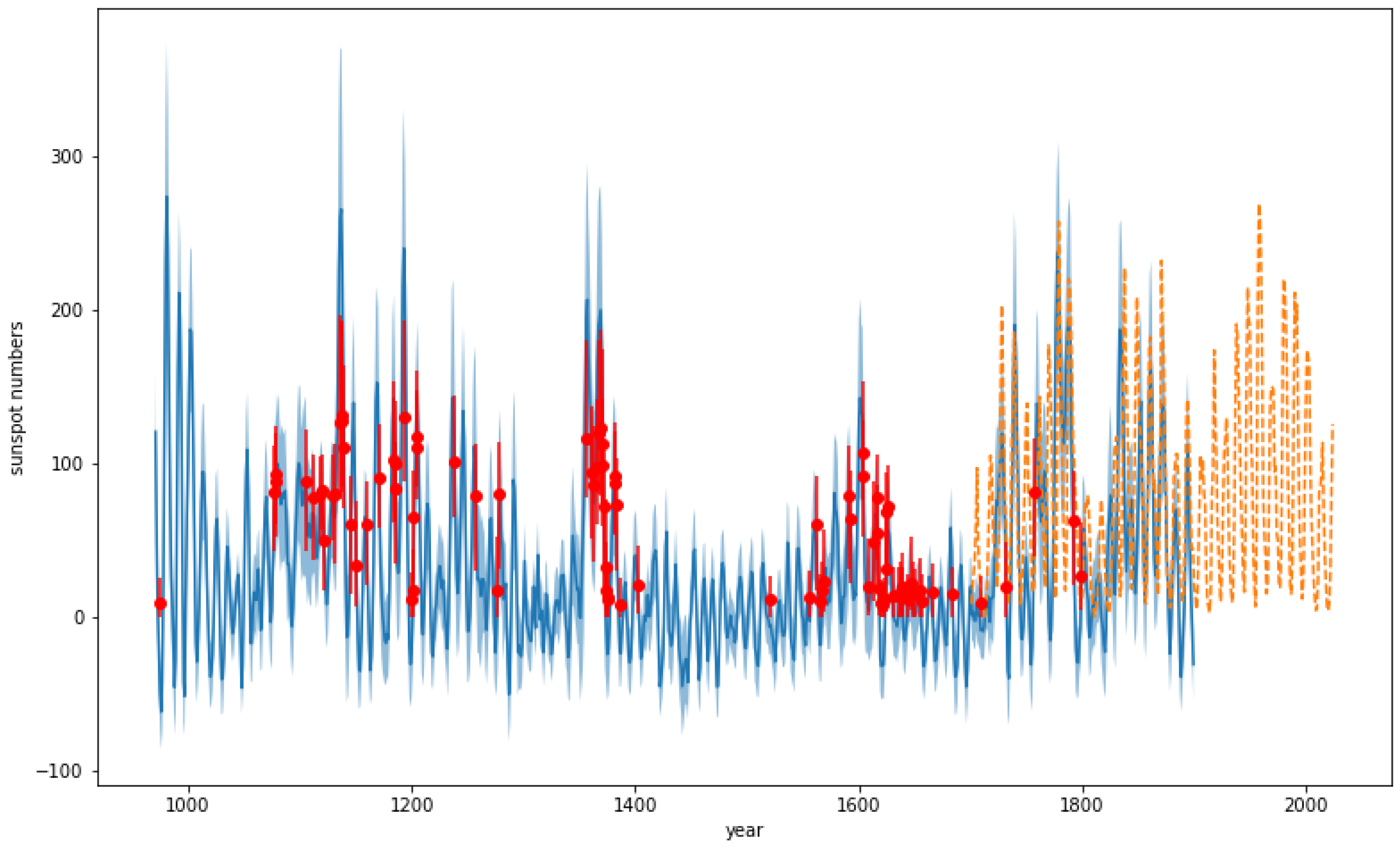
3.1. Using NES Information

Using the year 1566 as an example, when there exists a NES record that year, the ¹⁴C reconstruction of the SSN provides a 68% interval $[a,b]=[-41.8,5.0]$. (The year 1566 is chosen only for illustration; there are many other years with NES records and ¹⁴C reconstructions, which could have been used instead.) We use BKI to combine these two pieces of information.

The telescopically observed SSNs with known standard errors for the 22 years between 1818 and 1918, when NES records exist, are used in a prior distribution to update the $68\%$ interval obtained from the ¹⁴C method, $[a,b]=[-41.8,5.0]$, to a Bayesian $68\%$ interval, $[a,b]=[0.0,28.1]$, according to the posterior distribution. There was a reduction in the width of the interval. However, if the ¹⁴C-based interval is zero-truncated to $[a,b]=[0,5.0]$, then combining the telescopic SSN data from NES records actually increases the uncertainty for this particular year. If all the telescopically observed SSNs between 1818 and 2023 are used in the prior distribution, whether or not NES records exists, then the Bayesian posterior $68\%$ interval actually narrows down slightly, to $[a,b]=[1.6,22.4]$. These imply that NES records provide little additional information. This is consistent with the findings of [6], who show that the distributions of GSN do not differ much between years with or without NES records.

When this is repeated on all the 89 years before 1818 when there is both a ¹⁴C reconstruction and an NES record (see Figure 1), we found that the average width of the 68% intervals is $\{83.6,72.0,63.2,61.6\}$, respectively, for the ¹⁴C method, the ¹⁴C method with zero-truncation, the Bayesian method using all post-1818 years’ telescopic SSN information, and the Bayesian method using post-1818 telescopic SSN information from only the NES years. There are some small improvements (about 12%) in reducing the uncertainty caused by using the Bayesian methods; however, after using the SSN information from the telescope observations, adding that the year has an NES causes very little further reduction (less than 3%). All these confirm that NES records provide little additional information in estimation of annual SSN, after using the Bayesian method. The combination of using the Bayesian method AND the NES does lead to a moderate decrease in average interval width (about 15%), compared to the ¹⁴C method with 0-truncation. This leads us to use cross-validation to check if these slightly narrower intervals cover the observed SSNs less often.

Cross-Validation of the Bayesian Results Using NES Information

The observed SSN (with or without knowing its standard error) is known since 1700. There are 27 NES years since then. We use the later 13 NES years (after 1862) to drive the prior distribution used in the Bayesian method, which incorporates the knowledge that these are NES years. The Bayesian estimates using NES information in later years are then tested on the observed SSNs in the earlier 14 NES years (before 1862). We found that the root mean square error between the Bayesian point estimates (the medians) and the observed SSNs is 50.2, which is only slightly less (less than 8%) than the root mean square error between the 0-truncated ¹⁴C estimates and the observed SSNs, which is 54.4. The difference is not statistically significant since out of these 14 NES years, for exactly 7 times the observed SSNs are closer to the Bayesian estimates than to the 0-truncated ¹⁴C estimates.

We found that the average interval widths (for the earlier 14 NES years) for the Bayesian method with NES information is 64.4, compared to 75.3 for average interval width for the 0-truncated ¹⁴C method. This represents about 14% reduction. The narrower intervals did not reduce the empirical coverage. The Bayesian intervals cover the observed SSN 11/14 times compared to 10/14 times for the empirical coverage of the 0-truncated ¹⁴C intervals. However, the reduction of the interval width is not statistically significant, since for 7 times out of these 14 NES years, the Bayesian intervals are wider than the 0-truncated ¹⁴C intervals.

In summary, there is some indication that NES information plus the use of the Bayes method may lead to moderately narrower interval estimates compared to the ¹⁴C method with 0-truncation, without hurting the ability to cover the underlying SSN, but we did not find the supporting evidence to be statistically significant.

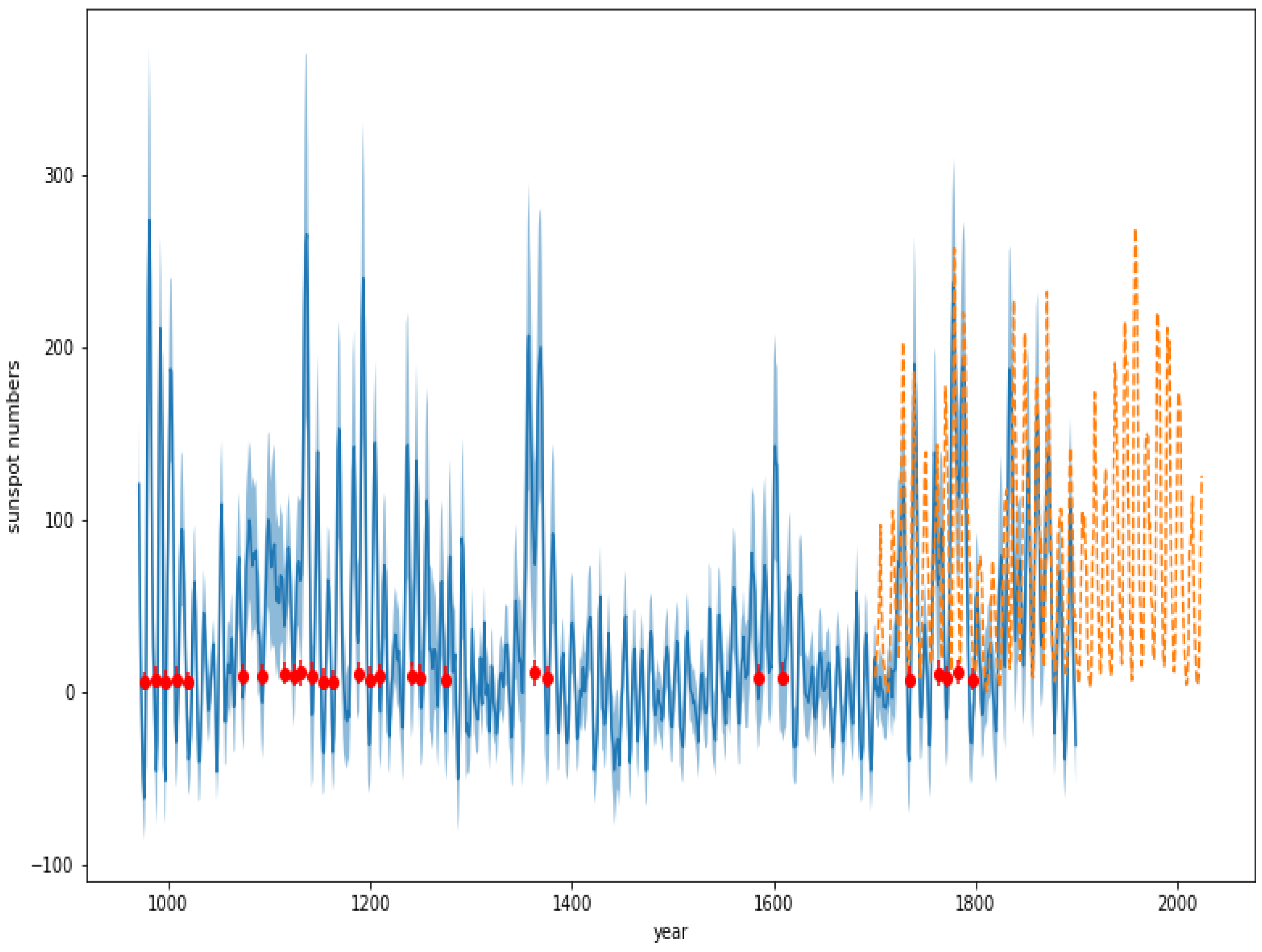
3.2. Using Cycle Minimum Information

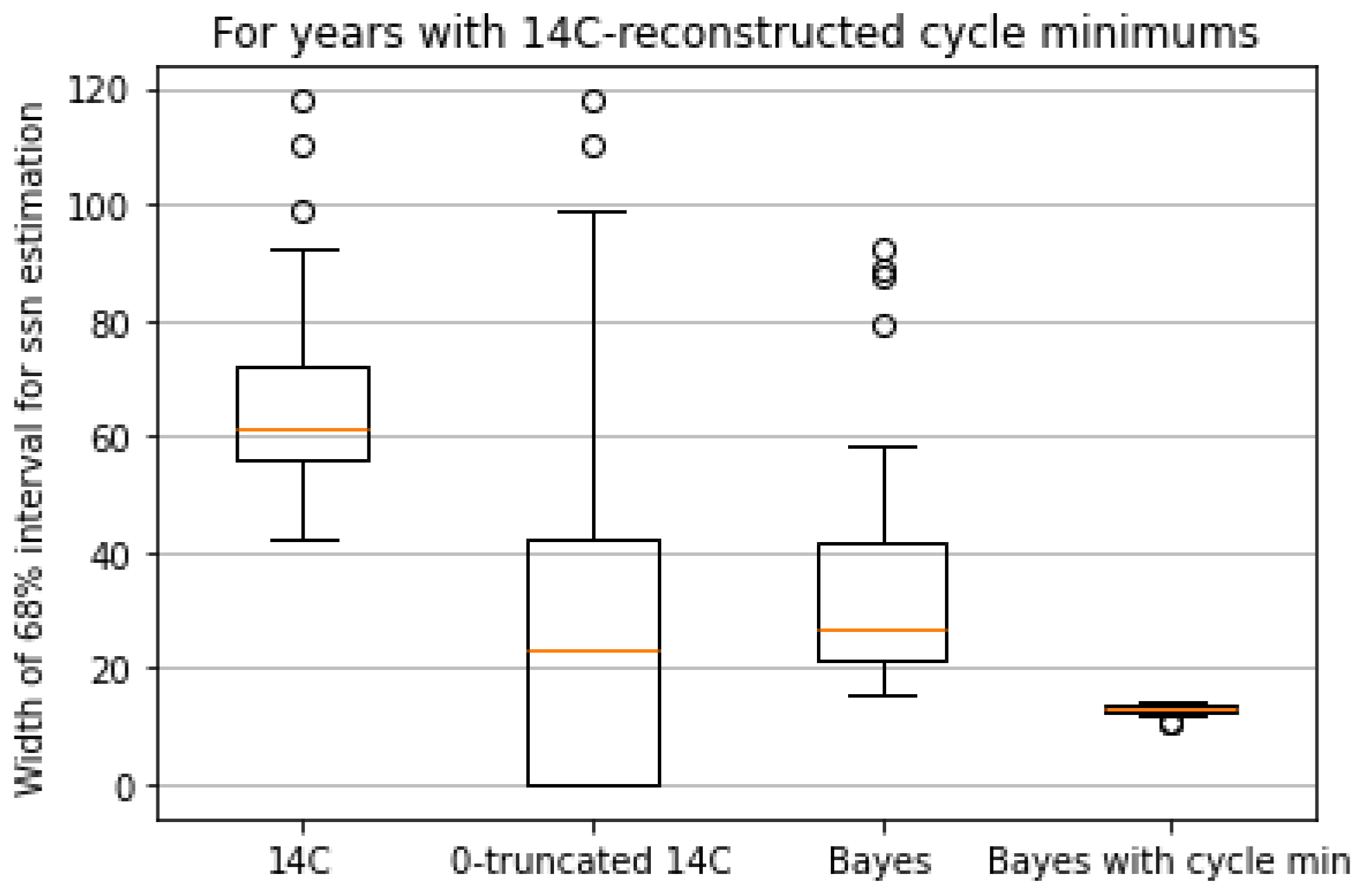
3.2.1. Narrowing of 68% Intervals

There are many approximately 11-year cycles of annual SSN since about 1000 years ago, identified by Usoskin and Solanki et al. (2021) using the ¹⁴C reconstruction method. The locations of cycle maximums and minimums are only approximate, but are found to be typically within $\pm 2$ years comparing to recent telescopic SSN data. We are interested in whether the information of a cycle minimum can help reduce the large amount of uncertainty in the reconstructed SSN. For example, the year 1363 is a cycle minimum, with $74\pm 58.9$ SSN, that is bracketed by two high peaks, one at year 1369 [with SSN in $199.9\pm 80.5$], and one at year 1357 [with SSN in $206.5\pm 89.3$], which are 12 years apart. The actual cycle minimum may not be exactly located at 1363, but we would like to improve the estimation of SNN at this cycle minimum around 1363, regardless of in which year exactly it is located6.

The BKI method combines information from the wide ¹⁴C interval $74\pm 58.9$ with the telescopically observed SSN information from 19 cycle minimums between 1818 and 2023, using their standard errors. The resulting 16%, 50%, and 84% quantiles of the posterior distribution for the SSN are found to be $[a,c,b]=[3.6,11.0,18.1]$, respectively. Therefore, the Bayesian interval has a width $b-a=18.1-3.6=14.5.$ In contrast, the ¹⁴C method gives an interval width of (74 + 58.9) − (74 − 58.9) = 117.8. We see that the Bayesian interval becomes much narrower (about 1:8) in comparison.

In order to assess whether the information of cycle minimum is influential to the Bayesian method, we incorporated the telescopic information on SSNs for all years without restricting to cycle minimums using their standard errors. This time the Bayesian posterior 0.16, 0.50, and 0.84 quantiles become $[a,c,b]=[16.7,60.0,109.2]$, whose range is no longer so much narrower than the ¹⁴C interval (about 4:5 in comparison this time). This shows that information about cycle minimum was highly influential in reducing the uncertainty, in contrast to the information of NES records in the previous analysis.

Side-to-side boxplots in Figure 2 confirm that the same phenomenon appears over all the cycle minimum years from the ¹⁴C reconstruction before 1818. In addition, the average widths for the 68% intervals are 66.8 for the ¹⁴C interval, 30.9 for the 0-truncated ¹⁴C interval, 36.5 for the Bayesian interval using telescopic SSN information from all years after 1818, and 12.9 for the Bayesian interval using telescopic SSN information after 1818 only at the cycle minima. Therefore, the cycle minimum information is very useful in reducing the uncertainty in ¹⁴C reconstruction of the SSN and reduces the average 68% interval width to less than a half. The usefulness of the cycle minimum information is related to the fact that the SSNs in the cycle minimum years are much smaller than the SSNs in other years, which influence the posterior distribution to focus on small and positive SSN values that allow much less uncertainty. In contrast, in the previous exercise, the SSNs in the years with NES records were not so much different from the SSNs in other years, as found in Usoskin et al. (2015) [6]. That is why the NES information was not so useful.

The results of the Bayesian reconstruction for SSN combining ¹⁴C information and cycle minimum information are listed in comparison with the ¹⁴C results in

Table 1. Table of 16%, 50%, and 84% quantiles of SSNs at years of plausible cycle minimums from ¹⁴C reconstruction (last three columns) and from the Bayesian method incorporating the cycle minimum information from later telescope observations (the 2nd to the 4th columns).

Year	$\mathit{Q}\left(0.16\right)$B	$\mathit{Q}\left(0.50\right)$B	$\mathit{Q}\left(0.84\right)$B	$\mathit{Q}{\left(0.16\right)}^{14}$C	$\mathit{Q}{\left(0.50\right)}^{14}$C	$\mathit{Q}{\left(0.84\right)}^{14}$C
1796	1.36	6.18	13.45	−51.5	−29.9	−8.3
1783	4.48	11.8	18.48	63.4	112.7	162.0
1771	2.41	7.86	15.41	−43.9	−15.5	12.9
1763	3.53	10.04	17.84	6.7	61.7	116.7
1734	2.11	7.11	15.05	−70.8	−40.1	−9.4
1609	3.08	8.42	17.29	−29.0	4.0	37.0
1584	2.85	8.43	16.33	−33.7	−4.3	25.1
1375	2.41	7.75	15.43	−54.6	−24.5	5.6
1363	3.56	10.97	18.06	15.1	74.0	132.9
1275	2.26	7.0	14.61	−51.7	−23.5	4.7
1250	2.79	8.45	15.86	−42.7	−9.5	23.7
1241	3.47	9.62	17.4	−27.0	15.2	57.4
1210	2.57	8.48	16.18	−45.6	−11.6	22.4
1199	2.05	7.0	14.66	−59.1	−30.9	−2.7
1188	4.13	9.85	17.1	−16.2	28.5	73.2
1163	0.92	5.25	12.67	−57.5	−35.0	−12.5
1154	1.09	6.0	13.26	−58.5	−35.4	−12.3
1142	3.03	8.51	16.78	−55.8	−13.4	29.0
1131	3.62	11.08	17.86	18.3	64.6	110.9
1124	3.17	8.81	16.57	−20.8	8.0	36.8
1115	4.1	10.62	17.63	5.2	38.0	70.8
1093	2.8	8.59	16.16	−39.0	−6.3	26.4
1074	3.29	8.86	15.98	−34.5	−3.6	27.3
1020	1.09	5.49	11.78	−60.1	−39.1	−18.1
1008	1.8	6.81	14.85	−56.2	−29.4	−2.6
997	1.6	5.5	12.43	−77.3	−51.8	−26.3
988	1.89	6.51	14.53	−77.1	−46.0	−14.9
976	1.07	5.4	11.5	−86.4	−62.0	−37.6

.

In Figure 3, the Bayesian point estimates and 68% intervals for SSNs at plausible cycle minimums are plotted over the years and compared to the ¹⁴C reconstruction and to the telescopically observed SSNs in the later years.

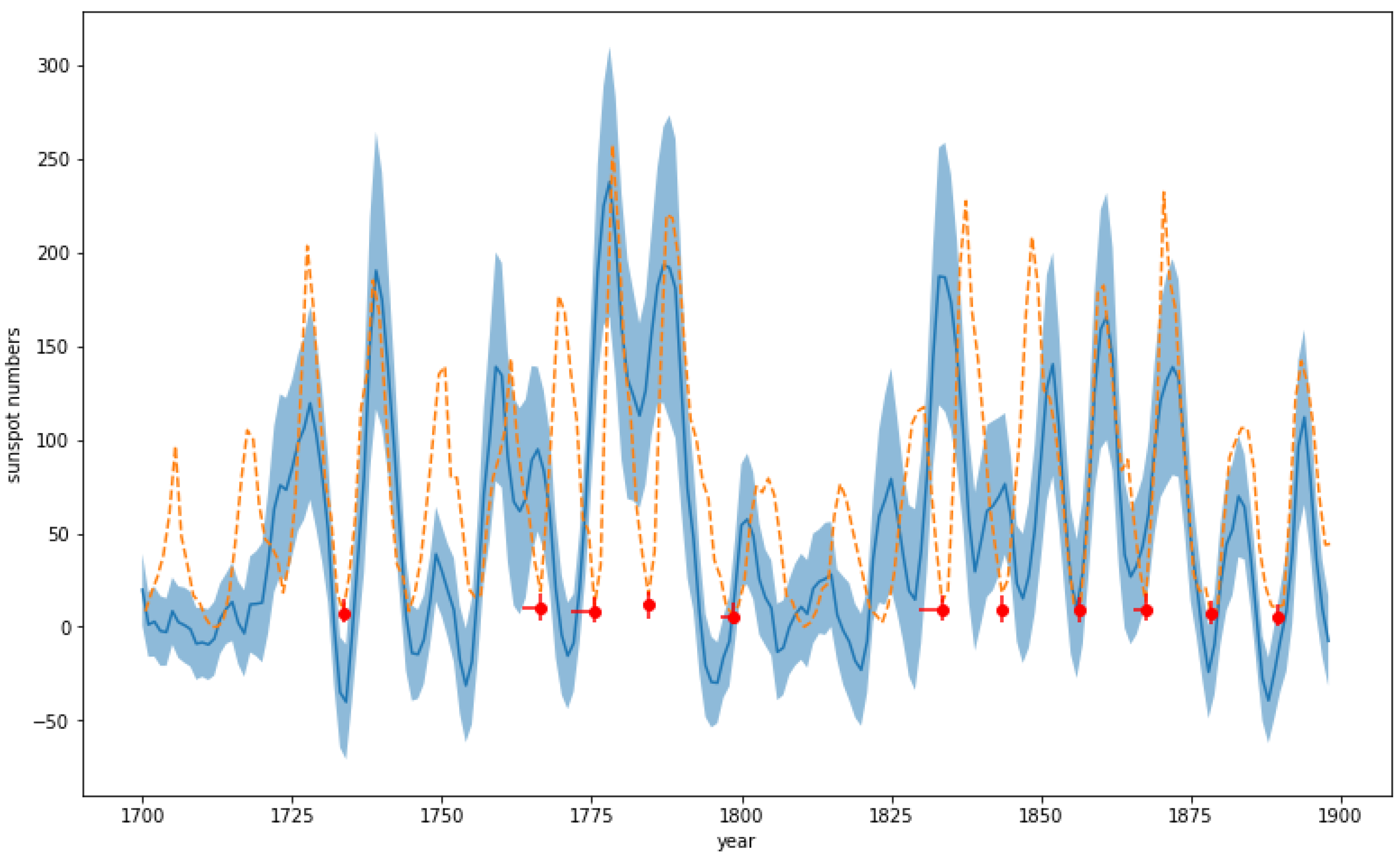
3.2.2. Cross-Validation of the Bayesian Results Using Cycle Minima Information

An important question is: will the much narrowed Bayesian intervals miss the observed SSN by a bigger amount, or miss more often?

To test whether the observed SSN in a year is missed by the Bayesian interval, we would like to use the idea of cross-validation and to make sure that this observed SSN to be tested is not used in the prior distribution when computing the Bayesian interval. We use cycle minimum years before 1899 to test if their SSNs are missed since after 1899, the ¹⁴C reconstruction data are not available for use in the Bayesian method. This implies that we should only use the data after 1899 to construct the prior distribution for computing the Bayes intervals.

For the SSNs to be tested, we select 11 cycle minimum years for the observed SSNs between 1700 and 1899. For each of these 11 years, a nearest minimum according to the ¹⁴C reconstruction is found to be a plausible cycle minimum in the sense of note 3. The SSN cycle-minimum year 1843 is special, since two ¹⁴C-plausible-cycle-minimum years are its equally distant nearest neighbors, each being 4 years apart. We take the average for these two nearest neighbor cycle minimums according to the ¹⁴C reconstructions.

For the Bayes method, we use the non-overlapping telescopic SSN data from the 12 cycle minimums after 1899 to derive the posterior distribution for each of the 11 cycle minimums before 1899 and compute its 0.16, 0.50, and 0.84 quantiles. The 0.16, 0.50, and 0.84 quantiles are also obtained for the ¹⁴C reconstruction method. The details of these quantiles can be seen in

Table 2. Table of observed cycle minimum SSN (the 5th column) and its year (the 6th column), 16%, 50%, and 84% quantiles of SSN at years of plausible cycle minimums from ¹⁴C reconstruction (last three columns), and from the Bayesian method using the cycle minimum information (the 2nd to the 4th columns). The first column is the year of the nearest-neighbor plausible cycle minimum(s) (defined according to note 3, with ties being averaged), as identified by the ¹⁴C method. These 11 cycle minimums are taken from between 1700 and 1899, when both telescope observations of SNN and the ¹⁴C reconstructions in [2] are available. The values from the Bayesian method have some minor differences from those on Table 1, since here only non-overlapping cycle minimums after 1899 are incorporated in the prior distribution for Bayesian computation.

Yr14C	$\mathit{Q}\left(0.16\right)$B	$\mathit{Q}\left(0.50\right)$B	$\mathit{Q}\left(0.84\right)$B	ObsSSN	YrObs	$\mathit{Q}\left(0.16\right)$14C	$\mathit{Q}\left(0.50\right)$14C	$\mathit{Q}\left(0.84\right)$14C
1888	0.7	5.33	12.41	10.4	1889	−62.1	−39.3	−16.5
1878	1.87	6.75	14.2	5.7	1878	−48.9	−24.1	0.7
1865	3.21	9.48	17.47	13.9	1867	−9.3	26.8	62.9
1856	2.64	8.66	16.29	8.2	1856	−27.4	9.6	46.6
1847, 1839	2.65	8.75	17.27	18.1	1843	−16.1	22.3	60.7
1829	3.15	9.09	17.05	13.4	1833	−33.8	14.5	62.8
1796	1.47	5.66	12.77	6.8	1798	−51.5	−29.9	−8.3
1783	4.14	11.68	18.63	17.0	1784	63.4	112.7	162.0
1771	2.23	7.7	15.92	11.7	1775	−43.9	−15.5	12.9
1763	3.17	10.08	18.1	19.0	1766	6.7	61.7	116.7
1734	2.03	7.29	14.48	8.3	1733	−70.8	−40.1	−9.4

, where the actual telescopic SSN data are also listed for comparison.

In Figure 4, the Bayesian point estimate and 68% intervals for the SSNs at these 11 cycle minimums are plotted over the years before 1899 and compared to the ¹⁴C reconstruction and to the unused information on telescopic SSNs. We can see that the Bayesian reconstruction tends to have fewer uncertainties and tends to be closer to the telescopic SSNs.

When we obtain the ¹⁴C-based point estimates and 68% intervals, we assume that the uncertainty related to ¹⁴C reconstruction is normally distributed, which is alluded to in the discussion of Section 3.4 in [2]. The intervals of the Bayesian method are obtained non-parametrically and may not be symmetric. Now we check the “empirical coverage” of the 68% intervals and the root mean square errors of the corresponding point estimates based on Section 2. For each year $j=1,\dots ,11$ of this set of 11 years, we compute the point estimate and the 68% interval for the Bayesian method and the ¹⁴C method with and without 0-truncated, respectively. The 68% intervals based on ¹⁴C reconstruction cover the observed SSN 6/11 ≈ 54.5% times, with an average interval width of $71.3$ or 41.4 after applying 0-truncation. The 68% intervals from the Bayesian method using the cycle minimum information cover the observed SSN 9/11 ≈ 81.8% times, despite having a much narrower mean interval width of only about $13.4$. The empirical coverage 81.8% is higher than the nominal coverage 68%. This is not surprising, since the empirical coverage, even for a perfect 68% interval over only 11 trials, has a large standard deviation of $\sqrt{0.68\ast (1-0.68)/11}\approx 14\%$. The higher than-nominal empirical coverage may also be caused by our computation method in Section 2 using some conservation approximations.

If we compare the point estimates to the observed SSNs for these 11 years, the point estimate $max\{Y_j,0\}$’s based on the 0-truncated ¹⁴C reconstruction achieves a root mean square error of 32.4, while the Bayesian estimate (the posterior median $Q_j\left(0.50\right)$) achieves a root mean square error of about 5.0, only about 1:6 as large.

The absolute differences of these point estimates from the observed SSN $R_j$’s are compared by taking pairwise differences:

$$|Q_j\left(0.50\right)-R_j|-|max(0,Y_j)-R_j|,j=1,\dots ,11.$$

Only 2/11 of such differences are positive. The chance of observing 2 or less such positive differences randomly out of 11 trials is the probability of a Binomial(11, 0.5) random variable being 0, 1, 2, which is only (1 + 11 + 11 * 10/(2 * 1))/2¹¹, about 0.033. We have relatively strong statistical evidence that the Bayesian estimates are closer to the telescopically-observed SSN values, compared to the zero-truncated ¹⁴C estimates.

4. Conclusions

We apply a Bayesian method to infuse additional information into a “target” measurement result, here being the estimated SSN from the ¹⁴C reconstruction. An example of additional information that is not very effective for improving the ¹⁴C reconstruction is that a certain year is included in the Far Eastern NES catalog. In contrast, an example of very effective additional information for improving the ¹⁴C reconstruction is that a certain year is a cycle minimum. This method may be adapted to other applications for reducing uncertainty with effective additional information.

The BKI method requires choosing a prior distribution properly. In our application, it involves the decision about which years with telescopically observed SSNs are regarded as “similar years” that are similar to a “target year”. The pre-conditions themselves are easy to check, e.g., which of the years in the telescopic era have NES records, or which years are cycle minimums. When the target year satisfies a pre-condition, we can select similar years in the telescopic era that satisfy the same pre-condition. However, any subset of these years could be used, and when we change the subset of “similar years” used in the prior distribution for BKI, the results will differ. For example, the target year 1796 is a cycle minimum according to the ¹⁴C reconstruction, and it appears both in Table 1 and Table 2. The prior distribution used for Table 1 uses all 19 telescopically observed cycle minimums between 1818 and 2023. The prior distribution for Table 2 only uses 12 telescopically observed cycle minimums after 1899. This causes the resulting (0.16, 0.50, 0.84) quantiles of the posterior distributions to change from (1.36, 6.18, 13.45) to (1.47, 5.66, 12.77). Although the change is minor in this case, one can imagine that bigger changes could happen when a different subset of years is used in the prior distribution.

The following are some recommendations:

• When we are not sure, we propose to use all years available that satisfy the pre-condition to account for the uncertainty in our knowledge as much as possible. This is the approach we take in the current paper.
• It may be safer to report a result together with the corresponding assumption, e.g., “Assuming that the target year 1796 is similar to the cycle minimum years after 1899, then the posterior quantiles for the SSN in year 1796 will be (1.47, 5.66, 12.77)”.
• Subject matter knowledge may help to tell if a subset of years are similar to the target year, or none of the years in the telescopic era is similar to the target year, and a scaling up or long-term de-trending (say) of the SSN values has to be done first before applying BKI. (So we may regard BKI as a mathematical framework that can be made useful with additional scientific knowledge).

References

1. Solanki, S.K.; Usoskin, I.G.; Kromer, B.; Schüssler, M.; Beer, J. Unusual activity of the Sun during recent decades compared to the previous 11,000 years. Nature 2004, 431, 1084–1087. [Google Scholar] [CrossRef] [PubMed]
2. Usoskin, I.G.; Solanki, S.K.; Krivova, N.A.; Hofer, B.; Kovaltsov, G.A.; Wacker, L.; Brehm, N.; Kromer, B. Solar cyclic activity over the last millennium reconstructed from annual 14C data. Astron. Astrophys. 2021, 649, A141. [Google Scholar] [CrossRef]
3. 1000-Year Sunspot Series (Usoskin+, 2021). Available online: http://cdsarc.u-strasbg.fr/ftp/J/A+A/649/A141/ (accessed on 11 September 2024).
4. Brehm, N.; Bayliss, A.; Christl, M.; Synal, H.A.; Adolphi, F.; Beer, J.; Kromer, B.; Muscheler, R.; Solanki, S.K.; Usoskin, I.; et al. Eleven-year solar cycles over the last millennium revealed by radiocarbon in tree rings. Nat. Geosci. 2021, 14, 10–15. [Google Scholar] [CrossRef]
5. Yau, K.K.C.; Stephenson, F.R. A revised catalogue of Far Eastern observations of sunspots (165 BC to AD 1918). Q. J. R. Astron. Soc. 1988, 29, 175–197. [Google Scholar]
6. Usoskin, I.G.; Arlt, R.; Asvestari, E.; Hawkins, E.; Käpylä, M.; Kovaltsov, G.A.; Krivova, N.; Lockwood, M.; Mursula, K.; O’Reilly, J.; et al. The Maunder minimum (1645–1715) was indeed a grand minimum: A reassessment of multiple datasets. Astron. Astrophys. 2015, 581, A95. [Google Scholar] [CrossRef]
7. Hathaway, D.H.; Wilson, R.M.; Reichmann, E.J. The shape of the sunspot cycle. Sol. Phys. 1994, 151, 177–190. [Google Scholar] [CrossRef]
8. Wilson, R.M.; Hathaway, D.H.; Reichmann, E.J. On the importance of cycle minimum in sunspot cycle prediction. NASA Tech. Publ. TP-3648 1996, 16, 1–11. [Google Scholar]
9. Sunspot Data (WDC-SILSO, Royal Observatory of Belgium, Brussels). Available online: https://www.sidc.be/SILSO/DATA/SN_y_tot_V2.0.txt (accessed on 11 September 2024).
10. Minima and Maxima of Sunspot Number Cycles (NOAA). Available online: https://www.ngdc.noaa.gov/stp/space-weather/solar-data/solar-indices/sunspot-numbers/cycle-data/table_cycle-dates_maximum-minimum.txt (accessed on 11 September 2024).
11. Li, Y.R.; Wang, J.M.; Ho, L.C.; Du, P.; Bai, J.M. A Bayesian approach to estimate the size and structure of the broad-line region in active galactic nuclei using reverberation mapping data. Astrophys. J. 2013, 779, 110. [Google Scholar] [CrossRef]
12. Fan, X.; Messenger, C.; Heng, I.S. A Bayesian approach to multi-messenger astronomy: Identification of gravitational-wave host galaxies. Astrophys. J. 2014, 795, 43. [Google Scholar] [CrossRef]
13. Shao, Z.; Xie, X.; Chen, L.; Zhong, J.; Hou, J.; Lin, C.C. Bayesian Inference of Kinematics and Mass Segregation of Open Cluster. Int. Astron. Union. Proc. Int. Astron. Union 2015, 12, 265–266. [Google Scholar] [CrossRef]
14. Kang, X.; He, S.Y.; Zhang, Y.X. A novel stellar spectrum denoising method based on deep Bayesian modeling. Res. Astron. Astrophys. 2021, 21, 169. [Google Scholar] [CrossRef]
15. Yu, Y.; van Dyk, D.A.; Kashyap, V.L.; Young, C.A. A Bayesian analysis of the correlations among sunspot cycles. Sol. Phys. 2012, 281, 847–862. [Google Scholar] [CrossRef]
16. Travaglini, G. Bayesian Methods for Reconstructing Sunspot Numbers Before and During the Maunder Minimum. Sol. Phys. 2017, 292, 23. [Google Scholar] [CrossRef]
17. Velasco Herrera, V.M.; Soon, W.; Hoyt, D.V.; Muraközy, J. Group sunspot numbers: A new reconstruction of sunspot activity variations from historical sunspot records using algorithms from machine learning. Sol. Phys. 2022, 297, 8. [Google Scholar] [CrossRef]
18. Hjort, N.L. Bayesian and Empirical Bayesian Bootstrapping. Preprint Series. Statistical Research Report 1991. Available online: https://www.duo.uio.no/bitstream/handle/10852/47760/1/1991-9.pdf (accessed on 11 September 2024).
19. Murphy, K.P. Conjugate Bayesian Analysis of the Gaussian Distribution. Def 2007, 1, 16. Available online: https://www.cs.ubc.ca/~murphyk/Papers/bayesGauss.pdf (accessed on 11 September 2024).
Figure 1. Bayesian point estimates and 68% intervals (symbolized by red dots with vertical error bars) for the SSNs, computed using post-1818 SSNs at years with NES observations, plotted over the years before 1818, and compared to the 14C reconstruction (solid curve with shade for 68% uncertainty) and to the telescopically observed SSNs (dashed curve).
Universe 10 00370 g001
Figure 2. Information of cycle minimums does further reduce uncertainty of SSN estimated from 14C construction. Each boxplot is from 28 widths of the 68% intervals for the 28 years of plausible cycle minima found from the 14C reconstruction (listed in Table 1). For the boxplot above ‘14C’, the interval width for year j is 2 σ j ; for the boxplot above ‘0-truncated 14C’, the interval width for year j is max { Y j + σ j , 0 } max { Y j σ j , 0 } , where Y j is the 14C reconstruction and σ j is the 1-sigma uncertainty. For both the boxplots above ‘Bayes’ and above ‘Bayes with cycle min’, each interval width is computed as the difference of the 84% quantile and the 16% quantile of the posterior distribution. For ‘Bayes with cycle min’, the prior distribution uses the telescopic observations of annual SSNs, only at years of cycle minima, between years 1818 and 2023. For ‘Bayes’, the prior distribution uses all the telescopic observations of annual SSNs, whether or not at cycle minima, between years 1818 and 2023.
Universe 10 00370 g002
Figure 3. Bayesian point estimates and 68% intervals (symbolized by red dots with vertical errorbars) of the SSNs, incorporating telescopic data after 1818, at plausible cycle minimums before 1818, plotted over the years, compared to the 14C reconstruction (solid curve with shade for 68% uncertainty) and to the telescopic SSNs in the later years (dashed curve).
Universe 10 00370 g003
Figure 4. Bayesian reconstruction for SSNs at 11 cycle minimums before 1899, using post-1899 telescopic data at the cycle minimums, plotted over the years, compared to the 14C reconstruction (solid curve with shade for 68% uncertainty) and to the unused information on telescopic SSNs (dashed curve). The red dots and the vertical error bars display the Bayesian point estimate (posterior median) and the nominal 68% intervals. The horizontal error bars extend to the year of the nearest plausible cycle minimum according to the 14C reconstruction, as defined in note 3, with ties averaged. Therefore, the lengths of the horizontal error bars reflect the errors of placements of the cycle minimums by the 14C reconstruction.
Universe 10 00370 g004