Time Scales of Slow-Roll Inflation in Asymptotically Safe Cosmology

Abstract

Making use of the well-known renormalization group (RG) scale dependences of the gravitational couplings in the framework of the two-parameter Einstein–Hilbert (EH) theory of gravity, the single scalar field-driven cosmological inflation is discussed in a spatially homogeneous, isotropic, and flat model universe. The inflaton field is represented by a one-component real, non-self-interacting, massive scalar field minimally coupled to gravity. Cases without and with the incorporation of the RG scaling of the inflaton mass are compared with each other and with the corresponding classical case. It is shown that the quantum improvement drastically alters the timing of the slow-roll inflation with the desirable number $\underset{,}{\mathrm{N}}\approx 60$ e-foldings, as compared with the classical case. Furthermore, accounting for the RG flow of the inflaton mass has an enormous effect on the timing of the desirable slow roll, too. Although providing the desirable slow-roll inflation, none of the versions of the investigated quantum-improved toy models provide a realistic value of the amplitude of the scalar perturbations.

1. Introduction

Asymptotically safe cosmology [1,2,3,4,5,6,7,8,9,10,11,12,13] relies on the success of the asymptotic safety scenario [14] in quantum gravity achieved in the last two decades (see the status reports in [15,16,17] and the references therein). Based on the renormalization group (RG) studies of the four-dimensional two-parameter EH gravity in the continuum, good evidence is found on the existence of an ultraviolet (UV) fixed point, the so-called Reuter fixed point, and that of the Gaussian fixed point [18,19,20,21,22,23,24,25,26,27]. Recently, it has been shown that the particle physics Standard Model coupled to gravity also exhibits asymptotic safety. In general, asymptotic safety sets an upper bound on the number of the various kinds of matter fields, and the suggestion has been put forward that asymptotic safety may serve as a requirement to select physically reliable field theories incorporating the dark constituents of the universe [26,28,29,30,31,32,33,34,35,36].

In this paper, we discuss the possibility of a single real scalar field-driven slow-roll inflation and its characteristic time scales in a quantum-improved toy model of the universe, incorporating the inflaton field $\phi$ and the running cosmological constant $\Lambda$ as the only constituents. The main features of the RG flow of the gravitational couplings in pure gravity are discussed in detail in [37] and appear to be rather independent of the fine details of the RG scheme used. Moreover, the RG analyses of the Euclidean and Lorentzian theories yield rather similar results in that respect [38,39,40,41,42], and the presence of matter is represented only by a single inflaton field does not alter them significantly (see, e.g., Figure 4 in Ref. [26], Figure 6 in Ref. [12], Figure 1 in Ref. [31]). Therefore, we consider the RG flow of the gravitational couplings, that of the Newton coupling $G\left(k\right)$, and the running cosmological constant $\Lambda \left(k\right)$ to be given by the interpolation formulas proposed by us recently in Ref. [43]. It should be pointed out here that the RG flow reflected by our interpolation formulas relies basically on functional RG studies in which the basic object is the effective average action, and the IR regulator contains the four-dimensional Laplacian of spacetime. The identification of the IR cut-off scale k is, however, not unique. Recently, it has been shown that asymptotically safe gravity can be formulated in a consistent manner in the framework of functional RG using the time-slicing corresponding to the ADM decomposition and defining the IR regulator in terms of the spatial Laplacian [38]. As to the asymptotically safe cosmological models, the manner of the identification of the IR cut-off k seems to be crucial from the point of view of whether the initial singularity can be avoided or not. The authors of Ref. [7] have found that bouncing solutions can be found using the functional RG framework proposed in [38], while the universe does not violate the standard energy conditions; even a spatially flat model is strongly favored by the recent observational data. In contrast, in our present work, only solutions with the initial Big Bang singularity can occur for the emerging universe.

Coming back to our interpolation formulas proposed in [43], those reflect the various scaling regimes and the orders of magnitude of their boundaries along the RG energy scale k. The RG flow of the gravitational couplings reveals three scaling regions [37]: the UV regime governed by the Reuter fixed point (FP) for $k\ge k_G\sim \mathcal{O}\left(m_{\mathrm{Pl}}\right)$, the crossover regime for $k_G\ge k\ge k_{\Lambda }\sim \mathcal{O}\left({10}^{-30}{k}_G\right)$ ended in the perturbative one close to the Gaussian FP, and the infrared (IR) region for $k\le k_{\Lambda }$ where the gravitational couplings take their present-day constant values $G_0=m_{\mathrm{Pl}}^{-2}$ (with the Planck mass $m_{\mathrm{Pl}}=\sqrt{\hslash c/G_0}$ in the units $\hslash =c=1$) measured at the laboratory scale $k_l\approx 8.2\times {10}^{-34}{m}_{\mathrm{Pl}}\approx {10}^{-3}{k}_{\Lambda }$ and ${\Lambda }_0\approx 2.7\times {10}^{-122}{m}_{\mathrm{Pl}}^2$ observed at the Hubble scale $k_H\approx 8.2\times {10}^{-62}{m}_{\mathrm{Pl}}\ll k_{\Lambda }$. (It should be noticed that there may exist a deep IR regime for $k\lesssim k_l\sim \mathcal{O}\left({10}^{-3}{k}_{\Lambda }\right)$, where the gravitational couplings G and $\Lambda$ tend to zero in the limit $k\to 0$ [6]; this scaling region can affect, however, the evolution of the universe in the late future, which is out of the scope of our discussion in the present paper.)

It is one of the key tasks in asymptotically safe gravity and cosmology, as well as the physical interpretation of the running of the couplings with the RG scale k. There are good arguments against identifying the k-dependent couplings $G\left(k\right)$ and $\Lambda \left(k\right)$ with the running couplings $G\left(p\right)$ and $\Lambda \left(p\right)$ describing changes in physical amplitudes with the energy scale p of the external momenta due to quantum corrections [44,45,46,47]. In this paper, we restrict ourselves to the cosmology based on the homogeneous and isotropic sector of EH gravity. The effective average action of EH gravity does not incorporate derivative terms with scale-dependent form factors associated with the scalar curvature and the Weyl curvature, i.e., momentum-dependent vertex functions [45,46,47]. Therefore, no dependence on the physical momentum of the Newton coupling can occur explicitly. A more general ansatz for the effective average action, incorporating momentum-dependent vertex functions, would yield, e.g., a graviton propagator depending on the RG scale k as well as on the physical momentum p below the running cut-off k and could provide a change in Newton’s law of gravity with the RG scale k [45,46,47], a “krunning” of “prunning” (with the terminology of [45]). In the framework of EH gravity-based cosmology, however, all couplings, those of gravity and matter, figuring in the effective average action depend only on the RG scale k. Moreover, quantum-improved cosmology, in the manner it is invented here, does not even work with the effective average action explicitly, replacing instead the physically observable coupling constants $G_0$ and ${\Lambda }_0$ by their counterparts in the Friedmann equations directly. If one reconstructs the corresponding effective average action, one could determine the graviton propagator at any scale k in a similar manner illustrated, e.g., in the example of the Green functions of the scalar fields in [48]. The determination of that kind of k-dependent modification of Newton’s law of gravity is, however, out of the scope of the present paper.

For the emergent universe, one naturally expects that the decreasing energy scale k should correspond to increasing cosmological time t, given by some t-to-k conversion rule, $k=k\left(t\right)$. The RG studies prove that the Newton coupling $G\left(k\right)$ vanishes at the Reuter FP, making it plausible that the evolution equations, the quantum-improved Friedmann equations, should keep their classical form with the only modification that Newton’s gravitational constant $G_0$ and the cosmological constant ${\Lambda }_0$ (the null index indicates the present-day values) should be replaced by their time-dependent counterparts $G\left(t\right)\equiv G\left(k\right(t\left)\right)$ and $\Lambda \left(t\right)\equiv \Lambda \left(k\right(t\left)\right)$, respectively. In Ref. [43], we applied the interpolation formulas to a rather simple, analytically solvable model of the universe containing a single barotropic fluid. Here, we apply the interpolation formulas to the model in which matter is represented by a one-component real, massive, but non-self-interacting scalar field $\phi$. Our main goal is to discuss the influence of quantum improvement on slow-roll inflation. Moreover, we intend to reveal separately how the RG flow of the gravitational couplings and that of the inflaton mass affect the existence and the time scales of the slow-roll inflation. Therefore, we investigate here two versions of the quantum-improved toy model (QIM): first neglecting (QIM1) and later taking into account (QIM2) the run of the inflaton mass.

Now, the question arises: do we have an overall picture of the flow of the mass parameter $m^2\left(k\right)$, which might include various scaling regimes from the UV scale to the deep IR regime? Great efforts have been made recently to obtain such a picture of the various couplings of matter in the framework of the particle physics Standard Model (and its possible extensions) coupled to asymptotically safe gravity [9,10,11,12,30,31,34,35,36]. Pure gravity theory seems to exhibit asymptotic safety, i.e., Reuter FP, reflecting the occurrence of quantum scale symmetry in the UV regime: a finite number of dimensionless relevant couplings tend to constant non-vanishing values in the limit $k\to \infty$, while the other couplings are irrelevant. This has the consequence that a UV scaling regime exists [28]. Asymptotic safety may or may not be destroyed by the presence of various numbers of various types of fields. As a rule, quantum gravity effects are produced in the UV regime anti-screening of the Newtonian coupling, while, for example, scalar fields, which we are interested in here, produce a screening effect. For a sufficient number of scalar fields, the screening effect may overcome the anti-screening effect, and asymptotic safety may be destroyed [28].

For our present model, the earlier works are more relevant in which the functional RG analysis has been performed for EH gravity (and its extension, including higher powers of the scalar curvature) coupled to a single scalar field [49,50,51]. The discussion concentrated basically on the existence of the Reuter FP in the framework of the Euclidean theory. In [50], using the de Donder gauge, Litim’s optimized regulator, and the truncated Taylor expansion of the potential and that of the coefficient of the R term in powers of ${\phi }^2$ at ${\phi }^2=0$, it has been established that there exists only a single non-spurious and non-trivial UV FP, the so-called Gaussian Matter FP (GMFP) for the number of dimensions $d=4$ of spacetime. At the GMFP, the gravitational couplings approach the Reuter FP (${\lambda }_{\ast }=0.1814$, $g_{\ast }=0.8375$ in our notations; see Table I in Ref. [50]), while the matter couplings (including mass and self-interaction) tend to zero in the limit $k\to \infty$. Similar results have been obtained in Ref. [12] for the matter content with a single scalar field (c.f. eq. (11) in Ref. [12]). The RG flow equations are explicitly given in a general form (see App. A in Ref. [50]) and are applicable to our model. Solving those for our particular case, we have established that two non-Gaussian UV FPs exist: the one with vanishing dimensionless inflaton mass is a hyperbolic one, and the one with non-vanishing dimensionless inflaton mass is UV attractive and provides asymptotic safety. In Section 4.1, we obtain an overall picture of the global RG flow of the inflaton mass $m\left(k\right)$ covering all scales from the high UV to the IR ones, similar to that expressed by our interpolation Formulas (3) and (4) below for the flow of the gravitational couplings found previously in Ref. [43]. We find that the RG flow of the inflaton mass introduces a new energy scale $k_m>k_G$: the dimensionless inflaton mass is constant for $k>k_m$, the dimensionful inflaton mass takes the constant value at $k\approx k_G$, and $k_m>k>k_G$ is a crossover regime for the RG flow of the inflaton mass. Here, it should be noted that our interpolation Formulas (3) and (4) refer to pure EH gravity without any matter. It has been shown that adding minimally coupled matter fields, either screen (for scalars and fermions) or antiscreen (for gauge fields), the Newton coupling (see [12] and the references therein). Nevertheless, if the numbers of these fields are treated as continuous parameters, the UV FP values and their critical exponents vary continuously in a rather wide range, including the cases with the numbers $N_S=0$ and 1 of the scalar fields. Furthermore, the screening effect is rather small for a single scalar field [12,26,31]. Therefore, we shall use the same interpolation formulas in both cases, QIM1 and QIM2.

So far, the quantum fluctuations of the metric and those of the matter fields are neglected, and the cosmological evolution of the homogeneous and isotropic universe is described by the quantum-modified Friedmann equations and their consistency condition, where the gravitational constants are replaced by their time-dependent counterparts. These equations represent the symmetry-reduced sector of the quantum-improved version of classical EH gravity when the gravitational constants $G_0$ and ${\Lambda }_0$ are replaced by their time-dependent counterparts. Then, the Bianchi identity ${\nabla }_{\mu }{G}^{\mu \nu }=0$ (for the Einstein tensor $G^{\mu \nu }$) implies the quantum-improved consistency condition ${\nabla }_{\mu }\left[G\left(t\right)T^{\mu \nu }\right]=0$ of the Einstein equations with the stress-energy tensor of matter $T^{\mu \nu }$. Having performed the symmetry reduction to the homogeneous and isotropic sector, one obtains the quantum-improved consistency condition (c.f. Equation (10) below) of the quantum-improved Friedmann equations, which is not identical now with the law of the local energy conservation of matter, as it was in the classical case. In the discussed model, the cosmological evolution of the homogeneous background can be formulated in terms of the Hubble parameter $H\left(t\right)$, the scalar field $\phi \left(t\right)$, and the function $k\left(t\right)$. Then, one has only two independent equations for the determination of 3 yet unknown functions. Regarding this problem, various approaches have been worked out in the literature. The first attempts assumed that one has to make some intuitive assumption on the function $k\left(t\right)$, like $k=\xi /t$ with some constant $\xi$, require the local conservation of the energy of matter separately, like in classical cosmology [52], and adjust the constant $\xi$ in the UV and in the perturbative regimes separately in order to achieve consistency among the four equations [53,54]. These first efforts have made a hint on the scale- or time-dependence of $\xi$ itself: different results have been obtained for $\xi$ in the UV and in the perturbative regimes. Here, we apply the approach rather close to that proposed in Ref. [55] that determines the function $k\left(t\right)$ from the interplay between the Klein–Gordon (KG) equation of the inflaton field and the quantum-improved consistency condition and results in the reduced consistency condition (c.f. Equations (11) and (13) below). This method reproduces the approach of the authors of Ref. [55] for QIM1 and enables one to account for the running inflaton mass for QIM2. Another approach has been proposed in Ref. [1]: the authors discussed the cosmological system in the framework of the dynamical system analysis in terms of the dimensionless cosmological variables [56,57] when the first Friedmann equation turns out to be rather a constraint and not a dynamical equation, and its differentiation with respect to the RG scale k yields an additional constraint. In Sect. Section 2 we show that this RG-induced constraint is identical to the reduced consistency condition, independently of whether QIM1 or QIM2 is considered. Therefore, our approach to determining the t-to-k conversion rule is identical to the one proposed in Ref. [1].

In our toy model, we identify the presence of the running cosmological constant $\Lambda \left(k\right)$ with that of the dark energy and call the quantity

$$\begin{array}{ccc}\hfill {\rho }^{(\Lambda )}& =& {\displaystyle \frac{\Lambda }{8\pi G}}\hfill \end{array}$$

(1)

the density of the dark energy. It is rather giving a name to the constituent $\Lambda$ of the model; to go beyond the nature of the dark energy is out of the scope of the present paper. Motivated by the interpretation used in [1], we take the point of view that ${\rho }^{(\Lambda )}$ can be considered as the field-independent potential energy density of a condensed scalar field, which implies the EoS $p^{(\Lambda )}=-{\rho }^{(\Lambda )}$ implicitly with the pressure $p^{(\Lambda )}$ of the dark energy. Discussing the description of the evolution of the model universe in terms of the dimensionless variables, the definitions of the latter are chosen in a manner that treats the potential energy density of the scalar field $V_k\left(\phi \right)$ as the sum $V_k\left(\phi \right)={\rho }^{(\Lambda )}\left(k\right)+U_k\left(\phi \right)$, where $U_k\left(\phi \right)\ge 0$ is the field-dependent piece having $U_k\left({\phi }_{\mathrm{m}}\right)=0$ at the local minimum of $U_k\left(\phi \right)$ at $\phi ={\phi }_{\mathrm{m}}$, in general. In our model, $U_k\left(\phi \right)$ represents the simple, generally scale-dependent mass term $U_k\left(\phi \right)=m^2\left(k\right){\phi }^2/2$ and ${\phi }_{\mathrm{m}}=0$.

Below, we shall discuss the evolution of the model universe up to the end of the slow-roll inflationary era. The only free parameter involved in our discussions is the IR value of the dimensionful inflaton mass; the latter is kept constant at all scales in QIM1, while QIM2 involves the running inflaton mass approximated by the interpolation Formula (56) established in Section 4.1. We shall show that in both QIM1 and QIM2, the slow-roll inflation occurs along a universal attractor in the phase space of the scalar field for properly chosen IR values of the inflaton mass, quite similarly as in the classical case [58]. Moreover, we shall argue that the universal attractor is negligibly affected by quantum effects, which die out essentially at the onset of the slow roll. Here, we consider general relativity as well as the quantum-improved theory of EH gravity coupled minimally to the scalar field, not like effective theories, but extrapolate their validity back to the Big Bang. In the classical model (GRM) based on Einstein’s general relativity minimally coupled to the massive, self-interacting scalar field, there occurs an inflationary era characterized by an ultrahard EoS of the scalar field followed by the slow-roll inflationary era itself [58]. In contrast, in QIM1 and QIM2, the evolution scenario appears to be more structured:

• The Big Bang singularity is followed by the Reuter FP-driven era (RFPE). This covers the Planck era ending at $t=t_G\sim \mathcal{O}\left(1\right)$ $s_{\mathrm{Pl}}$ for QIM1, while it ends at $t=t_m\sim \mathcal{O}\left({10}^{-1}\right)$ $s_{\mathrm{Pl}}$ for QIM2. (Here ${\mathrm{s}}_{\mathrm{Pl}}=\sqrt{\hslash G_0/c^5}$ stands for the Planck second, $1{\mathrm{s}}_{\mathrm{Pl}}=1m_{\mathrm{Pl}}^{-1}$ in the units $\hslash =c=1$).
• For QIM2, there occurs the crossover era (COE1) lasting from $t=t_m$ to $t=t_G$, during which the dimensionless gravitational couplings keep their FP values, but the dimensionless inflaton mass changes from its constant FP value to its $\sim 1/k^2$ IR behavior. The duration of COE1 is rather short, so it ends at $t_G\sim \mathcal{O}\left({10}^{-1}\right)$ ${\mathrm{s}}_{\mathrm{Pl}}$.
• The crossover era (COE2) with constant dimensionful inflaton mass, but the crossover scaling behaviors of the gravitational couplings show up in both QIM1 and QIM2 and are followed numerically from $t=t_G$ to the end of the slow-roll inflation at $t=t_f\ll t_{\Lambda }$ settled by the value $\epsilon =1$ of the slow-roll parameter. COE2 starts with a preinflationary era followed by the era of slow-roll inflation, which sets on at $t=t_i\gg t_G$. As it is shown below, during most of the preinflationary era, the kinetic energy density ${\dot{\phi }}^2/2$ of the scalar field dominates over the field-dependent piece $U_k\left(\phi \right)$ of its potential energy density, and the latter takes over when the slow-roll inflation sets on, preceded by the equality ${\dot{\phi }}^2/2=U_k\left(\phi \right)$.
• The discussion of the evolution in terms of the dimensionless quantities [1,56,57] reveals that even the preinflationary era, both in QIM1 and QIM2, is divided into two suberas due to the scale dependence of the dark energy density, i.e., due to quantum effects. Those suberas are separated by the equality of the dark energy density ${\rho }^{(\Lambda )}$ to the potential energy density $U_k\left(\phi \right)$, i.e., ${\rho }^{(\Lambda )}=U_k\left(\phi \right)$.

The times $t_m$ and $t_G$ are defined via the equalities $k\left(t_m\right)=k_m$ and $k\left(t_G\right)=k_G$, respectively, and their orders of magnitude given above belong to the phase trajectories providing the slow-roll inflation, called throughout this paper the desirable one, i.e., the one providing the desirable number $\underset{,}{\mathrm{N}}\approx 60$ of e-foldings. It is the main result of the present paper that the orders of magnitude of the times $t_i$ and $t_f$ are strongly modified by the quantum improvement as compared with the corresponding classical model. Moreover, incorporation of the running inflaton mass may severely influence when the slow-roll inflation sets on.

Following the above-given introduction, we present in Section 2 the toy model of the universe to be discussed. In Section 3, the equations governing the cosmological evolution are specified for QIM1, and the main features of the evolution are discussed in detail in terms of the dimensionful as well as the dimensionless cosmological variables. In Section 4, first, an interpolation formula is derived for the running inflaton mass, exploiting the RG analysis of EH gravity minimally coupled to the scalar field. Then, in Section 4.2, the specification of the equations and the numerically obtained features of the cosmological evolution in QIM2 are presented. Our results are summarized finally in Section 5. In Appendix A, analytic estimates are given for the evolution of RFPE in QIM1. In Appendix B, the quantum-improved universal attractor is discussed, while Appendix C reminds the reader of the features of the universal attractor in GRM. In Appendix D, analytical estimates are given on how the inflaton mass may affect the spectral features of the primordial fluctuations. In Appendix E, analytic estimates are given for the evolution in RFPE in QIM2, while in Appendix F, the elimination of the Hubble parameter from the evolution equations for COE1 is given for QIM2.

2. Model

The classical analog of the system considered here is described by the action

$$\begin{array}{ccc}\hfill S[g_{\mu \nu },\phi ]& =& \mathit{\int }{d}^{4}x\sqrt{-g}\left({\displaystyle \frac{1}{16\pi G_0}}(R-2{\Lambda }_0)-{\displaystyle \frac{1}{2}}{g}^{\mu \nu }{\partial }_{\mu }\phi {\partial }_{\nu }\phi -{\displaystyle \frac{1}{2}}{m}^2{\phi }^2\right),\hfill \end{array}$$

(2)

where $g_{\mu \nu }$ and R are the spacetime metric and scalar curvature, respectively. Matter is represented by the scalar field $\phi$ with the bare mass parameter m. The functional derivative of the action with respect to the metric yields Einstein’s equations, while the functional derivative with respect to the scalar field provides the Klein–Gordon (KG) equation in the curved spacetime. In accordance with the cosmological principle, we consider a model universe that has a spatially homogeneous and isotropic background configuration. Furthermore, we restrict ourselves to the spatially flat case, similar to our present-day universe, according to the observations. Reduction in Einstein’s equations and that of the KG equation to the homogeneous and isotropic sector yields the Friedmann equations and the KG equation for the scalar field in the homogeneous background. So far, no quantum improvement is involved; the KG equation is the consequence of the consistency condition of Einstein’s equations, ${\nabla }_{\mu }(T^{\left(\phi \right)\mu \nu }+T^{(\Lambda )\mu \nu })=0$ reduced to the homogeneous and isotropic sector, where $T^{\left(\phi \right)\mu \nu }$ and $T^{(\Lambda )\mu \nu }$ represent the stress-energy tensor of the scalar field and that associated with the cosmological constant. The quantum improvement of the classical evolution equations is achieved via the replacement of the gravitational couplings $G_0$ and ${\Lambda }_0$ and the bare potential energy density $U\left(\phi \right)$ of the scalar field by their running counterparts $G\left(k\right)$, $\Lambda \left(k\right)$, and $U_k\left(\phi \right)$, respectively. The RG flow of the gravitational couplings is approximated by the formulas given in [43],

$$\begin{array}{ccc}\hfill G\left(k\right)& =& \{\begin{array}{ccc}{g}_{\ast }{k}^{-2}& \mathrm{for}& k_G\le k\\ G_0-b(k^2-k_{\Lambda }^2)=b\left(-k^2+{\displaystyle \frac{1}{2}}E\right)& \mathrm{for}& k_{\Lambda }<k<k_G\\ G_0& \mathrm{for}& 0<k\le k_{\Lambda }\end{array},\hfill \end{array}$$

(3)

$$\begin{array}{ccc}\hfill \Lambda \left(k\right)& =& \{\begin{array}{ccc}{\lambda }_{\ast }{k}^2& \mathrm{for}& k_G\le k\\ {\Lambda }_0+c(k^4-k_{\Lambda }^4)=c(k^4+F)& \mathrm{for}& k_{\Lambda }<k<k_G\\ {\Lambda }_0& \mathrm{for}& 0<k\le k_{\Lambda }\end{array},\hfill \end{array}$$

(4)

where

$$\begin{array}{ccc}& & k_G={\left({\displaystyle \frac{3g_{\ast }}{G_0}}\right)}^{1/2},b={\displaystyle \frac{2G_0^2}{9g_{\ast }}},c={\displaystyle \frac{{\lambda }_{\ast }{G}_0}{3g_{\ast }}},\hfill \end{array}$$

(5)

$$\begin{array}{ccc}& & E=3k_G^2\left(1+{\displaystyle \frac{2}{3}}{\displaystyle \frac{k_{\Lambda }^2}{k_G^2}}\right),F\approx -8.4\times {10}^{-120}{k}_G^4,\hfill \end{array}$$

(6)

and $g_{\ast }\approx 0.71$, ${\lambda }_{\ast }\approx 0.19$, and $k_{\Lambda }=8.2\times {10}^{-31}{m}_{\mathrm{Pl}}$. The interpolation formulas given in [43] contain three free parameters that were determined from the continuity of $G\left(k\right)$, $\Lambda \left(k\right)$, and that of the matter density ${\rho }^{\left(m\right)}$ at the dynamical scale $k_G$, while the scale $k_{\Lambda }\approx 8.2\times {10}^{-31}{m}_{\mathrm{Pl}}$ is taken from the RG analyses [37]. In the space of the dimensionless couplings $(g=G{k}^2,\lambda =\Lambda /k^2)$, the physical RG trajectory relevant to our universe starts at the Reuter FP $(g_{\ast }\approx 0.707,{\lambda }_{\ast }\approx 0.193)$ (The position of the Reuter FP depends slightly on the details of the RG analysis and can be influenced by the matter content of the early universe, but our considerations make use of the existence of the Reuter FP rather than its position); for $k\approx k_{\Lambda }$, it approaches the Gaussian FP at $(g_G=0,{\lambda }_G=0)$, and with the further decrease of the RG scale k, it runs away from the Gaussian FP towards positive values of $\lambda$, while the dimensionful couplings take their present-day observed constant values. The scaling of the couplings slightly above the scale $k_{\Lambda }$ is the so-called perturbative regime. The proposed interpolation formulas recover the UV scaling laws, the constant values $G_0$ and ${\Lambda }_0$ below the scale $k_{\Lambda }$, and in the crossover regime $k\in [k_{\Lambda },k_G]$ are motivated by the scaling in the perturbative regime.

The Friedmann equations read as

$$\begin{array}{ccc}\hfill H^2& =& {\displaystyle \frac{{\kappa }^2}{3}}\left({\rho }^{\left(\phi \right)}+{\rho }^{(\Lambda )}\right),\hfill \end{array}$$

(7)

$$\begin{array}{ccc}\hfill \dot{H}& =& -{\displaystyle \frac{1}{2}}{\kappa }^2{\dot{\phi }}^2\hfill \end{array}$$

(8)

with the energy densities

$$\begin{array}{ccc}\hfill & & {\rho }^{\left(\phi \right)}={\displaystyle \frac{1}{2}}{\dot{\phi }}^2+U_k\left(\phi \right),{\rho }^{(\Lambda )}={\displaystyle \frac{\Lambda \left(k\right)}{8\pi G\left(k\right)}},U_k\left(\phi \right)={\displaystyle \frac{1}{2}}{m}^2\left(k\right){\phi }^2\hfill \end{array}$$

(9)

and ${\kappa }^2=8\pi G\left(k\right)$. The symmetry reduced form of the consistency condition ${\nabla }_{\mu }\left[G(T^{\left(\phi \right)\mu \nu }+T^{(\Lambda )\mu \nu })\right]=0$ of the quantum-improved Einstein’s equations yields the consistency condition

$$\begin{array}{ccc}\hfill {\dot{\rho }}^{\left(\phi \right)}+3H{\dot{\phi }}^2+{\displaystyle \frac{\dot{G}}{G}}{\rho }^{\left(\phi \right)}+{\displaystyle \frac{\dot{\Lambda }}{\Lambda }}{\rho }^{(\Lambda )}& =& 0\hfill \end{array}$$

(10)

of the Friedmann Equations (7) and (8). Here, the dot denotes the total time derivative, i.e., $\dot{f}=(\partial f/\partial t)+(\partial f/\partial lnk)(dlnk/dt)$ for any quantity $f(t;k)$. The KG equation with the scale-dependent potential energy density $U_k\left(\phi \right)$,

$$\begin{array}{ccc}\hfill \ddot{\phi }+3H\dot{\phi }+U_{k,\phi }& =& 0\hfill \end{array}$$

(11)

is equivalent with the continuity equation for the energy density of the scalar field

$$\begin{array}{ccc}\hfill {\dot{\rho }}^{\left(\phi \right)}+3H{\dot{\phi }}^2& =& U_k\left(\phi \right){\nu }_{\mathrm{RG}}{\displaystyle \frac{dlnk}{dt}}.\hfill \end{array}$$

(12)

Equations (12) and (10) provide the reduced consistency condition

$$\begin{array}{ccc}\hfill {\rho }^{\left(\phi \right)}& =& -{\displaystyle \frac{\dot{\Lambda }}{8\pi \dot{G}}}-U_k\left(\phi \right){\displaystyle \frac{{\nu }_{\mathrm{RG}}}{{\eta }_{\mathrm{RG}}}}=-{\rho }^{(\Lambda )}{\displaystyle \frac{{\lambda }_{\mathrm{RG}}}{{\eta }_{\mathrm{RG}}}}-U_k\left(\phi \right){\displaystyle \frac{{\nu }_{\mathrm{RG}}}{{\eta }_{\mathrm{RG}}}}\hfill \end{array}$$

(13)

with the RG parameters

$${\lambda }_{\mathrm{RG}} = {\displaystyle \frac{dln\Lambda }{dlnk}} = \{\begin{array}{ccc}2& \mathrm{for}& k_G\le k\\ {\displaystyle \frac{4k^4}{k^4+F}}& \mathrm{for}& k_{\Lambda }\le k\le k_G\end{array},{\eta }_{\mathrm{RG}} = {\displaystyle \frac{dlnG}{dlnk}} = \{\begin{array}{ccc}-2& \mathrm{for}& k_G\le k\\ {\displaystyle \frac{-2k^2}{-k^2+\frac{1}{2}E}}& \mathrm{for}& k_{\Lambda }\le k\le k_G\end{array},$$

$$\begin{array}{r}{\nu }_{\mathrm{RG}} = {\displaystyle \frac{\partial ln{U}_k\left(\phi \right)}{\partial lnk}} = {\displaystyle \frac{\partial ln{m}^2}{\partial lnk}} \equiv {\beta }_{m^2}.\end{array}$$

(14)

Equation (13) is identical to the RG-induced constraint derived in [1] and reduces to the relation found in [55] when the RG flow of the potential energy density of the scalar field is neglected. Finally, for the determination of the three unknown fields $H\left(t\right)$, $\phi \left(t\right)$, and $k\left(t\right)$, one obtains three independent equations: either the Friedmann Equations (7) and (8) and the RG induced constraint (13) or Equations (7), (11) and (13). To perform the numerical determination of the evolution of the discussed cosmological model, one has to work out the explicit forms of these equations for the Planck and the crossover eras separately. Looking for the presence of the slow-roll inflation and its typical features, we are interested in the evolution only up to the end of the slow-roll inflation at $t=t_f<t_{\Lambda }$.

3. Neglection of the RG Flow of the Inflaton Mass: QIM1

3.1. Evolution in Terms of the Dimensionful Quantities

Making use of the interpolating Formulas (3) and (4), we have to work out the explicit forms of Equations (7), (8) and (13) for QIM1 in RFPE and COE2. In RFPE Equations (7), (8) and (13), they can be recast as

$$\begin{array}{ccc}\hfill 3H^2& =& 8\pi {\rho }^{\left(\phi \right)}{g}_{\ast }{k}^{-2}+{\lambda }_{\ast }{k}^2,\hfill \end{array}$$

(15)

$$\begin{array}{ccc}\hfill \dot{H}& =& -4\pi g_{\ast }{\dot{\phi }}^2{k}^{-2},\hfill \end{array}$$

(16)

$$\begin{array}{ccc}\hfill {\rho }^{\left(\phi \right)}& =& {\displaystyle \frac{{\lambda }_{\ast }}{8\pi g_{\ast }}}{k}^4.\hfill \end{array}$$

(17)

Expressing $k^2$ from Equation (17) and inserting it into Equations (15) and (16), we find a set of coupled first-order ODEs for the functions $H\left(t\right)$ and $\phi \left(t\right)$,

$$\begin{array}{ccc}\hfill 3H^2-2\sqrt{8\pi g_{\ast }{\lambda }_{\ast }{\rho }^{\left(\phi \right)}}& =& 0,\hfill \end{array}$$

(18)

$$\begin{array}{ccc}\hfill 2\dot{H}\sqrt{{\rho }^{\left(\phi \right)}}+\sqrt{8\pi g_{\ast }{\lambda }_{\ast }}{\dot{\phi }}^2& =& 0\hfill \end{array}$$

(19)

with the energy density of the scalar field

$$\begin{array}{c}\hfill {\rho }^{\left(\phi \right)}=({\dot{\phi }}^2+m^2{\phi }^2)/2.\end{array}$$

(20)

Furthermore, due to Equations (15) and (17), the Hubble parameter turns out to be proportional to the RG scale k,

$$\begin{array}{ccc}\hfill H\left(t\right)& =& hk\left(t\right)\mathrm{with}h=\sqrt{{\displaystyle \frac{2{\lambda }_{\ast }}{3}}}.\hfill \end{array}$$

(21)

The condition $k\left(t_G\right)=k_G$ determines the end of RFPE at $t=t_G$. For the initial conditions of the set of Equations (18) and (19), we have chosen the analytically estimated values $H^{\left(\mathrm{est}\right)}\left(t_1\right)$ and ${\phi }^{\left(\mathrm{est}\right)}\left(t_1\right)$ at $t=t_1\ll t_G$ obtained in Appendix A with the approximation that the EoS of the inflaton field is ultrahard just after the Big Bang singularity at $t=0$.

As to the next, let us discuss the evolution of COE2. Making use of the interpolation Formulas (3) and (4), the reduced consistency condition (13) takes the form

$$\begin{array}{ccc}\hfill {\rho }^{\left(\phi \right)}& =& {\displaystyle \frac{c}{4\pi b}}{k}^2.\hfill \end{array}$$

(22)

Instead of solving the system of first-order ODEs (7), (8) and (22) for the three unknown functions $H\left(t\right)$, $k\left(t\right)$, and $\phi \left(t\right)$, it turned out to be more advantageous for the numerics to eliminate the Hubble parameter $H\left(t\right)$ as shown in Appendix B and solve the system of first-order ODEs (A8) and (A9) for the functions $k\left(t\right)$ and $\phi \left(t\right)$ first and evaluate $\dot{\phi }$ from (22) and $H\left(t\right)$ from (7) afterward. The initial conditions for the system of Equations (A8) and (A9) are the values $k\left(t_G\right)=k_G$ and $\phi \left(t_G\right)$ at the end $t=t_G$ of RFPE.

3.2. Numerical Results

Our numerical work has been started by simulating phase trajectories in classical cosmology, i.e., in the framework of GRM. The classical phase trajectories have been generated by solving the KG Equation (A18) given in Appendix C. Throughout our numerical work, we used the observed values $G_0=1m_{\mathrm{Pl}}^{-2}$ and ${\Lambda }_0\approx {10}^{-122}{m}_{\mathrm{Pl}}^2$ of the gravitational couplings (with the Planck mass set to $m_{\mathrm{Pl}}=1$ numerically), and the time t is then measured in Planck seconds, ${\mathrm{s}}_{\mathrm{Pl}}$. The initial conditions for $\phi$ and $\dot{\phi }$ have been settled at $t^{\prime }=0$ of the shifted time $t^{\prime }=t-\Delta$; then Equation (A18) has also been solved backward in time to identify the initial singularity at $t_s^{\prime }$, and with the choice $\Delta =-t_s^{\prime }$, the zero of the cosmological time t has been set to the Big Bang. The phase trajectories leading to the slow-roll inflation can be characterized by the number

$$\begin{array}{c}\hfill \underset{,}{\mathrm{N}}\approx 60={\int }_{t_i}^{t_f}Hdt\end{array}$$

(23)

of e-foldings during the slow roll, starting at $t=t_i$ and ending at $t=t_f$. It is well known that the choice

$$\begin{array}{ccc}\hfill & & m^{\mathrm{cl}.}={10}^{-6}{m}_{\mathrm{Pl}}\sim {10}^{13}\mathrm{GeV},\phi \left(t_1\right)=3.1m_{\mathrm{Pl}},\dot{\phi }\left(t_1\right)=-2\times {10}^{-7}{m}_{\mathrm{Pl}}^2,\hfill \end{array}$$

(24)

of the inflaton mass and those of the initial conditions, respectively, which are close to those used in [59], should provide the desired inflation in agreement with the WMAP data [60]. Here, $t_1=\Delta =-t_s^{\prime }$ corresponds to $t^{\prime }=0$, the time at which the initial conditions are settled. As shown in the plot on the top of Figure 1, varying $\phi \left(t_1\right)$, we recovered numerically the typical phase space picture given, e.g., in Figure 5.3 in Ref. [58] with the universal attractor characterized by Equation (A20) in Appendix C, ${\dot{\phi }}_{\mathrm{attractor}}^{\mathrm{cl}.}\approx -1.6\times {10}^{-7}{m}_{\mathrm{Pl}}^2$ for the inflaton mass given in Equation (24). The start $t_i$ of the slow-roll inflation has been identified by the time when the phase trajectory on the plane $(\phi ,\dot{\phi })$ runs onto the universal attractor, and the end $t_f$ of the slow-roll inflation has been defined by the condition $\epsilon \left(t_f\right)=1$. Throughout this paper, the slow-roll parameters $\epsilon$ and $\eta$ are defined via the Hubble parameter as $\epsilon =-\dot{H}/H^2$ and $\eta =\ddot{H}/\left(\dot{H}H\right)$. For the inflaton potential $U=m^2{\phi }^2/2$, it holds that $\eta =2\epsilon$. For the classical case, i.e., for GRM, we obtained numerically the time scales

$$\begin{array}{ccc}\hfill & & t_i^{\mathrm{cl}.}\approx 1.3\times {10}^5{\mathrm{s}}_{\mathrm{Pl}},t_f^{\mathrm{cl}.}\approx 1.8\times {10}^7{\mathrm{s}}_{\mathrm{Pl}}\hfill \end{array}$$

(25)

characterizing the desirable slow-roll inflation and yielding

$$\begin{array}{rrr}\hfill & & \epsilon \left(t_i^{\mathrm{cl}.}\right)=0.0087,H\left(t_i^{\mathrm{cl}.}\right)=6.3\times {10}^{-6}{m}_{\mathrm{Pl}},\hfill \end{array}$$

(26)

$$\begin{array}{rrr}\hfill & & n_s^{\mathrm{cl}.}=1-2\epsilon \left(t_i^{\mathrm{cl}.}\right)=0.983,r^{\mathrm{cl}.}=16\epsilon \left(t_i^{\mathrm{cl}.}\right)\approx 0.14,A_s^{\mathrm{cl}.}=H^2\left(t_i^{\mathrm{cl}.}\right){\left[\pi \epsilon \left(t_i^{\mathrm{cl}.}\right)m_{\mathrm{Pl}}^2\right]}^{-1}\approx 1.4\times {10}^{-9}.\hfill \end{array}$$

(27)

Here, the scalar spectral index $n_s^{\mathrm{cl}.}$, the scalar–tensor ratio $r^{\mathrm{cl}.}$, and the amplitude $A_s^{\mathrm{cl}.}$ of the scalar fluctuations are evaluated by making use of the solution of the Mukhanov–Sasaki equation in the slow-roll approximation, and the formulas given in (27) are the well-known ones [52], expressing the spectral characteristics via the values of the slow-roll parameter $\epsilon \left(t_q\right)$ and the Hubble parameter $H\left(t_q\right)$ at the horizon exit time $t_q$ of the fluctuation modes, which is assumed here to be approximately identical with the onset time $t_i$ of the slow-roll inflation. The timescales given in Equation (25) are needed for the comparison with the time scales of the slow-roll inflation in the quantum-improved cases.

Now, let us turn to the numerical study of the evolution in QIM1. We determined the numerical solution of Equations (18) and (19) in RFPE for the initial conditions $H^{\left(\mathrm{est}\right)}\left(t_1\right)$ and ${\phi }^{\left(\mathrm{est}\right)}\left(t_1\right)$ given by Equations (A4) and (A5), respectively, at $t=t_1=5\times {10}^{-11}$ $s_{\mathrm{Pl}}$. It has been checked that the numerical results for RFPE are stable against the further decrease of $t_1$. Then Equation (21) was used to obtain the function $k\left(t\right)$ in RFPE and the time $t_G$ has been determined from the condition $k\left(t_G\right)=k_G$. As to the next, the set of Equations (A8) and (A9) for COE2 has been solved for the functions $k\left(t\right)$ and $\phi \left(t\right)$ with the initial conditions $k\left(t_G\right)=k_G$ and $\dot{\phi }\left(t_G\right)$. The beginning $t_i$ and the end $t_f$ of the slow roll have been determined in the same manner as in the classical case. The numerics revealed the following results.

• For the wide range ${10}^{-13}{m}_{\mathrm{Pl}}\le m\le {10}^{-6}{m}_{\mathrm{Pl}}$ of the inflaton mass, there occurs the slow-roll inflation for $t_i\le t\le t_f$ preceded by the preinflationary era for $t_G\le t\le t_i$, subdividing COE2 into three suberas. The last one, the postinflationary era for $t_f\le t\le t_{\Lambda }$ has not been followed by us numerically since our model does not incorporate the physics yielding the graceful exit from the slow-roll inflation. In particular, the desirable slow-roll inflation has been achieved for the choice $m^{\text{QIM1}}={10}^{-10}{m}_{\mathrm{Pl}}\sim {10}^9\mathrm{GeV}$, and it is characterized by the time scales

  $$\begin{array}{ccc}\hfill & & t_i^{\text{QIM1}}\approx 2.3\times {10}^9{\mathrm{s}}_{\mathrm{Pl}},t_f^{\text{QIM1}}\approx 1.84\times {10}^{11}{\mathrm{s}}_{\mathrm{Pl}},\hfill \end{array}$$

  (28)

  the parameters

  $$\begin{array}{ccc}\hfill & & \epsilon \left(t_i^{\text{QIM1}}\right)=0.0018\mathrm{and}H\left(t_i^{\text{QIM1}}\right)\approx 6.3\times {10}^{-10}{m}_{\mathrm{Pl}},\hfill \end{array}$$

  (29)

  and the spectral observables

  $$\begin{array}{c}{n}_s^{\text{QIM1}}=1-2\epsilon \left(t_i^{\text{QIM1}}\right)\approx 0.996,r^{\text{QIM1}}=16\epsilon \left(t_i^{\text{QIM1}}\right)\approx 0.029,A_s^{\text{QIM1}}={\displaystyle \frac{H^2\left(t_i^{\text{QIM1}}\right)}{\pi \epsilon \left(t_i^{\text{QIM1}}\right)m_{\mathrm{Pl}}^2}}\approx 7\times {10}^{-17}.\end{array}$$

  (30)
  The formulas used here (and below in connection with QIM2) for the evaluation of the spectral parameters of the fluctuations are just the same as those used for GRM. Although quantum improvement modifies the cosmological background and the Mukhanov–Sasaki equation is modified, too, we have shown in Appendix B that when the slow roll sets on, the quantum effects are already dead. This justifies evaluating the spectral parameters by the usage of the same formulas for the models GRM, QIM1, and QIM2. The inflaton mass $m^{\text{QIM1}}$ providing the desirable inflation turned out to be four orders of magnitude smaller than $m^{\mathrm{cl}.}$ in the corresponding classical model. Except for the tensor fraction, the results given in Equation (30) are in disagreement with the recent Planck2018 data [61,62]; the amplitude $A_s$ of the scalar perturbations turns out to be eight orders of magnitude smaller than its value deduced from the observations. Due to the time delay in the onset of the slow roll, the value of the Hubble parameter is, by cca, four orders of magnitude less in QIM1 than in the corresponding GRM. The time delay occurs due to the four orders of magnitude smaller inflaton mass. The rough estimate given in Equation (A28) also shows that the amplitude $A_s^{\text{QIM1}}$ should be underestimated in QIM1 by the ratio ${(m^{\text{QIM1}}/m^{\mathrm{cl}.})}^2\sim \mathcal{O}\left({10}^{-8}\right)$.
• The evolution in RFPE, i.e., for $0\le t\le t_G$, is rather close to the one described by the analytic estimates given in Appendix A. For example, for $m^{\text{QIM1}}={10}^{-10}{m}_{\mathrm{Pl}}$, the relative discrepancy $(t_G-t_G^{\left(\mathrm{est}\right)})/t_G^{\left(\mathrm{est}\right)}$ between the numerically determined endpoint $t_G\approx 1.27$ $s_{\mathrm{Pl}}$ and its analytic estimate $t_G^{\left(\mathrm{est}\right)}$ given by Equation (A6) remains less than 0.3 percent when the time $t_1$ is varied from ${10}^{-15}$ $s_{\mathrm{Pl}}$ to ${10}^{-10}$ $s_{\mathrm{Pl}}$, justifying that we have chosen sufficiently early time $t_1$ in order to settle the initial conditions via the analytic formulas given in Appendix A. Furthermore, one can conclude that the piece of the phase trajectory belonging to RFPE is essentially independent of the inflaton mass and the inverse proportionality of the Hubble parameter and the RG scale k with the cosmological time t, given by Equations (A4) and (A3), is a rather good approximation. Therefore, the time $t_G$ does not depend on the inflaton mass.
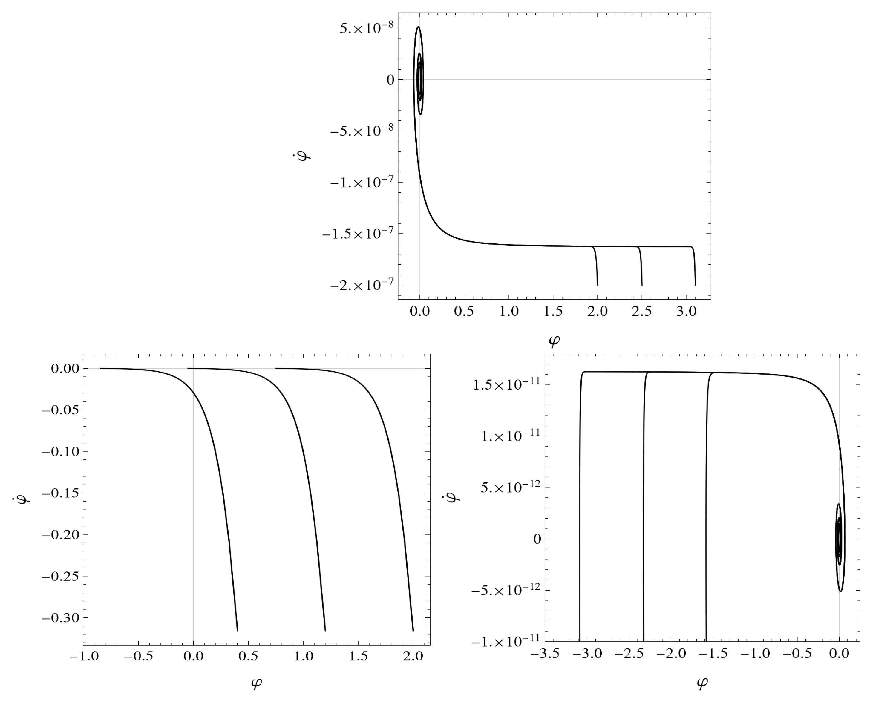
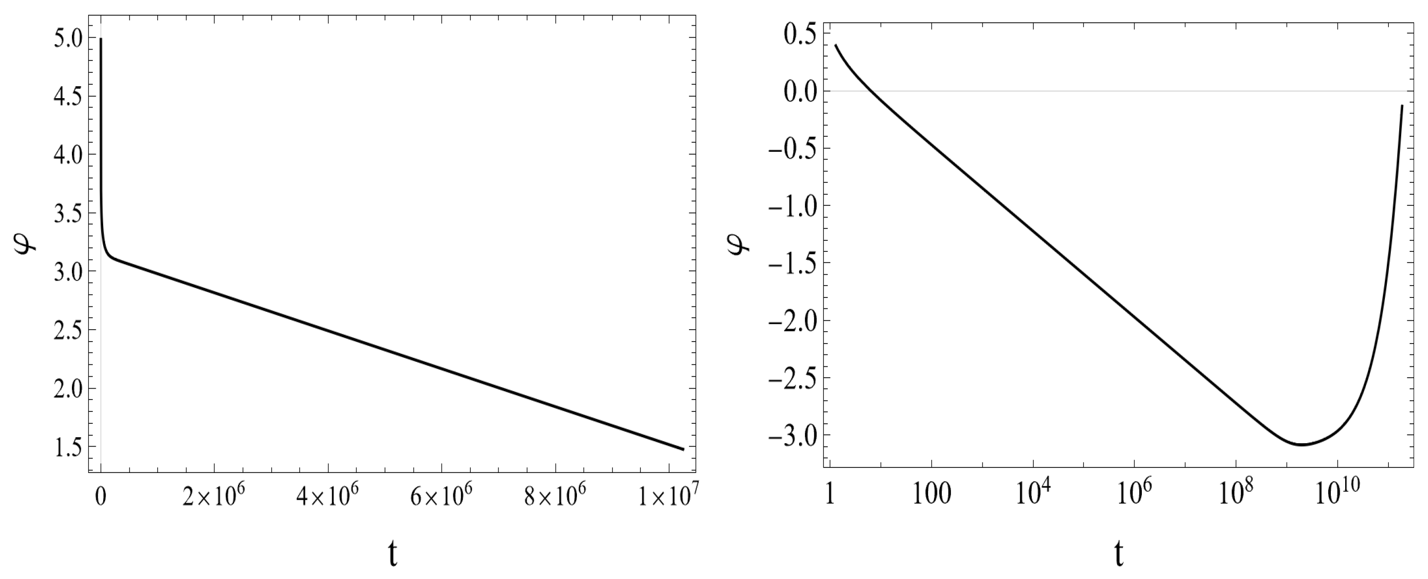
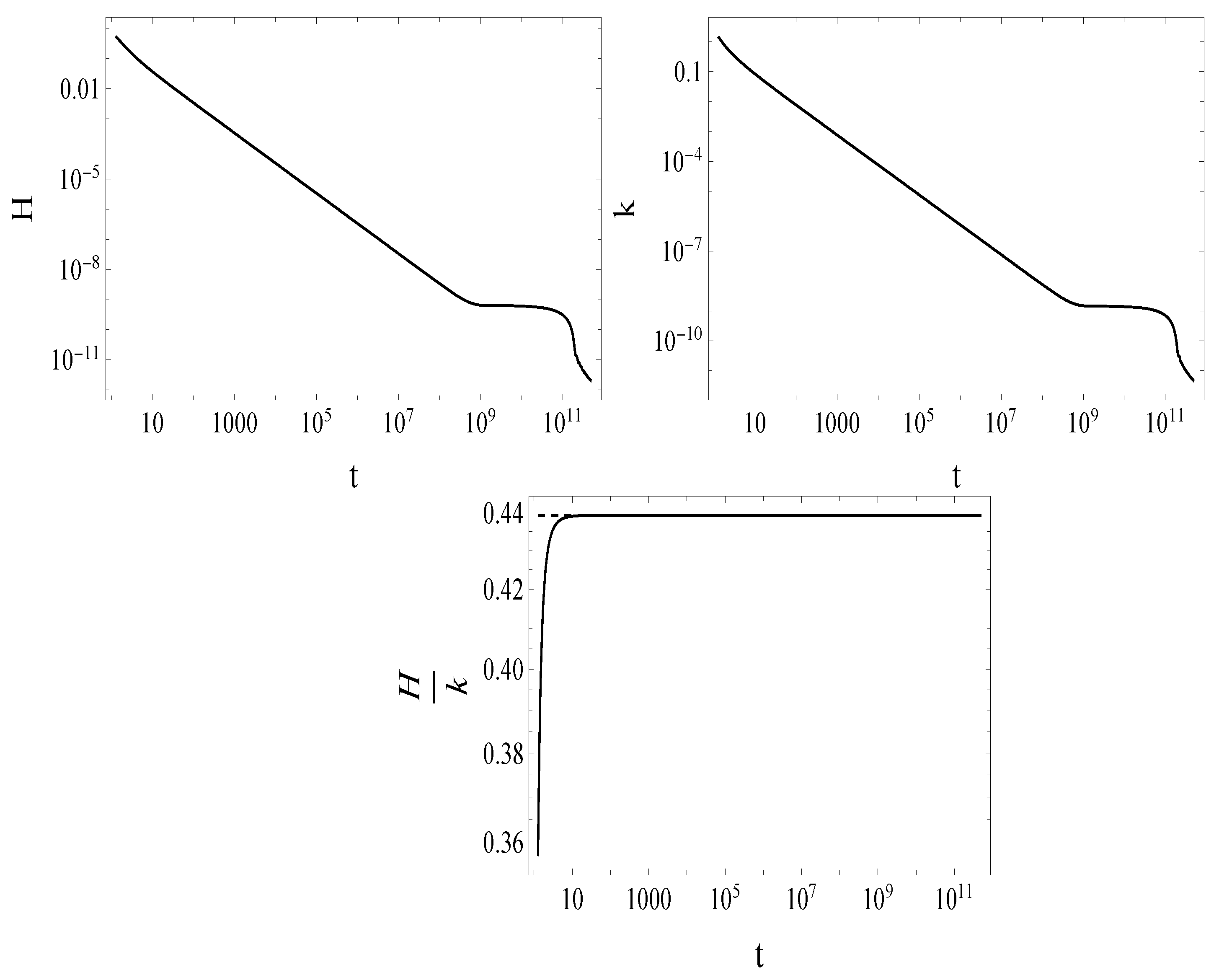
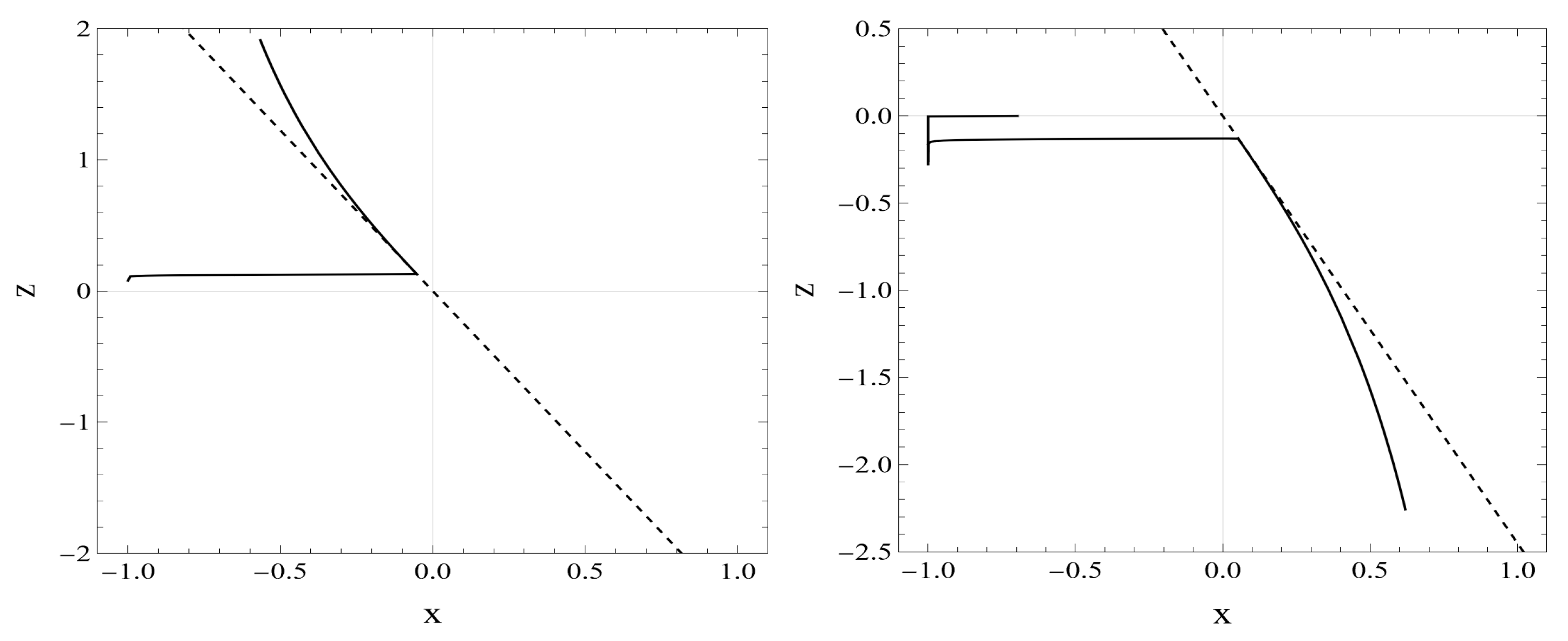
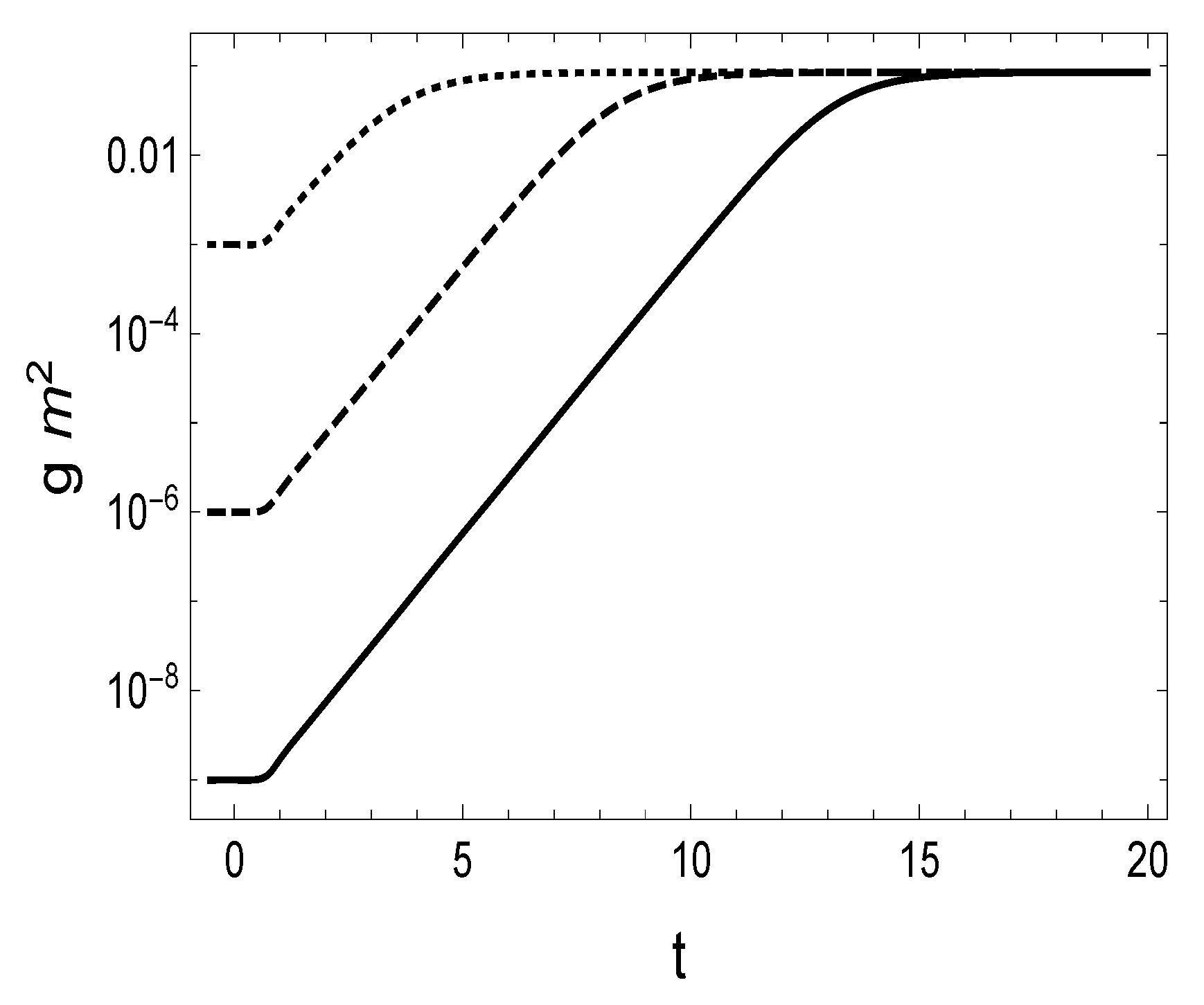
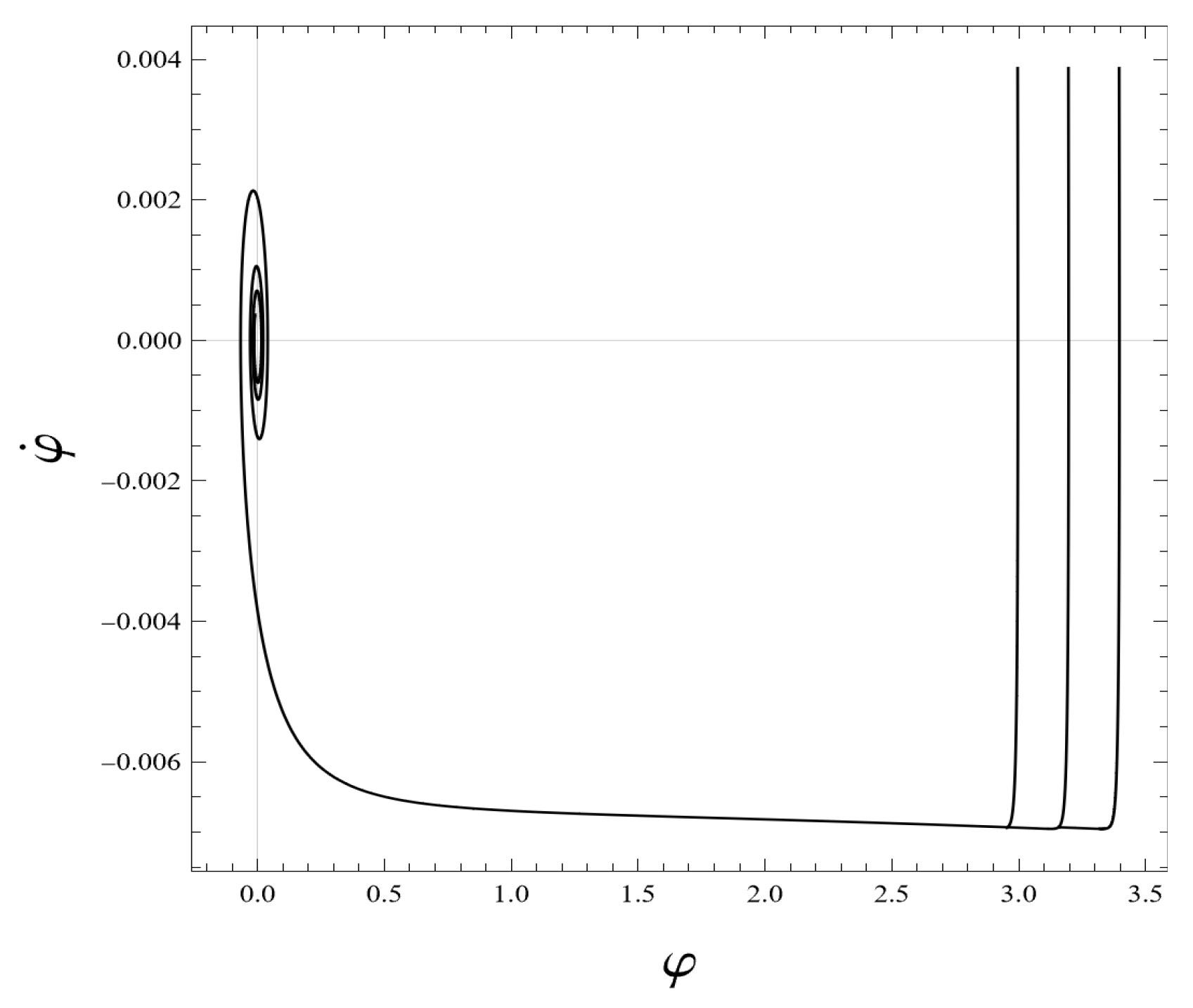
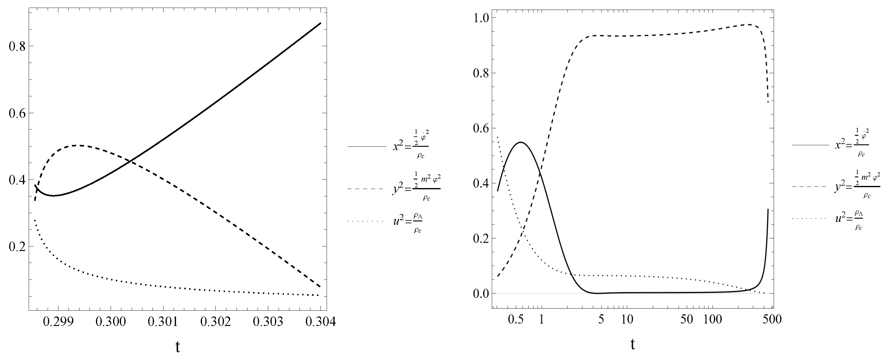
• As shown in Figure 1 (the bottom plot to the right), the phase trajectories run onto the universal attractor (with ${\dot{\phi }}_{\mathrm{attractor}}^{\text{QIM1}}\approx 1.6\times {10}^{-11}{m}_{\mathrm{Pl}}^2$ for $m^{\text{QIM1}}={10}^{-10}{m}_{\mathrm{Pl}}$) even in the quantum-improved case. In QIM1, the desirable slow-roll inflation sets on at the scale $k_i\sim {10}^{-9}{k}_G$. Therefore, as we argued in Appendix B, the quantum-improved attractor given by Equation (A14) is practically the same as the classical attractor given by Equation (A20), except for the big difference in the numerical values of the inflaton masses in QIM1 and GRM. Nevertheless, there is a difference in the evolution of the system in the classical GRM and in QIM1 that can be explained by the time dependence of the field $\phi$ in both cases, shown in Figure 2. Along the classical trajectory, the magnitude of the inflaton field $\left|\phi \right|$ decreases strictly monotonically up to the end of the slow-roll era and $\phi$ starts to oscillate around zero afterward for $t>t_f$. On the plot to the left in Figure 2, it is well distinguishable the preinflationary era with a rather steep fall off of $\left|\phi \right(t\left)\right|$ followed by the slow-roll era, with an almost linear decrease of $\left|\phi \right(t\left)\right|$ with increasing time t (c.f. Equation (A20)), both well known [58]. The plot to the right in Figure 2 shows the time dependence of $\phi \left(t\right)$ in QIM1. In RFPE (with $\phi \left(t\right)>0$) for $t\le t_G\approx 1.27$ $s_{\mathrm{Pl}}$ the evolution of the system can be estimated as given in Appendix A; the gravitational couplings evolve according to the scaling laws dictated by the Reuter FP, and the scalar field exhibits an ultrahard EoS. Just after the end of RFPE, $\phi \left(t\right)$ crosses zero at $t=t_{\times }$ ($t_{\times }\approx 6.3$ $s_{\mathrm{Pl}}$ on the plot). With the start of COE2, the scaling laws of the gravitational couplings alter: according to Equations (3) and (4), $G\left(k\right)\approx G_0$ raises slightly, keeping its order of magnitude, while $\Lambda \left(k\right)$ falls off proportionally with $k^4$. This implies that the yet huge kinetic energy density of the scalar field increases further at the cost of the dark energy density falling off proportionally to $k^4$ (see the plot to the left on Figure 3). Therefore, the field $\phi \left(t\right)$ continues to decrease through negative values and runs up the potential $U\left(\phi \right)$ on the other side, where it reaches the turning point at ${\phi }_{\mathrm{t}.\mathrm{p}.}\approx -3.1m_{\mathrm{Pl}}$ at the time $t=t_{\mathrm{t}.\mathrm{p}.}\approx 2\times {10}^9$ $s_{\mathrm{Pl}}$, where $\left|\phi \right|$ takes its maximum value and the inflaton field loses its kinetic energy density, terminating the preinflationary era. Reaching the turning point of $\phi$ is preceded by getting equal the fraction of the kinetic energy density ${\dot{\phi }}^2/2$ and that of the potential energy density $U\left(\phi \right)$ to the critical energy density (the point of the equality $x^2={\underset{¯}{y}}^2$ lies at $t_{\mathrm{xy}}\approx 4.8\times {10}^8$ $s_{\mathrm{Pl}}$ on the plot to the left in Figure 3). Rather soon after the turning point, the slow roll sets on, i.e., $t_{\mathrm{t}.\mathrm{p}.}\lesssim t_i$. Then an almost linear decrease of $\left|\phi \right(t\left)\right|$ takes place (c.f. Equation (A20)), followed by the damped oscillations of the field $\phi \left(t\right)$ for $t>t_f$, like in the classical case.
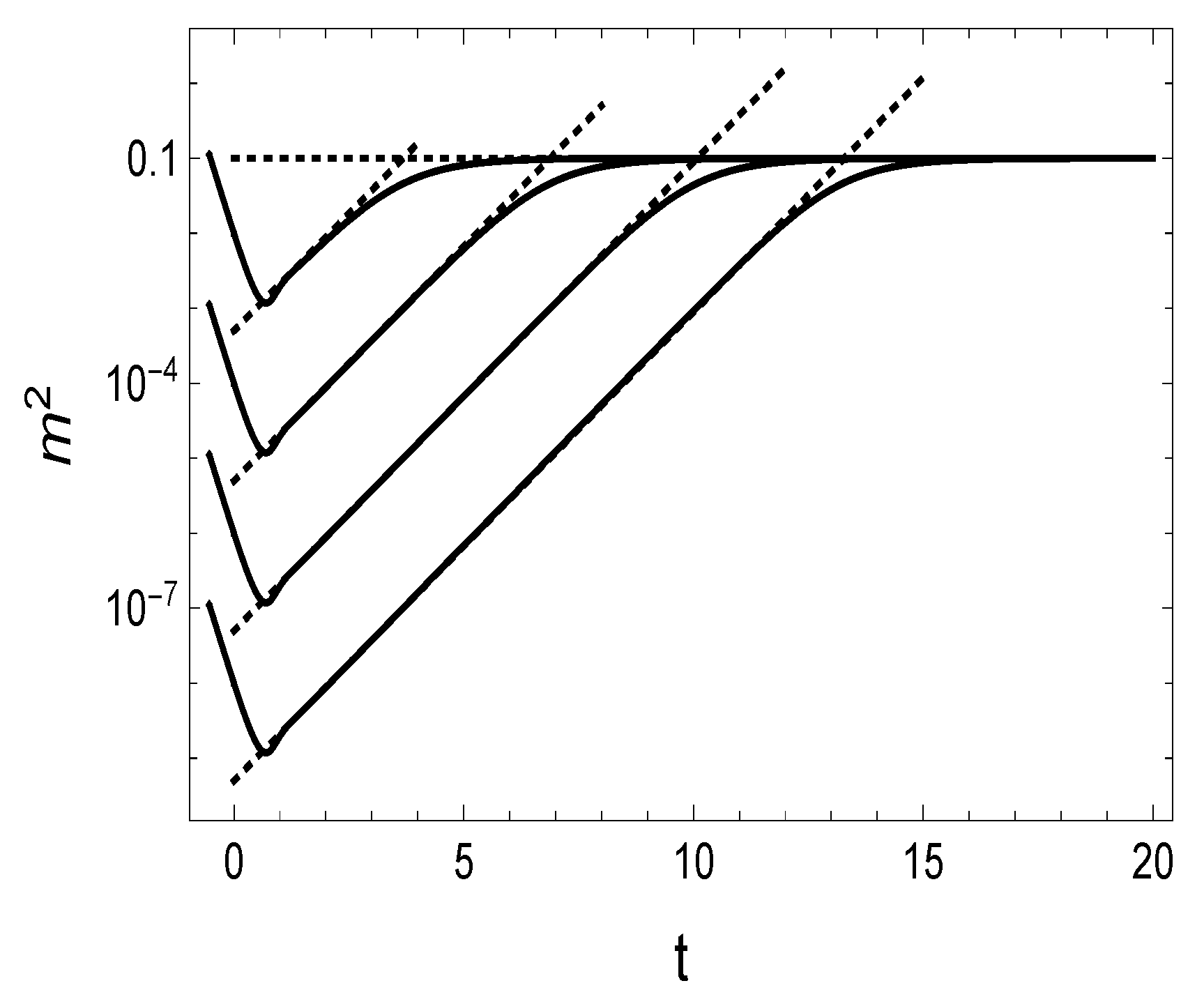
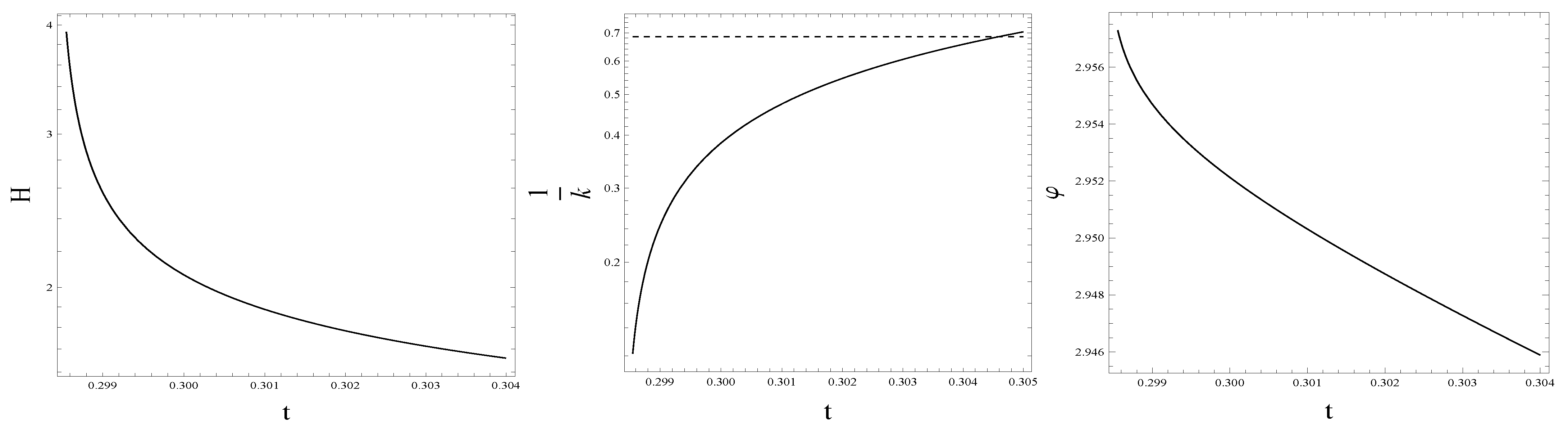
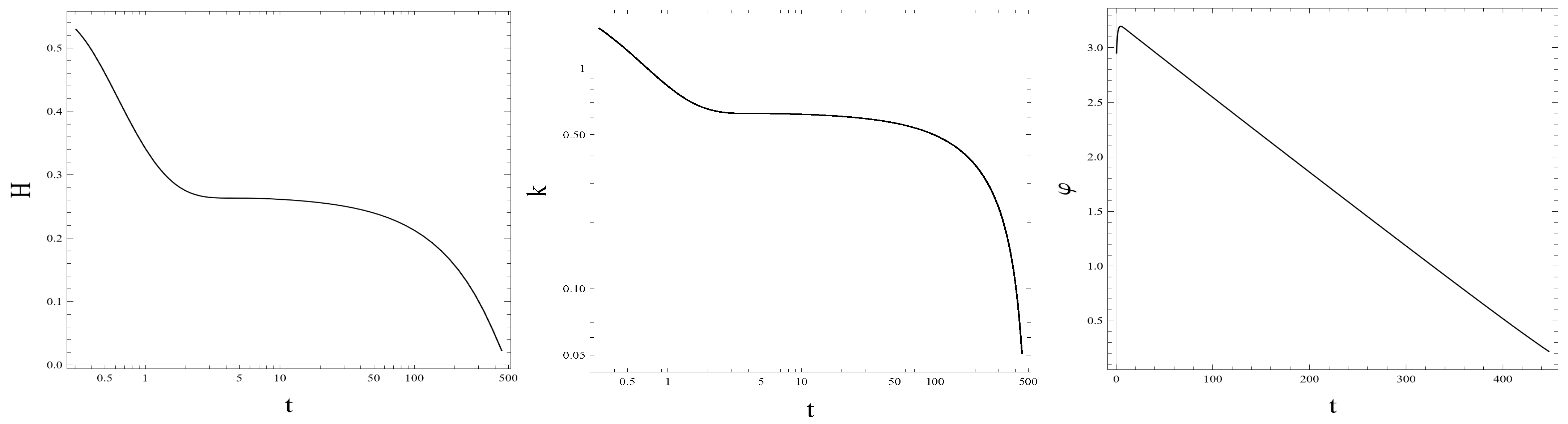
• The plots on the top of Figure 4 show that the Hubble parameter H and the energy scale k exhibit quite similar time dependences: both of them suffer a fall off of roughly eight orders of magnitude during the preinflationary era followed by a rather slow (less than an order of magnitude) decrease during the slow roll era. In the preinflationary era, except for its very beginning and very end, the potential energy density $U_k\left(\phi \right)$ and the dark energy density ${\rho }^{(\Lambda )}$ are negligible as compared with the kinetic energy density ${\dot{\phi }}^2/2$ (see the plot to the left in Figure 3), and it holds $G\left(k\right)\approx G_0$. Therefore, the Friedmann equations reduce to the ones

  $$\begin{array}{ccc}& & 3H^2\approx 4\pi G_0{\dot{\phi }}^2,\dot{H}\approx -4\pi G_0{\dot{\phi }}^2\hfill \end{array}$$

  (31)

  providing the ODE $\dot{H}=-3H^2$ with the solution

  $$\begin{array}{ccc}\hfill H\left(t\right)& \approx & {\displaystyle \frac{H_{\times }}{1+3H_{\times }(t-t_{\times })}},\hfill \end{array}$$

  (32)

  where $H_{\times }=H\left(t_{\times }\right)$. This estimate fits the numerical results with better than a relative accuracy of $0.001$. Then one obtains

  $$\begin{array}{ccc}\hfill \dot{\phi }& \approx & -\sqrt{{\displaystyle \frac{3}{4\pi }}}H\left(t\right)m_{\mathrm{Pl}}\hfill \end{array}$$

  (33)

  and

  $$\begin{array}{ccc}\hfill \phi \left(t\right)& \approx & \phi \left(t_{\times }\right)-{\int }_{t_{\times }}^{t}d\underset{¯}{t}\dot{\phi }\left(\underset{¯}{t}\right)=\phi \left(t_{\times }\right)+\sqrt{{\displaystyle \frac{3}{4\pi }}}{m}_{\mathrm{Pl}}ln{\displaystyle \frac{H\left(t\right)}{H_{\times }}},\hfill \end{array}$$

  (34)

  which states that the field amplitude decreases roughly proportionally with the logarithm of the time $0\lesssim t-t_{\times }\lesssim t_i-t_{\times }$ the system spent in the preinflationary era (as shown on the plot to the right in Figure 2). Approaching the end of the preinflationary era, the increasing fraction ${\underset{¯}{y}}^2=U_k\left(\phi \right)/{\rho }_c$ of the potential energy density becomes equal to the decreasing fraction $x^2=({\dot{\phi }}^2/2)/{\rho }_c$ of the kinetic energy density of the inflaton field at times $t_{\mathrm{xy}}\approx 4.8\times {10}^8$ $s_{\mathrm{Pl}}$, and this precedes the onset of the slow roll energetically with some delay at $t=t_i^{\text{QIM1}}$ (see the plot to the left in Figure 3).
  It is argued in Appendix D that in the slow-roll inflationary era, the Hubble parameter should show a rather slight linear decrease with increasing cosmological time t. It has been found that the numerically evaluated value of the Hubble parameter H is in a few percentage agreement with the value $H^{\mathrm{sl}.\mathrm{r}.}$ obtained from the analytical Formula (A21), except at the very end of the slow-roll era.
  As it is shown on the plot on the bottom of Figure 4, the ratio $H/k$ is constant for $t_{\times }\lesssim t\le t_f$ except for the rather short time interval $t_G\le t\lesssim t_{\times }$ lasting from the beginning of the preinflationary era to the zero-crossing time of $\phi$. Except for the latter time interval, it holds the relation $H=\sqrt{{\lambda }_{\ast }}k$ (shown by the dashed line on the plot) with good accuracy. Let us insert the expression of ${\rho }^{\left(\phi \right)}$ given by the reduced consistency condition (22) and ${\rho }^{(\Lambda )}$ as given in Equation (9) into the first Friedmann Equation (7), make the approximation $G\left(k\right)\approx G_0$, and neglect the term $F\ll k^4$ in Equation (4); then we find that

  $$\begin{array}{ccc}\hfill H^2& \approx & {\lambda }_{\ast }{k}^2\left(1-{\displaystyle \frac{k^2}{3k_G^2}}\right),\hfill \end{array}$$

  (35)

  which yields the estimate $H\approx \sqrt{{\lambda }_{\ast }}k$ for $k\ll k_G$ with good accuracy, in agreement with the result of numerics. The ratio $H/k\approx H^{\left(\mathrm{est}\right)}/k^{\left(\mathrm{est}\right)}=\sqrt{2{\lambda }_{\ast }/3}$ is somewhat smaller in RFPE than its value in the preinflationary and inflationary eras; its increase happens during the short time interval $t_G\le t\lesssim t_{\times }$.
• The various time dependences $H=2/\left(3t\right)$ (see Equation (A4) in Appendix A), $H={\displaystyle \frac{H_{\times }}{1+3H_{\times }(t-t_{\times })}}$ (see Equation (32)), and $H=H\left(t_f\right)+{\displaystyle \frac{m^2}{3}}(t_f-t)$ (see Equation (A21) in Appendix D) of the Hubble parameter in RFPE, the preinflationary, and slow-roll inflationary eras, respectively, inform one on the time dependence of the scale factor,

  $$\begin{array}{ccc}\hfill a\left(t\right)& \propto & \{\begin{array}{ccc}{t}^{2/3}& & \mathrm{RFPE}\\ {\left(1+H_{\times }(t-t_{\times })\right)}^{1/3}& & \mathrm{preinflationary}\mathrm{era}\\ exp\left[\left(H\left(t_f\right)+{\displaystyle \frac{m^2}{3}}{t}_f\right)t-{\displaystyle \frac{m^2}{6}}{t}^2\right]& & \mathrm{inflationary}\mathrm{era}\end{array}\hfill \end{array}$$

  (36)

  and on that of the deceleration parameter

  $$\begin{array}{ccc}\hfill q\left(t\right)& =& -{\displaystyle \frac{a\ddot{a}}{{\dot{a}}^2}}=-1-{\displaystyle \frac{\dot{H}}{H^2}}=\{\begin{array}{ccc}1/2& & \mathrm{RFPE}\\ 2& & \mathrm{preinflationary}\mathrm{era}\\ -1+\epsilon \left(t\right)& & \mathrm{inflationary}\mathrm{era}\end{array}.\hfill \end{array}$$

  (37)
  Thus, one finds that the quantum gravitational effects, being strong in the Reuter FP driven and the preinflationary eras, do not result in the accelerating expansion of the universe; the latter occurs due to the presence of the inflaton field in the slow-roll era, with the characteristic value of the deceleration parameter $q\left(t_i^{\text{QIM1}}\right)\approx -1+\epsilon \left(t_i^{\text{QIM1}}\right)=-0.998$, which corresponds to an almost exponential increase of the scale factor $a\left(t\right)$. It is worthwhile mentioning that in RFPE the scalar field behaves like dust so far as the time dependence of the scale factor $a\propto t^{2/3}$ is considered, which is the consequence of the interplay between the ultrahard EoS and the Reuter FP governed scaling laws of the gravitational couplings (see Appendix A).
• It has been shown that the slow-roll inflationary era occurs inside COE2 for a wide range of the inflaton mass m. In

  Table 1. Beginning $t_i$ and end $t_f$ of the slow-roll era, and the number $\underset{,}{\mathrm{N}}$ of e-foldings for various inflaton masses m in QIM1.

  $\mathit{m}/{\mathit{m}}_{\mathbf{Pl}}$	${\mathit{t}}_{\mathit{i}}$$\left({\mathbf{s}}_{\mathbf{Pl}}\right)$	${\mathit{t}}_{\mathit{f}}$$\left({\mathbf{s}}_{\mathbf{Pl}}\right)$	$\mathcal{N}$
  ${10}^{-13}$	$1.72\times {10}^{12}$	$2.47\times {10}^{14}$	110
  ${10}^{-12}$	$2\times {10}^{11}$	$2.25\times {10}^{13}$	92
  ${10}^{-11}$	$2.26\times {10}^{10}$	$2.04\times {10}^{12}$	75
  ${10}^{-10}$	$2.3\times {10}^9$	$1.84\times {10}^{11}$	60
  ${10}^{-9}$	$2.25\times {10}^8$	$1.6\times {10}^{10}$	47
  ${10}^{-8}$	$2.55\times {10}^7$	$1.38\times {10}^9$	36
  ${10}^{-7}$	$3.3\times {10}^6$	$1.17\times {10}^8$	26
  ${10}^{-6}$	$3.3\times {10}^5$	$9.7\times {10}^6$	18

  , one can see that the onset time $t_i$ of the slow roll is shifted to later times, and the duration of the slow-roll era becomes longer by a few orders of magnitude when the inflaton mass decreases from ${10}^{-6}{m}_{\mathrm{Pl}}$ to ${10}^{-13}{m}_{\mathrm{Pl}}$ while the number $\underset{,}{\mathrm{N}}$ of e-foldings rises within an order of magnitude.
• Comparing the time scales of the desirable slow-roll inflation given in Equation (28) for QIM1 with those for the classical model, GRM, given in Equation (25), one sees that there are (i) four orders of magnitude time delay in the start and (ii) also four orders of magnitude increase of the duration of the desirable slow-roll inflation due to the quantum gravitational effects. At around the scale $k_G$ (at the time $t_G$), the running Newton coupling $G\left(k\right)$ rather suddenly reaches its classical value $G_0$, while the running cosmological constant is yet huge (of the order of $k_G^4$) at that scale and decreases only slowly with decreasing scale k. This circumstance hinders the inflaton field from losing its kinetic energy density as fast as in the classical case. Furthermore, as it is seen in the plots in Figure 2, the desirable slow roll starts roughly at the same value of $\left|\phi \right(t_i\left)\right|$ in the classical and the quantum-improved cases, but the corresponding potential energy density in the quantum-improved case is eight orders of magnitude less than in the classical case due to the change in the required value of $m^2$. This is another reason that much more time is needed for the potential energy density to take over the kinetic energy density of the inflaton field in the quantum-improved case. In spite of the different timing of the slow roll in GRM and QIM1, the main qualitative features of the slow-roll inflation are negligibly affected by the quantum effects, except for the amplitude $A_s$ for the scalar perturbations, as discussed in Appendix D on the level of analytic estimates. A comparison of our numerical results, obtained for the desirable slow roll, given in Equations (26) and (27) for GRM and in Equations (29) and (30) for QIM1, completely supports the expectation that only the amplitude of the scalar perturbations is affected significantly by the quantum improvement. The reason is the rather small inflaton mass $m^{\text{QIM1}}\sim \mathcal{O}\left({10}^{-10}{m}_{\mathrm{Pl}}\right)$ required to achieve the desirable number $\underset{,}{\mathrm{N}}\approx 60$ of e-foldings. Maybe accidentally, GRM yields better, an order-of-magnitude agreement of $A_s$ with the observational data given in Refs. [61,62], than QIM1. Therefore, one has to conclude that the simple inflaton potential $U=m^2{\phi }^2/2$ with scale-independent inflaton mass works much worse in the quantum-improved case than in the classical one.

3.3. Evolution in Terms of the Dimensionless Quantities

3.3.1. General Considerations

In the present section we reexpress our numerical results in terms of the dimensionless cosmological variables [1,56,57]. This enables us to identify the cosmological fixed point (CFP) corresponding to RFPE, identify in another way the section of the phase trajectory along which the slow-roll inflation takes place, and get more insight into the changes in the energetic relations during the evolution. Instead of depicting the phase trajectories on the plane $(\phi ,\dot{\phi })$ one can follow them up on the plane $(x,z)$ by making use of the dimensionless quantities defined in the same manner as in Ref. [1]:

$$\begin{array}{ccc}\hfill & & x=\pm \sqrt{{\displaystyle \frac{{\dot{\phi }}^2/2}{{\rho }_c}}},y=+\sqrt{{\displaystyle \frac{{\rho }^{(\Lambda )}+U_k\left(\phi \right)}{{\rho }_c}}},z={\displaystyle \frac{U_{k,\phi }\left(\phi \right)}{\kappa [{\rho }^{(\Lambda )}+U_k\left(\phi \right)]}},\hfill \end{array}$$

(38)

where the critical density is given as ${\rho }_c=3H^2/{\kappa }^2$. Then, it holds the equality $y^2={\underset{¯}{y}}^2+u^2$. For flat spatial geometry, the critical density is equal to the total energy density, i.e., it holds ${\rho }_c=({\dot{\phi }}^2/2)+U_k\left(\phi \right)+{\rho }^{(\Lambda )}$, implying the constraint $x^2+y^2=1$. The idea behind the definitions (38) is that the dark energy density ${\rho }^{(\Lambda )}$ is considered to be the field-independent piece of the potential energy density of the scalar field.

In the classical case, in GRM, the dark energy density ${\rho }_0^{(\Lambda )}={\Lambda }_0/\left(8\pi G_0\right)$ and the potential energy density $U\left(\phi \right)$ are negligible as compared with the kinetic energy density of the inflaton field in the limit $t\to 0$, so that it holds $y^2\ll x^2$ and the variable x should tend to one of the values $x_{\ast }^{\mathrm{cl}.}=\pm 1$. Since $\left|\phi \right|\to \infty$ in the limit $t\to 0$, the dark energy density is negligible as compared with the potential energy density $U\left(\phi \right)$, and the variable $z\approx 2/\left(\kappa \phi \right)$ should vanish, i.e., $z_{\ast }^{\mathrm{cl}.}=0$ according to the definitions (38). The physically relevant phase trajectory starts indeed from the CFP $(x_{\ast }=-1,z_{\ast }=0)$ on the top left plot in Figure 5. As to QIM1, we have shown above, in terms of the dimensionful variables, that the evolution in RFPE can be very accurately estimated analytically. Making use of the estimates derived in Appendix A, one obtains the following estimates for the dimensionless variables (38):

• The variable $x\left(t\right)$ keeps strictly one of the constant values

  $$\begin{array}{ccc}\hfill x^{\left(\mathrm{est}\right)}\left(t\right)& =& {\displaystyle \frac{\kappa \dot{\phi }}{\sqrt{6}H}}{|}^{\left(\mathrm{est}\right)}=\pm {\displaystyle \frac{1}{\sqrt{2}}}\equiv x_{\ast }\hfill \end{array}$$

  (39)

  in RFPE. Since $H\propto k$ (see Appendix A), it holds

  $$\begin{array}{ccc}\hfill {\displaystyle \frac{dlnk}{dN}}& =& {\displaystyle \frac{dlnH}{dN}}=3x_{\ast }^2,\hfill \end{array}$$

  (40)

  implying that $k\propto e^{3N/2}$ in RFPE. (Here, we made use of eq. (27) in Ref. [1] applied to our case.) This means that $k\to \infty$ in the limit $N\to \infty$, i.e., in the limit $a\to 0$ ($t\to 0$). Therefore, the CFP corresponding to the Big Bang continues to evolve with the scale factor a.
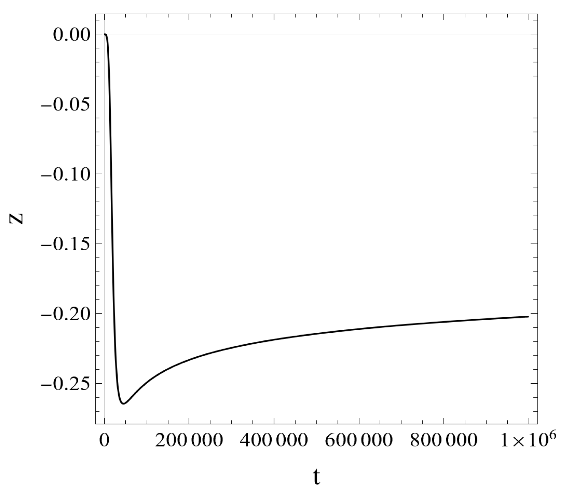
• In RFPE, $U\left(\phi \right)$ is negligible as compared with ${\rho }^{(\Lambda )}$, $0<U\left(\phi \right)\ll {\rho }^{(\Lambda )}$, so that one finds

  $$\begin{array}{ccc}\hfill & & z^{\left(\mathrm{est}\right)}\approx {\displaystyle \frac{m^2\phi }{\kappa {\rho }^{(\Lambda )}}}{|}^{\left(\mathrm{est}\right)}\stackrel{N\to \infty }{\sim }{\displaystyle \frac{m^2\sqrt{8\pi g_{\ast }}}{{\lambda }_{\ast }}}{\displaystyle \frac{\phi }{k^3}}{|}^{\left(\mathrm{est}\right)}\sim \mp \sqrt{3}{m}^2{t}^2\to 0^{\mp }.\hfill \end{array}$$

  (41)
  The variable z shows up time dependence (N-dependence) in RFPE, but it tends to zero in the limit $t\to 0$.

Therefore, we conclude that the pair of the CFPs corresponding to the various signs of the scalar field amplitude $\phi$ at the Big Bang singularity are at

$$\begin{array}{ccc}& & x_{\ast }^{\text{QIM1}}=\pm {\displaystyle \frac{1}{\sqrt{2}}},z_{\ast }^{\text{QIM1}}=0.\hfill \end{array}$$

(42)

The CFPs appear to belong to the limit $k\to \infty$. On the top right plot in Figure 5, the phase trajectory runs out from such a CFP, indeed, and RFPE is represented by the straightline section $x=-1/\sqrt{2}$ and $0\le z\left(t\right)\lesssim \sqrt{3}{m}^2{t}_G^2\approx 3\times {10}^{-20}$ being compressed to the single point of the CFP on the plot.

In order to find the characteristics of the section of the phase trajectory in the slow-roll era for QIM1, let us neglect the kinetic energy density term on the right-hand side of the first Friedmann Equation (7) and the term $\ddot{\phi }$ on the left-hand side of the Klein–Gordon Equation (11), multiply both sides of Equation (11) by $\dot{\phi }$, and divide both sides of both equations by ${\rho }_c$, then one obtains

$$\begin{array}{ccc}\hfill 1& \approx & y^2,\hfill \end{array}$$

(43)

$$\begin{array}{ccc}\hfill x(\sqrt{6}x+y^{2}z)& \approx & 0,\hfill \end{array}$$

(44)

where we have used the definition of the variable z in (44). Supposing that $x\not\equiv 0$ in the slow-roll era, one finds

$$\begin{array}{ccc}\hfill \sqrt{6}x+z& \approx & 0.\hfill \end{array}$$

(45)

This determines the straightline section on the $(x,z)$ plane along which the system evolves during the slow-roll inflation both in the classical and quantum-improved cases [1].

3.3.2. Numerical Results

The numerically obtained phase trajectories providing the desirable slow-roll inflation are shown on the $(x,z)$ plane in Figure 5 for GRM and QIM1.

As shown on the top left plot in Figure 5, in the classical case, i.e., for GRM, the phase trajectory providing the desirable slow-roll inflation runs out of the CFP at $(x_{\ast }^{\mathrm{cl}.}=-1,z_{\ast }^{\mathrm{cl}.}=0)$. Just after the Big Bang. the ultrahard EoS of the inflaton field implies the time dependences ${\dot{\phi }}^2/2\propto t^{-2}$, $\left|\phi \right|\propto -|lnt|$ [58]; furthermore, the kinetic energy density of the inflaton field dominates completely over its potential energy density $U\left(\phi \right)$ and the dark energy density ${\rho }_0^{(\Lambda )}$. Therefore, it holds $x\left(t\right)\approx -1$, while $z\left(t\right)\approx {\displaystyle \frac{2}{{\kappa }_0\phi }}$ increases slowly with the logarithmic fall off of $\left|\phi \right|$. The era characterized by the ultrahard EoS is represented on the plot by the vertical section of the phase trajectory running out of the CFP. At its end, the potential energy density $m^2{\phi }^2/2$ becomes comparable to the kinetic energy density, and the phase trajectory starts to run towards the slow-roll line with a sudden fall off of $\left|x\right|$ while $\left|z\right|$ ($\left|\phi \right|$) increases (decreases) negligibly (the horizontal piece of the phase trajectory on the plot). The dominance having taken by the potential energy density $m^2{\phi }^2/2$ over the kinetic energy density ${\dot{\phi }}^2/2$, the slow roll sets on and the phase trajectory runs tangentially to the slow-roll line, deviating from it finally at the end of the slow-roll era. Up to the end of the slow-roll era, the dark energy density ${\rho }_0^{(\Lambda )}$ does not play any role in the classical case due to the extremely small value of the cosmological constant ${\Lambda }_0$. The $(x,z)$ plot stretches out the piece of the phase trajectory between the end of the ultrahard EoS-driven evolution and the onset of the slow-roll separated in cosmological time by much less than an order of magnitude change.

The top right plot in Figure 5 shows the phase trajectory providing the desirable slow-roll inflation in QIM1. Here the vertical section (reduced to the CFP on the plot) at $x_{\ast }^{\text{QIM1}}=-1/\sqrt{2}$ with rather small values of $z\left(t\right)\ge 0$ suppressed by $m^2$ (see Equation (41)) represents in a compressed manner the whole evolution in RFPE when the potential energy density $m^2{\phi }^2/2$ is negligible and the density of the dark energy and that of the kinetic energy of the scalar field are equal and both falling off proportionally to $k^4$, ${\rho }^{(\Lambda )}={\displaystyle \frac{1}{2}}{\dot{\phi }}^2\propto k^4$ due to the constraint (17). Till the end of the slow roll, the phase trajectory has several turning points on the $(x,z)$ plane: due to the zero-crossing of $\phi$ at $t=t_{\times }\approx 6.3$ $s_{\mathrm{Pl}}$, at $t=t_{\mathrm{z}}\approx 5\times {10}^4$ $s_{\mathrm{Pl}}$ when $\left|z\right|$ takes its maximum value (see Figure 6), at $t=t_{\mathrm{t}.\mathrm{p}.}\approx 2.0\times {10}^9$ $s_{\mathrm{Pl}}$ when $\left|\phi \right|$ takes its maximum value, and at $t=t_i\approx 2.3\times {10}^9$ $s_{\mathrm{Pl}}$ due to the onset of the slow roll. Just after the end of RFPE for $t_G\lesssim t\lesssim t_{\times }$, the fraction of the kinetic energy density of the inflaton field and that of the dark energy density in ${\rho }_c$ behave approximately as

$$\begin{array}{ccc}\hfill & & x^2={\displaystyle \frac{{\dot{\phi }}^2/2}{{\rho }_c}}\approx {\displaystyle \frac{{\dot{\phi }}^2/2}{{\dot{\phi }}^2/2+{\rho }^{(\Lambda )}}}\approx {\displaystyle \frac{1}{1+\xi \left(k\right)}}\mathrm{and}{u}^2={\displaystyle \frac{{\rho }^{(\Lambda )}}{{\rho }_c}}\approx {\displaystyle \frac{{\rho }^{(\Lambda )}}{{\dot{\phi }}^2/2+{\rho }^{(\Lambda )}}}\approx {\displaystyle \frac{\xi \left(k\right)}{1+\xi \left(k\right)}}\mathrm{with}\xi \left(k\right)={\displaystyle \frac{k^2}{-2k^2+3k_G^2}},\hfill \end{array}$$

(46)

respectively, since ${\overline{y}}^2=U_k\left(\phi \right)/{\rho }_c$ is negligible, being much less than $x^2$ and $u^2$. The denominator of $\xi \left(k\right)$ in Equation (46) keeps its order of magnitude $\mathcal{O}\left(k_G^2\right)$ during the whole COE2 so that $\xi \left(k\right)$ falls off roughly proportionally to $k^2$. Then $u^2$ starts to fall off, x tends to the boundary value $-1$ (see also the plot to the left on Figure 3), while z slowly goes to zero through positive values. The corresponding piece of the phase trajectory is depicted by the upper left going horizontal linear section on the top right plot in Figure 5.

The evolution between the zero-crossing of $\phi$ at $t=t_{\times }$ and reaching by $\left|z\right|$ its maximum value at $t=t_{\mathrm{z}}$ is illustrated by the vertical down-going linear section on the top right plot on Figure 5. For $t_{\times }\ll t\lesssim t_{\mathrm{z}}$, the fraction of the dark energy density is already much less than that of the kinetic energy density of the inflaton field, $u^2\ll x^2$, but the falling off dark energy density becomes comparable with the increasing potential energy density $m^2{\phi }^2/2$ at $t=t_{\mathrm{yu}}\approx 2\times {10}^4$ $s_{\mathrm{Pl}}$, although the latter is yet much less than the kinetic energy density ${\dot{\phi }}^2/2$ (see the plots in Figure 3). Since there hold the estimates $G\approx G_0$ and $\Lambda \approx c{k}^4$ in that time interval, one obtains ${\rho }^{(\Lambda )}\approx c{k}^4/\left(8\pi G_0\right)\approx {\lambda }_{\ast }{k}^4/\left(24\pi g_{\ast }\right)$ and

$$\begin{array}{ccc}\hfill z& \approx & {\displaystyle \frac{m^2\phi }{{\kappa }_0(\frac{{\lambda }_{\ast }}{24\pi g_{\ast }}{k}^4+\frac{1}{2}{m}^2{\phi }^2)}}.\hfill \end{array}$$

(47)

In the discussed time interval, k decreases closely inversely proportionally with t, while $\left|\phi \right|$ increases linearly with $lnt$ (c.f. Equation (34)). Therefore, so long ${\rho }^{(\Lambda )}$ dominates the denominator of z in Equation (47), its magnitude $\left|z\right|$ increases, but when the potential energy density becomes dominating, the variable z starts to approach the expression $2/\left({\kappa }_0\phi \right)$ and $\left|z\right|$ begins to decrease with increasing $\left|\phi \right|$. Therefore, the time $t=t_{\mathrm{z}}\approx 5\times {10}^4$ $s_{\mathrm{Pl}}$, at which $\left|z\right|$ takes its maximum value, is preceded by the time $t=t_{\mathrm{yu}}$. It is one of the advantages of plotting the phase trajectory on the $(x,z)$ plane that one becomes aware of the fact that the preinflationary era consists of 2 suberas: the one with $u^2>{\underset{¯}{y}}^2$ followed by another one with ${\underset{¯}{y}}^2>u^2$. These suberas are separated essentially by the maximum of the magnitude of the variable z.

In the time interval $t_{\mathrm{z}}\lesssim t\lesssim t_{\mathrm{t}.\mathrm{p}.}$ still hold the relations (46), the kinetic energy density of the scalar field still dominates over the potential energy density $m^2{\phi }^2/2$, i.e., $x^2\gg {\overline{y}}^2$, but the potential energy density $m^2{\phi }^2/2$ dominates already over the dark energy density, $m^2{\phi }^2/2\gg {\rho }^{(\Lambda )}$. Therefore, the variable z begins to behave like in the classical case, $z\approx 2/\left({\kappa }_0\phi \right)$, i.e., $\left|z\right|$ takes slowly decreasing values with logarithmically increasing $\left|\phi \right|$, while the variable x still takes values rather close to $-1$. This is illustrated by a vertically upgoing linear section of the phase trajectory on the top right plot in Figure 5. Then, approaching the turning point of $\phi$, i.e., for t approaching $t_{\mathrm{t}.\mathrm{p}.}$, the continuously rising potential energy density $m^2{\phi }^2/2$ becomes equal to the gradually decreasing kinetic energy density of the scalar field, $x^2=y^2$ at $t=t_{\mathrm{xy}}=5\times {10}^8$ $s_{\mathrm{Pl}}$ (see the plot to the left on Figure 3). The field $\phi$ moving uphill in the potential $U\left(\phi \right)$ slows down, and $x^2$ goes suddenly to zero, depicted by the bottom right going horizontal line on the top right plot in Figure 5. At $t=t_i$ the slow-roll sets on, and the phase point moves further along the slow-roll line running away from it when the end of the slow roll at $t=t_f$ is approached.

4. Scale-Dependent Inflaton Mass

4.1. Interpolation Formula for the Running Inflaton Mass

In the discussion above, the inflaton mass has been treated as a time-independent constant. The RG analysis of the EH gravity minimally coupled to the scalar field would yield, however, an RG flow of the inflaton mass. As it is mentioned in the Introduction, the authors of Ref. [50] thoroughly investigated the UV behavior of EH gravity coupled to a single real scalar field and established asymptotic safety of the model for the numbers of dimensions $d=3,4,5,6$. It has been shown that the Reuter FP exists for the number of dimensions $d=4$.

$$\begin{array}{ccc}\hfill {\Gamma }_k[g,\phi ]& =& \int d^{d}x\sqrt{g}\left(V\left({\phi }^2\right)-F\left({\phi }^2\right)R+{\displaystyle \frac{1}{2}}{g}^{\mu \nu }\partial {\phi }_{\mu }\partial {\phi }_{\nu }\right)+S_{\mathrm{GF}}+S_{\mathrm{gh}}\hfill \end{array}$$

(48)

for the Euclidean effective action, where V and F are polynomials of ${\phi }^2$, $S_{\mathrm{GF}}$ and $S_{\mathrm{gh}}$ stand for the gauge fixing and ghost terms, respectively, and $\sqrt{g}$ is the square root of the Euclidean metric $g_{\mu \nu }$. The DeDonder gauge has been chosen. The functional RG analysis has been performed by making use of the optimized cut-off [63,64] and solving Wetterich’s functional RG equation [65]. The explicit forms of the flow equations for the functions V and F are given in [50] and can be applied to our simple model with the massive, non-self-interacting scalar field minimally coupled to gravity. Our purpose is to find an overall picture of various scaling regimes of the mass parameter $m^2\left(k\right)$. Restricting ourselves to the case with $d=4$ and introducing the dimensionless quantities $\tilde{\phi }=k^{-1}\phi$, $\tilde{V}\left({\tilde{\phi }}^2\right)=k^{-4}V\left({\phi }^2\right)$, and $\tilde{F}\left({\tilde{\phi }}^2\right)=k^{-2}F\left({\phi }^2\right)$ and the truncated Taylor expansions $\tilde{V}\left({\tilde{\phi }}^2\right)={\sum }_{n=0}^1{\tilde{\lambda }}_{2n}{\tilde{\phi }}^{2n}$ and $\tilde{F}={\tilde{\xi }}_0$, we can apply the flow Equations (A1)–(A4) given in Appendix A in [50]. In terms of the dimensionless gravitational couplings $\tilde{g}=k^{2}G\left(k\right)$, $\tilde{\lambda }=k^{-2}\Lambda \left(k\right)$ and the dimensionless mass parameter $\tilde{m}=k^{-1}m$, they hold the correspondences

$$\begin{array}{ccc}& & {\tilde{\lambda }}_0\Rightarrow {\displaystyle \frac{\tilde{\lambda }}{8\pi \tilde{g}}},{\tilde{\lambda }}_2\Rightarrow {\displaystyle \frac{1}{2}}{\tilde{m}}^2,{\tilde{\xi }}_0\Rightarrow {\displaystyle \frac{1}{16\pi \tilde{g}}},\hfill \end{array}$$

(49)

which can be inverted as

$$\begin{array}{ccc}& & {\tilde{m}}^2=2{\tilde{\lambda }}_2,\tilde{g}={\displaystyle \frac{1}{16\pi {\tilde{\xi }}_0}},\tilde{\lambda }={\displaystyle \frac{{\tilde{\lambda }}_0}{2{\tilde{\xi }}_0}}.\hfill \end{array}$$

(50)

In the present section, we denote by tilde all dimensionless quantities, while in the other parts of the present paper, we use the notations g and $\lambda$ for the dimensionless gravitational couplings but keep the notation $\tilde{m}$ of the dimensionless inflaton mass. Moreover, in the present section, we use t to notate the "RG time” $t=ln(k/k_G)$. The flow Equations (A1), (A2) and (A3) taken from Ref. [50] (with ${\tilde{\xi }}_2={\tilde{\lambda }}_4=0$) are given as

$$\begin{array}{ccc}\hfill {\partial }_t{\tilde{\lambda }}_0& =& -4{\tilde{\lambda }}_0+{\displaystyle \frac{1}{32{\pi }^2}}\left[2+{\displaystyle \frac{1}{1+2{\tilde{\lambda }}_2}}+{\displaystyle \frac{6{\tilde{\lambda }}_0}{{\tilde{\xi }}_0-{\tilde{\lambda }}_0}}\right]+{\displaystyle \frac{\eta }{96{\pi }^2}}{\displaystyle \frac{5{\tilde{\xi }}_0-2{\tilde{\lambda }}_0}{{\tilde{\xi }}_0-{\tilde{\lambda }}_0}},\hfill \end{array}$$

(51)

$$\begin{array}{ccc}\hfill {\partial }_t{\tilde{\xi }}_0& =& -2{\tilde{\xi }}_0+{\displaystyle \frac{1}{384{\pi }^2}}\left[25-{\displaystyle \frac{4}{1+2{\tilde{\lambda }}_2}}+{\displaystyle \frac{8{\tilde{\xi }}_0(7{\tilde{\xi }}_0-2{\tilde{\lambda }}_0)}{{({\tilde{\xi }}_0-{\tilde{\lambda }}_0)}^2}}\right]+{\displaystyle \frac{\eta }{1152{\pi }^2}}{\displaystyle \frac{17{\tilde{\xi }}_0^2+18{\tilde{\xi }}_0{\tilde{\lambda }}_0-15{\tilde{\lambda }}_0^2}{{({\tilde{\xi }}_0-{\tilde{\lambda }}_0)}^2}},\hfill \end{array}$$

(52)

$$\begin{array}{cc}\hfill {\partial }_t{\tilde{\lambda }}_2=& -2{\tilde{\lambda }}_2+{\displaystyle \frac{1}{48{\pi }^2}}\left[{\displaystyle \frac{9{\tilde{\lambda }}_0}{2{({\tilde{\xi }}_0-{\tilde{\lambda }}_0)}^2}}-{\displaystyle \frac{9(2{\tilde{\lambda }}_0-{\tilde{\xi }}_0)}{2(1+2{\tilde{\lambda }}_2){({\tilde{\xi }}_0-{\tilde{\lambda }}_0)}^2}}-{\displaystyle \frac{9}{2{(1+2{\tilde{\lambda }}_2)}^2({\tilde{\xi }}_0-{\tilde{\lambda }}_0)}}\right]\hfill \\ & +{\displaystyle \frac{\eta }{96{\pi }^2}}\left[{\displaystyle \frac{3{\tilde{\xi }}_0}{2{({\tilde{\xi }}_0-{\tilde{\lambda }}_0)}^2}}-{\displaystyle \frac{3{\tilde{\xi }}_0}{2(1+2{\tilde{\lambda }}_2){({\tilde{\xi }}_0-{\tilde{\lambda }}_0)}^2}}\right],\hfill \end{array}$$

(53)

where $\eta =2+{\displaystyle \frac{{\partial }_t{\tilde{\xi }}_0}{{\tilde{\xi }}_0}}$. On the right-hand sides, singularity can occur for vanishing $1+2{\tilde{\lambda }}_2=1+{\tilde{m}}^2=0$ and ${\tilde{\xi }}_0-{\tilde{\lambda }}_0={\tilde{\xi }}_0(1-2\tilde{\lambda })=0$, i.e., for $\tilde{\lambda }=1/2$. The latter is the usual singularity when Litim’s cut-off is used.

It is straightforward to show, on the one hand, that there exists a class of solutions of the RG flow Equations (51)–(53) for which the mass parameter ${\tilde{\lambda }}_2$ vanishes identically. Namely, the flow Equation (53) is identically satisfied for identically vanishing ${\tilde{\lambda }}_2\left(k\right)\equiv 0$ for any solutions ${\tilde{\lambda }}_0\left(k\right)$ and ${\tilde{\xi }}_0\left(k\right)$ of Equations (51) and (52) (actually for any choice of the functions ${\tilde{\lambda }}_0\left(k\right)$ and ${\tilde{\xi }}_0\left(k\right)$). This means that the RG flow of pure EH gravity is a solution of the set of the flow Equations (51)–(53). Numerical investigation of the system of Equations (51)–(53) has revealed, on the other hand, that the RG flow has 3 FPs: the Gaussian FP at ${\tilde{g}}_{\ast }={\tilde{\lambda }}_{\ast }={\tilde{m}}_{\ast }^2=0$, and the non-Gaussian FPs NGFP₁ and NGFP₂ given in

Table 2. The non-Gaussian FPs in the space of the dimensionless couplings $({\tilde{g}}_{\ast },{\tilde{\lambda }}_{\ast },{\tilde{m}}_{\ast }^2)$ and their critical exponents $s_i$$(i=1,2,3)$.

	${\tilde{\mathit{g}}}_{\ast }$	${\tilde{\mathit{\lambda }}}_{\ast }$	${\tilde{\mathit{m}}}_{\ast }^2$	${\mathit{s}}_{1,2}$	${\mathit{s}}_3$
NGFP1	$0.846$	$0.176$	0.2	$-2.119\pm i2.878$	$-0.486$
NGFP2	$0.837$	$0.181$	0	$-2.143\pm i2.879$	$0.627$

. The study of the linearized RG equations at the non-Gaussian FPs yielded the critical exponents listed in Table 2. Thus, we have to conclude that NGFP₁ is the Reuter FP of the gravity–matter system being UV attractive and providing asymptotic safety, while NGFP₂ is the Reuter FP of the theory without matter (without the scalar field, i.e., the Reuter FP of pure EH gravity) representing a hyperbolic FP of the gravity-matter system, which is UV repulsive in the mass direction. The FP discussed by the authors of Ref. [50] and given in Table I of [50] for $d=4$ at ${\tilde{\lambda }}_0^{\ast }=8.620\times {10}^{-3}$, ${\tilde{\xi }}_0^{\ast }=2.375\times {10}^{-2}$ corresponds in our notations to ${\tilde{g}}_{\ast }=0,8376$ and ${\tilde{\lambda }}_{\ast }=0.1815$ and is identical with NGFP₂.

We chose NGFP₁ in our investigation since it, as opposed to NGFP₂, can make the model asymptotically safe. We also note that NGFP₂ provides an irrelevant direction in the evolution; therefore, it is not possible to reverse the direction of the numerical calculations for the trajectories. This implies that the trajectories should start in the close vicinity of the FP. However, the existing irrelevant direction and the elliptic nature of the FP disable one from fine-tuning the initial values of the couplings. Therefore, the trajectories starting from close to NGFP₂ cannot map out the vicinity of the Gaussian FP and cannot help us find the correct asymptotic behavior there. This issue does not appear in the case of NGFP₁, where we can start the evolution close to the Gaussian FP because the direction of the evolution can be reversed. By approaching the separatrix between the Gaussian FP and the Reuter FP, we can get the asymptotic scalings.

Restricting ourselves to the RG trajectories spiraling into NGFP₁ for $k\to \infty$, we have determined the dimensionless product $C\left(k\right)\equiv G\left(k\right)m^2\left(k\right)=\tilde{g}\left(k\right){\tilde{m}}^2\left(k\right)$ depicted in Figure 7. It has been established that the product $C\left(k\right)$ takes constant values $C_{\ast }={\tilde{g}}_{\ast }{\tilde{m}}_{\ast }^2$ and $C_0\equiv G_0{m}_0^2<C_{\ast }$ in the UV and IR regimes, respectively. In the far UV regime, the dimensionful mass squared is proportional to $k^2$, ${\tilde{m}}^2\left(k\right)={\tilde{m}}_{\ast }^2{k}^2$, and $C_{\ast }={\tilde{g}}_{\ast }{k}^{-2}{\tilde{m}}_{\ast }^2{k}^2={\tilde{g}}_{\ast }{\tilde{m}}_{\ast }^2$. The constant IR value $C_0$ occurs roughly at the RG scale $k\approx k_G$ when Newton’s coupling becomes constant, i.e., $C\left(k_G\right)\approx C_0$.

As shown in Figure 8, the RG flow of the mass squared ${\tilde{m}}^2$ reveals three scaling regions: (i) in the far UV ${\tilde{m}}^2$ tends to the constant value ${\tilde{m}}_{\ast }^2$ determined by the Reuter FP NGFP₁, (ii) for $k\lesssim k_G$ the IR scaling ${\tilde{m}}^2\propto k^{-2}$ yields the constant value $m_0^2$ of the dimensionful mass squared, and (iii) there occurs a crossover scaling region for $k_G\lesssim k\lesssim k_m$, where the power-law scaling $m^2\left(k\right)\propto k^{{\alpha }_m}$ of the dimensionful mass squared holds. The numerical fits (see the tilted dashed lines in Figure 8) yield the power ${\alpha }_m\approx 2.6$, independently of the value of $m_0^2$. The RG flow-generated scale $k_m$ has been determined numerically: we extrapolated the crossover scaling to the scale $k=k_m$ where it matches the constant UV value ${\tilde{m}}_{\ast }^2$ (see Figure 8). The result is shown in Figure 9 and has been fitted by

$$\begin{array}{ccc}\hfill {\lg }_{10}(k_m/k_G)& \approx & {\lg }_{10}{A}_m-{\beta }_m{\lg }_{10}(m_0^2/m_{\mathrm{Pl}}^2),\hfill \end{array}$$

(54)

so that we obtained

$$\begin{array}{ccc}\hfill k_m\left(m_0\right)& =& k_G{A}_m{(m_0/m_{\mathrm{Pl}})}^{-2{\beta }_m}\hfill \end{array}$$

(55)

with $A_m=6.7970\times {10}^{-2}$ and ${\beta }_m=0.694437$.

In order to reflect these properties of the function ${\tilde{m}}^2\left(k\right)$ in a qualitative manner, we treat $C_0=G_0{m}_0^2$, i.e., the IR value $m_0^2$ of the mass squared as a free parameter, and choose the interpolation formula

$$\begin{array}{ccc}\hfill m^2\left(k\right)& =& \{\begin{array}{ccc}{\tilde{m}}_{\ast }^2{k}^2& \mathrm{for}& k_m\le k\\ A{k}^{{\alpha }_m}+B& \mathrm{for}& k_G\le k\le k_m\\ m_0^2& \mathrm{for}& k\le k_G\end{array}\hfill \end{array}$$

(56)

where the constants A and B are determined by requiring continuity of $m^2\left(k\right)$ at $k=k_m$ and $k=k_G$,

$$\begin{array}{ccc}\hfill & & A={\displaystyle \frac{{\tilde{m}}_{\ast }^2{k}_m^2-m_0^2}{k_m^{{\alpha }_m}-k_G^{{\alpha }_m}}}={\tilde{m}}_{\ast }^2{k}_m^{2-{\alpha }_m}\left(1-{\displaystyle \frac{m_0^2}{{\tilde{m}}_{\ast }^2{k}_m^2}}\right){\left(1-{\displaystyle \frac{k_G^{{\alpha }_m}}{k_m^{{\alpha }_m}}}\right)}^{-1},\hfill \end{array}$$

(57)

$$\begin{array}{ccc}& & B={\tilde{m}}_{\ast }^2{k}_m^2-A{k}_m^{{\alpha }_m}={\tilde{m}}_{\ast }^2{k}_m^2\left({\displaystyle \frac{m_0^2}{{\tilde{m}}_{\ast }^2{k}_m^2}}-{\displaystyle \frac{k_G^{{\alpha }_m}}{k_m^{{\alpha }_m}}}\right){\left(1-{\displaystyle \frac{k_G^{{\alpha }_m}}{k_m^{{\alpha }_m}}}\right)}^{-1}\hfill \end{array}$$

(58)

This provides the RG parameter

$$\begin{array}{ccc}\hfill {\nu }_{RG}& =& {\beta }_{m^2}=\{\begin{array}{ccc}2& \mathrm{for}& k_m\le k\\ {\alpha }_m{\left(1+{\displaystyle \frac{B}{A{k}^{{\alpha }_m}}}\right)}^{-1}& \mathrm{for}& k_G\le k\le k_m\\ 0& \mathrm{for}& k_{\Lambda }\le k\le k_G\end{array}\hfill \end{array}$$

(59)

which has finite jumps at the scales $k_m$ and $k_G$ because the interpolation Formula (56) is not continuously differentiable with respect to k. Nevertheless, the interpolation Formula (56) together with the Formulas (3) and (4) reflect the global scale dependences of the couplings and are suitable for the discussion of the influence of the RG scaling on the cosmological evolution.

4.2. Cosmological Evolution in QIM2

4.2.1. Evolution Equations

Here, we discuss QIM2, in which quantum improvement incorporates not only the RG flow of the gravitational couplings but also that of the inflaton mass. The RG flow of these couplings dictates one to distinguish roughly three eras of the cosmological evolution: the NGFP₁ driven era (RFPE) for $k\ge k_m$$(0\le t\le t_m)$, the first crossover era (COE1) for $k_m\ge k\ge k_G$ ($t_m\le t\le t_G$), and the second crossover era (COE2) for $k_G\ge k\ge k_{\Lambda }$ ($t_G\le t\le t_{\Lambda }$). As shown in Section 2, the evolution of the universe is described by three independent equations: the Friedmann Equations (7) and (8) and either the KG Equation (11) or the reduced consistency condition (13). In COE2, the dimensionful mass squared $m_0^2$ is constant so that the evolution Equations (7), (22) and (A7) can be used for QIM2 as well as for QIM1. The RG flow of the inflaton mass (56) occurs in the UV scaling regions $k>k_m$, i.e., in RFPE, and $k_m\ge k\ge k_G$, i.e., in COE1. Then, Equations (7), (8) and (13) can be rewritten as

$$\begin{array}{ccc}\hfill H^2& =& {\displaystyle \frac{8\pi G\left(k\right)}{3}}\left[\left(1-{\displaystyle \frac{{\lambda }_{\mathrm{RG}}}{{\eta }_{\mathrm{RG}}}}\right){\rho }^{(\Lambda )}-U_k\left(\phi \right){\displaystyle \frac{{\nu }_{\mathrm{RG}}}{{\eta }_{\mathrm{RG}}}}\right],\end{array}$$

(60)

$$\begin{array}{ccc}\hfill \dot{H}& =& 8\pi G\left(k\right)\left[{\displaystyle \frac{{\lambda }_{\mathrm{RG}}}{{\eta }_{\mathrm{RG}}}}{\rho }^{(\Lambda )}+\left(1+{\displaystyle \frac{{\nu }_{\mathrm{RG}}}{{\eta }_{\mathrm{RG}}}}\right)U_k\left(\phi \right)\right],\end{array}$$

(61)

$$\begin{array}{ccc}{\dot{\phi }}^2+2\left(1+{\displaystyle \frac{{\nu }_{\mathrm{RG}}}{{\eta }_{\mathrm{RG}}}}\right)U_k\left(\phi \right)\hfill & =& -2{\displaystyle \frac{{\lambda }_{\mathrm{RG}}}{{\eta }_{\mathrm{RG}}}}{\rho }^{(\Lambda )}\hfill \end{array}$$

(62)

in terms of the variables $H\left(t\right)$, $\phi \left(t\right)$, and $k\left(t\right)$. The terms with the factor ${\nu }_{\mathrm{RG}}/{\eta }_{\mathrm{RG}}$ occur due to the running mass in the inflaton potential. Making use of the scaling rules (3), (4) and (56), we obtain

$$\begin{array}{ccc}\hfill H^2& =& {\displaystyle \frac{2{\lambda }_{\ast }{k}^2}{3}}+{\displaystyle \frac{4\pi C_{\ast }}{3}}{\phi }^2,\hfill \end{array}$$

(63)

$$\begin{array}{ccc}\hfill \dot{H}& =& -{\lambda }_{\ast }{k}^2,\hfill \end{array}$$

(64)

$$\begin{array}{ccc}\hfill {\dot{\phi }}^2& =& {\displaystyle \frac{{\lambda }_{\ast }}{4\pi g_{\ast }}}{k}^4\hfill \end{array}$$

(65)

for RFPE and

$$\begin{array}{ccc}\hfill H^2& =& {\displaystyle \frac{2{\lambda }_{\ast }{k}^2}{3}}+{\displaystyle \frac{2\pi g_{\ast }}{3}}A{\alpha }_m{k}^{{\alpha }_m-2}{\phi }^2,\hfill \end{array}$$

(66)

$$\begin{array}{ccc}\hfill \dot{H}& =& -{\lambda }_{\ast }{k}^2+2\pi g_{\ast }\left[{\displaystyle \frac{2(A{k}_m^{\alpha }+B)}{k^2}}-A{\alpha }_m{k}^{{\alpha }_m-2}\right]{\phi }^2,\hfill \end{array}$$

(67)

$$\begin{array}{ccc}{\dot{\phi }}^2+\left[\left(1-{\displaystyle \frac{{\alpha }_m}{2}}\right)A{k}^{{\alpha }_m}+B\right]{\phi }^2\hfill & =& {\displaystyle \frac{{\lambda }_{\ast }}{4\pi g_{\ast }}}{k}^4\hfill \end{array}$$

(68)

for the COE1.

It is a drawback that the interpolation Formula (56) for the running inflaton mass is not differentiable at the scales $k_m$ and $k_G$, causing artificial jumps in the RG parameter ${\nu }_{\mathrm{RG}}$ figuring in the cosmological evolution equations. The numerical results for the scale dependences of the product $C\left(k\right)=G\left(k\right)m^2\left(k\right)$ (see Figure 7) and the dimensionless inflaton mass ${\tilde{m}}^2\left(k\right)$ (see Figure 8) indicate that the change of their derivatives with respect to the RG scale k is very abrupt at $k=k_m$, but it is rather smooth at $k=k_G$. Therefore, our interpolation formula (56) is a much better approximation at the scale $k=k_m$ than at $k=k_G$. Nevertheless, even the smooth change in a short interval at around the scale $k=k_G$ is preceded by a scaling region covering several orders of magnitude in k. Therefore, we expect that the artificial discontinuities introduced by our interpolation Formula (56) do not destroy the order-of-magnitude features of the cosmological evolution and the timing of the slow-roll inflation.

4.2.2. Numerical Results

The numerical solution should be found by solving first the system of the independent first-order ODEs (63)–(65) for $0\le t\le t_m$ with the initial conditions properly chosen at $t_1\ll t_m$ and afterward solving the systems of Equations (66)–(68) and Equations (7), (22) and (A7), respectively, for $t_m\le t\le t_G$ and $t_G\le t$, and finally sewing the solutions at $t=t_m$ and $t=t_G$ continuously, where the matching points are determined via the conditions $k\left(t_m\right)=k_m$ and $k\left(t_G\right)=k_G$. The only free parameter is the IR inflaton mass $m_0$. The scale $k_m$ (see Equation (54)) and the parameters A and B (see Equation (57)), entering into the interpolation Formula (56) for the running inflaton mass, depending on the choice of $m_0$. Here, it should be mentioned that both parameters A and B show a singularity at $m_0^{\left(s\right)}=0.144m_{\mathrm{Pl}}$. We accepted the interval $0<m_0<m_0^{\left(s\right)}$ as the physically relevant one because for larger $m_0$ values, the conversion rule $k=k\left(t\right)$ ceased to be a strictly monotonically decreasing function. As shown in

Table 3. Matching points at $t=t_m$ and $t_G$, the energy scale $k_m$ introduced by the running inflaton mass, the onset $t_i$ and the end $t_f$ of the slow-roll inflation, and the number of e-foldings $\underset{,}{\mathrm{N}}$ for various IR values $m_0$ of the inflaton mass in QIM2.

${\mathit{m}}_0/{\mathit{m}}_{\mathbf{Pl}}$	${\mathit{t}}_{\mathit{m}}\left({\mathbf{s}}_{\mathbf{Pl}}\right)$	${\mathit{k}}_{\mathit{m}}\left({\mathit{m}}_{\mathbf{Pl}}\right)$	${\mathit{t}}_{\mathit{G}}\left({\mathbf{s}}_{\mathbf{Pl}}\right)$	${\mathit{t}}_{\mathit{i}}\left({\mathbf{s}}_{\mathbf{Pl}}\right)$	${\mathit{t}}_{\mathit{f}}\left({\mathbf{s}}_{\mathbf{Pl}}\right)$	$\mathcal{N}$
$0.030$	$0.190$	$12.92$	$0.193$	$17.1$	960	$141.9$
$0.032$	$0.200$	$11.82$	$0.212$	$14.5$	820	$119.2$
$0.034$	$0.220$	$10.86$	$0.230$	$13.1$	714	$102.7$
$0.036$	$0.240$	$10.03$	$0.249$	$15.5$	622	$87.04$
$0.038$	$0.260$	$9.31$	$0.269$	$16.3$	551	$75.62$
$0.040$	$0.280$	$8.67$	$0.289$	$15.8$	488	$66.12$
$0.042$	$0.300$	$8.10$	$0.309$	$14.3$	436	$58.73$
$0.044$	$0.320$	$7.59$	$0.330$	$14.5$	391	$51.82$
$0.046$	$0.340$	$7.14$	$0.351$	$13.9$	353	$46.33$
$0.048$	$0.360$	$6.73$	$0.372$	$13.5$	320	$41.76$
$0.050$	$0.380$	$6.36$	$0.394$	$13.7$	290	$37.42$

, numerics has revealed that for appropriate choices of the IR value $m_0$ of the dimensionful inflaton mass, there occurs slow-roll inflation with reasonable numbers of e-foldings. As depicted on Figure 10, the phase trajectories for various initial conditions run again on the universal attractor characterized by slow-roll inflation. The desirable inflation with $\underset{,}{\mathrm{N}}\approx 60.7$, has been obtained for $m_0^{\text{QIM2}}=4.15\times {10}^{-2}{m}_{\mathrm{Pl}}$, being nearly four orders of magnitude larger than the value $m^{\mathrm{cl}}\sim \mathcal{O}\left({10}^{-6}\right)m_{\mathrm{Pl}}$ obtained in GRM, and nearly eight orders of magnitude larger than $m^{\text{QIM1}}\sim \mathcal{O}\left({10}^{-7}\right)m_{\mathrm{Pl}}$ obtained in QIM1, where the inflaton mass does not run. The desirable slow-roll inflation in QIM2 is characterized by the time scales

$$\begin{array}{c}\hfill t_i^{\text{QIM2}}=13.8{\mathrm{s}}_{\mathrm{Pl}},t_f^{\text{QIM2}}=448{\mathrm{s}}_{\mathrm{Pl}},\end{array}$$

(69)

the parameters

$$\begin{array}{c}\hfill \epsilon \left(t_i^{\text{QIM2}}\right)=0.0079,H\left(t_i^{\text{QIM2}}\right)=0.259m_{\mathrm{Pl}},\end{array}$$

(70)

and the spectral parameters

$$\begin{array}{c}\hfill n_s^{\text{QIM2}}\approx 0.984,r^{\text{QIM2}}\approx 0.1276,A_s^{\text{QIM2}}\approx 2.67.\end{array}$$

(71)

Let us turn now to the details of the numerics and that of the evolution of the model universe in the various eras. For the emergent universe, the analytic estimate of the solution of the system of Equations (63)–(65) for RFPE is given in Appendix E. In order to solve numerically the system of Equations (63)–(65), we took the initial conditions at some very early time $t_1$ obtained by the analytic estimates given in Equations (A37)–(A40). It was found that for $t_1\lesssim {10}^{-11}{\mathrm{s}}_{\mathrm{Pl}}$, the numerical solution remains stable against the choice of $t_1$ and is in excellent agreement with the analytic estimates given in Appendix E for $t\le t_m$. The analytic solution shows that the EoS of the inflaton field is not ultrahard anymore in RFPE for QIM2 because the dimensionful inflaton mass increases like $m^2\propto k^2$ in the limit $k\to \infty$. During RFPE all cosmological variables characterizing the evolution of the homogeneous background evolve inversely proportionally to the cosmological time, i.e., $H\left(t\right),\phi \left(t\right),k\left(t\right)\propto 1/t$. In RFPE both the kinetic and potential energy densities of the scalar field are of the same orders of magnitude, $\mathcal{O}\left(k^4\right)$. Indeed, the fraction ${\underset{¯}{y}}^2$ of the potential energy density in the critical energy density is somewhat larger than the fractions $x^2$ and $u^2$ of the kinetic energy density and that of the dark energy density (see the estimates given in Equations (A43)–and (A45)), while it holds $x^2=u^2$. The end $t=t_m$ of RFPE is defined via the condition $k_m=k\left(t_m\right)=K/t_m$ with K given by (A37) as

$$\begin{array}{ccc}\hfill t_m& =& \sqrt{{\displaystyle \frac{2}{3{\lambda }_{\ast }}}}{\displaystyle \frac{1}{k_m}}{\left(1-{\displaystyle \frac{C_{\ast }}{3g_{\ast }{\lambda }_{\ast }}}\right)}^{-1/2}.\hfill \end{array}$$

(72)

Since the RG scale $k_m$ given by Equation (55) implicitly depends on the IR value $m_0$ of the inflaton mass, the end of RFPE depends on it too. Its typical values are of the order $k_m\sim \mathcal{O}\left({10}^1\right)m_{\mathrm{Pl}}$ yielding $t_m\sim \mathcal{O}\left({10}^{-1}\right){\mathrm{s}}_{\mathrm{Pl}}$, but slightly depending on the value of $m_0$ (see Table 3 and Equation (55)). As opposed to that, in QIM1 the end $t_G$ of the RFPE does not depend on the inflaton mass. As discussed in Appendix E, the analytic estimate of the solution for RFPE exists iff $C_{\ast }<C_{\mathrm{cr}}=3g_{\ast }{\lambda }_{\ast }\approx 0.4$. In our case, $C_{\ast }={\tilde{g}}_{\ast }{\tilde{m}}_{\ast }^2\approx 0.17$, which lies in the interval $C_{\mathrm{cr}}/3<C_{\ast }<C_{\mathrm{cr}}$. It holds that $H\left(t\right)/k\left(t\right)=h\approx 0.47$ (see Equation (A41)), and $H\left(t\right)=X/t$ with the constant X given by Equation (A39) implies the power-law time dependence $a\propto t^X\approx t^{1.15}$ and the accelerating expansion with $q=-1-(\dot{H}/H^2)\approx -1-(1/X)\approx -1.9$, i.e., a kind of superinflation in RFPE. For QIM2, the evolution in RFPE depends on the FP value of the dimensionless inflaton mass, but not on the IR value of the dimensionful inflaton mass. Therefore, the Reuter FP dictated scaling laws make the evolution of QIM2 universal in the RFPE. The values $H\left(t_m\right)$, $\phi \left(t_m\right)$, and $k\left(t_m\right)$ obtained from the analytic solution represent the right initial conditions for the solution for COE1 with $t_m\le t\le t_G$.

For the numerical study of the evolution in COE1, it turned out to be more practical to eliminate the function $H\left(t\right)$ from the set of Equations (66)–(68), as it is conducted in Appendix F. Then, the coupled set of the first-order ODEs

$$\begin{array}{ccc}\hfill {({\lambda }_{\ast }{k}^2+{\nu }^2{k}^{{\alpha }_m-2}{\phi }^2)}^{1/2}g(k,\phi )-\sqrt{{\displaystyle \frac{2}{3}}}f(k,\dot{k},\phi ,\dot{\phi })& =& 0\hfill \end{array}$$

(73)

and (68) has been obtained, where the explicit forms of the functions $f(k,\dot{k},\phi ,\dot{\phi })$ and $g(k,\phi )$ are given by the Equations (A47) and (A49), respectively, and ${\nu }^2=A\pi g_{\ast }{\alpha }_m$. The system of Equations (68) and (73) having been solved numerically with the initial conditions given at $t=t_m$, the evaluation of $H\left(t\right)$, $\dot{H}\left(t\right)$, and $\dot{\phi }\left(t\right)$ is straightforward from Equations (66)–(68), respectively. The matching point $t=t_G$ can then be determined numerically from the condition $k\left(t_G\right)=k_G$ and the values $H\left(t_G\right)$, $\phi \left(t_G\right)$ provide the initial conditions for the evaluation of the evolution in COE2. The duration of COE1 is rather short, $t_G-t_m\approx 0.01{\mathrm{s}}_{\mathrm{Pl}}$, and does not reveal a systematic dependence on $m_0$ in the investigated range, as shown in Table 3. As opposed to QIM1, the amplitude of the scalar field does not change sign and simply rolls down on one of the “sides” of the quadratic potential $U_k\left(\phi \right)$. At $t=t_m$ all energy fractions $x^2$, ${\underset{¯}{y}}^2$, and $u^2$ are of the same orders of magnitude, while $x^2$ slightly increases, ${\underset{¯}{y}}^2$ decreases for $t\to t_G$ (see the plot to the left on Figure 13). One can see on Figure 11 that the inverse proportionality of the energy scale k with the cosmological time t does not hold in COE1, although $k\left(t\right)$ remains a strictly monotonically decreasing function of t.

Since in COE2, the inflaton mass takes its constant IR value $m_0$, one can use the same numerical procedure for the evaluation of the evolution as in the case of QIM1. Comparing the plots in Figure 12 and the plot to the right in Figure 13 for QIM2 with the plots on the top of Figure 4, the plot to the left in Figure 3, and the plot to the right in Figure 2 for QIM1, one realizes that the qualitative features of the evolution in COE2 are quite similar for both quantum-improved models. The reason is, on the one hand, that the dimensionful inflaton mass takes its constant IR value. On the other hand, the plot to the right in Figure 13 shows that at the beginning of COE2, the energy fractions $x^2$ and $u^2$ are nearly equal, while ${\underset{¯}{y}}^2$ is yet cca. 5 times smaller. Therefore, the physical initial conditions are rather close to those at the beginning of COE2 in QIM1. Furthermore, the universal attractor acquires a quantum correction of the order ${(k_i/k_G)}^2\sim \mathcal{O}\left({10}^{-4}\right)$ in QIM2 (see our arguments at the end of Appendix B), which is rather small even in that case. Thus, our detailed analysis of the evolution in COE2 made for QIM1 can equally well be applied to the evolution in COE2 in QIM2. The only significant difference occurs in the different time and energy scales characterizing the details of the scenario (see

Table 4. Comparison of characteristic points of time (in ${\mathrm{s}}_{\mathrm{Pl}}$) in COE2 for QIM1 and QIM2. The characteristic points of time multiplied by the (IR) inflaton mass are given in the last four columns. It holds $m=m_0$ for QIM1.

Model	${\mathit{m}}_0/{\mathit{m}}_{\mathbf{Pl}}$	${\mathit{t}}_{\mathit{G}}$	${\mathit{t}}_{\mathbf{xy}}$	${\mathit{t}}_{\mathit{i}}$	${\mathit{t}}_{\mathit{f}}$	${\mathit{m}}_0{\mathit{t}}_{\mathbf{xy}}$	${\mathit{m}}_0{\mathit{t}}_{\mathit{i}}$	${\mathit{m}}_0{\mathit{t}}_{\mathit{f}}$
QIM1	${10}^{-10}$	$1.27$	$5\times {10}^8$	$2.3\times {10}^9$	$1.84\times {10}^{11}$	$5\times {10}^{-2}$	$2.3\times {10}^{-1}$	$1.8\times {10}^1$
QIM2	$4.15\times {10}^{-2}$	$0.31$	$0.95$	$13.8$	448	$3.9\times {10}^{-2}$	$5.7\times {10}^{-1}$	$1.9\times {10}^1$

). The characteristic points of time associated with the slow-roll inflation seem to scale nearly inversely proportionally with the (IR value of) the inflaton mass in both QIM1 and QIM2, as indicated by the last four columns of Table 4.

The desirable phase trajectory on the $(x,z)$ plane shows similar features in COE2 as the one in QIM1 depicted on the plot to the right on Figure 5: at $t=t_i$ it runs onto the universal attractor slowly departing it for increasing time $t\to t_f$. Making use of the analytic expressions given in Appendix E, one finds that the CFPs occur in QIM2,

$$\begin{array}{ccc}& & x_{\ast }\approx \pm 0.54,z_{\ast }={\displaystyle \frac{k}{\sqrt{8\pi g_{\ast }}\phi }}=\sqrt{6\pi g_{\ast }\left(1-{\displaystyle \frac{C_{\ast }}{3g_{\ast }{\lambda }_{\ast }}}\right)}\approx 2.8,\hfill \end{array}$$

(74)

which represents the entire RFPE, although the energy scale k is not frozen. In COE1, the phase trajectory moves from the CFP to the point $(x\approx \pm 1,z\approx 0)$ first and keeping the almost constant $z\approx 0$ value, it jumps afterward suddenly to the beginning of the universal attractor at $x=z\approx 0$.

It is a drawback of our interpolation Formula (56) for the inflaton mass that it is not continuously differentiable at $k=k_m$ and $k=k_G$, which causes a discontinuity of ${\nu }_{\mathrm{RG}}$ figuring in the evolution equations and discontinuities in the time derivatives $\dot{H}$, $\dot{k}$, and $\dot{\phi }$. As a consequence, the kinetic energy fraction of the scalar field turns out to be discontinuous at those points:

$$\begin{array}{ccc}& & \Delta x^2\left(t_m\right)\equiv x^2(t_m+0)-x^2(t_m-0)=-0.0944,\hfill \end{array}$$

(75)

$$\begin{array}{ccc}& & \Delta x^2\left(t_G\right)\equiv x^2(t_G+0)-x^2(t_G-0)=-0.498.\hfill \end{array}$$

(76)

The numerical values correspond to the phase trajectory, providing the desirable inflation. Since the potential energy fraction ${\underset{¯}{y}}^2$ of the scalar field is continuous and it holds $x^2+{\underset{¯}{y}}^2+u^2=1$, the discontinuity of $x^2$ implies the discontinuity $\Delta u^2=-\Delta x^2$ of the dark energy fraction: a sudden energy exchange between the scalar field and the dark energy. These discontinuities result in the sudden change of the EoS of the scalar field, i.e., in the ratio

$$\begin{array}{ccc}\hfill w& =& {\displaystyle \frac{p^{\left(\phi \right)}}{{\rho }^{\left(\phi \right)}}}={\displaystyle \frac{x^2-{\underset{¯}{y}}^2}{x^2+{\underset{¯}{y}}^2}}.\hfill \end{array}$$

(77)

We have found that

$$\begin{array}{ccc}& & \Delta w\left(t_m\right)=w(t_m+0)-w(t_m-0)=0.161,\hfill \end{array}$$

(78)

$$\begin{array}{ccc}& & \Delta w\left(t_G\right)=w(t_G+0)-w(t_G-0)=-0.335\hfill \end{array}$$

(79)

for the phase trajectory providing the desirable inflation. Although these discontinuities are artificial, following our arguments at the end of Section 4.2.1, one is inclined to suggest that similar changes would occur in short time intervals $\Delta t_m\ll t_m$ at around $t=t_m$ and $\Delta t_G\ll (t_G-t_m)$ at around $t=t_G$ if one would evaluate the evolution with a smooth mass formula fitted to the result of the RG analysis. Therefore, we expect that our main results with respect to the timing of the slow-roll inflation are a correct order-of-magnitude estimate.

Let us now compare the times of the onset and end of the desirable slow-roll inflation in the classical GRM and in the quantum-improved models QIM1 and QIM2. The main difference caused by the quantum effects reveals itself in the rather different onset times $t_i$. In QIM1 (in QIM2), a delay (a hastening) of several orders of magnitude occurs in the onset of the slow-roll inflation as compared with the corresponding classical model (see

Table 5. Order-of-magnitude comparison of the typical (IR) inflaton masses, onset times $t_i$, and the end $t_f$ of the slow-roll inflation for the solutions yielding the desirable number $\underset{,}{\mathrm{N}}\approx 60$ e-foldings. It holds $m=m_0$ for GRM and QIM1.

	GRM	QIM1	QIM2
$m_0/m_{\mathrm{Pl}}$	${10}^{-6}$	${10}^{-10}$	$4.2\times {10}^{-2}$
$t_i$$\left({\mathrm{s}}_{\mathrm{Pl}}\right)$	$1.3\times {10}^5$	$2.3\times {10}^9$	$1.4\times {10}^1$
$t_f\left({\mathrm{s}}_{\mathrm{Pl}}\right)$	$1.8\times {10}^7$	$1.8\times {10}^{11}$	$4.5\times {10}^2$
$m{t}_i$	$1.3\times {10}^{-1}$	$2.3\times {10}^{-1}$	$5.9\times {10}^{-1}$
$m{t}_f$	$1.8\times {10}^1$	$1.8\times {10}^1$	$1.9\times {10}^1$

). The order of magnitude of the the end time $t_f$ of the slow-roll inflation seems to be roughly inversely proportional to the (IR) inflaton mass, $t_f\propto 1/m$. Since $t_i/t_f\sim \mathcal{O}\left({10}^{-2}\right)$, the same holds for the duration $t_f-t_i$ of the slow-roll inflation. It is worthwhile mentioning that a factor of ∼1.5 increase of the IR inflaton mass $m_0$ results in a factor of ∼1/3 decrease in the number $\underset{,}{\mathrm{N}}$ of e-foldings during the slow roll in QIM2 (see Table 3), whereas a similar decrease of $\underset{,}{\mathrm{N}}$ needs nearly six orders of magnitude increase of the constant inflaton mass m in QIM1 (see Table 1).

As a byproduct, we obtained analytic estimates for the singular behavior of QIM1 and QIM2 in Appendix A and Appendix E, respectively, and compared those in

Table 6. Singular behavior of the inflaton field $\phi$, the Hubble parameter H, and the RG scale k vs. the cosmological time t after the Big Bang in the various models. The singular behaviors are taken from [58] for GRM, from Appendix A for QIM1, and from Appendix E for QIM2.

	GRM	QIM1	QIM2
$\dot{\phi }$	∼t−1	∼t−2	∼t−2
H	∼t−1	∼t−1	∼t−1
k	―	∼t−1	∼t−1

to the singular behavior of the corresponding classical model given in [58]. One can see from Table 6 that the amplitude of the inflaton field is more singular in the quantum-improved case than in the corresponding classical model, but the RG flow of the inflaton mass does not affect the singular behavior of the quantum-improved models.

5. Summary

In the framework of the quantum-improved cosmology, the evolution of the spatially flat, homogeneous, and isotropic toy-model universe has been determined numerically with the simple matter content of a single massive, non-self-interacting real scalar field, the inflaton field. Quantum improvement is performed by taking into account the RG flow of the various couplings in asymptotically safe EH gravity minimally coupled to the inflaton field. Two versions of the model have been discussed: QIM1 with a constant dimensionful inflaton mass and QIM2 with a running inflaton mass. The RG flow of the gravitational couplings was described by the interpolation formulas obtained by us previously in Ref. [43], whereas another interpolation formula for the inflaton mass has been derived in the present work by investigating the global RG flow of the inflaton mass along the RG trajectories running to the Reuter FP in the limit $k\to \infty$ and approaching the Gaussian FP for IR scales. In addition to the energy scales $k_G\sim {10}^0{m}_{\mathrm{Pl}}$ and $k_{\Lambda }\sim {10}^{-30}{m}_{\mathrm{Pl}}$ induced by the RG flow of the gravitational couplings, the running inflaton mass induces the scale $k_m\sim {10}^1{m}_{\mathrm{Pl}}$ above the Planck scale. Here we extrapolated the validity of EH gravity and its asymptotically safe quantum-improved versions back in time to the Big Bang, treated the dimensionful inflaton mass in GRM and QIM1 and its IR value in QIM2 as the only free parameter, and looked for phase trajectories providing the desirable slow-roll inflation with the number $\underset{,}{\mathrm{N}}\approx 60$ of e-foldings. The reduced consistency condition of the Friedmann equations has been used to settle the conversion rule $k=k\left(t\right)$ relating the RG scale k to the cosmological time t without any ambiguity.

It was shown that for both QIM1 and QIM2, there exists a range of the (IR) inflaton mass for which the slow-roll inflation occurs, and the desirable inflation can be achieved by the appropriate choice of the value of the (IR) inflaton mass. It turned out that the numerically obtained conversion rule $k=k\left(t\right)$ is represented by a function strictly monotonically decreasing with increasing t. The RG-induced energy scales determine the typical time scales $t_a$ via the relations $k_a=k\left(t_a\right)$ for $a=m,G,\Lambda$. Therefore, in QIM2, RFPE lasts for a rather short time after the Big Bang and is followed by COE1, whereas in QIM1, RFPE covers the whole Planck era. In both QIM1 and QIM2, the evolution for the energy scales $k_{\Lambda }<k<k_G$ is governed by the crossover scalings of the gravitational couplings, while the inflaton mass keeps its constant (IR) value. This COE2 starts with a preinflationary era for $t_G\le t\le t_i$ followed by the slow-roll inflationary era for $t_i\le t\le t_f$. It was found that the desirable inflation occurs in COE2, i.e., it holds the chain of inequalities $t_G<t_i<t_f<t_{\Lambda }$. For the onset of the slow-roll inflation, the quantum effects essentially die out so that the phase trajectory runs onto the universal attractor determined by the classical relation. Nevertheless, the quite different prehistories in the Planck era in GRM, QIM1, and QIM2 result in rather different (IR) optimal values of the inflaton mass for which the desirable inflation can be achieved in these models. This results in many order-of-magnitude differences in the time scales of the desirable slow-roll inflation in these models. It turned out that the end time $t_f$ and the duration $t_f-t_i$ of the slow roll are nearly inversely proportional to the (IR) inflaton mass. Nevertheless, the initial conditions for the evolution of COE2 in both QIM1 and QIM2 are quite similar at the end of the Planck era. The rather different optimal inflaton mass values do not affect too much the values of the observables $\epsilon \left(t_i\right)$, $n_s\left(t_i\right)$, and $r\left(t_i\right)$, but the amplitude $A_s$ of the scalar fluctuations, being essentially proportional to the (IR) inflaton mass squared, is highly model-dependent. In particular, none of the quantum-improved models, QIM1 and QIM2, are able to reproduce the observed order of magnitude of $A_s$, while GRM does.

Finally, we have to conclude that AS EH gravity minimally coupled to the massive, non-self-interacting scalar field and extrapolated back in time to the Big Bang is not able to give an in-order-of-magnitude reasonable description of the evolution of our universe. This may happen, on the one hand, because the models investigated here are rather poor in many senses: (i) they do not incorporate any self-interaction of the scalar field, maybe in the form of a Higgs-type potential energy density, (ii) do not incorporate non-minimal coupling of the inflaton field to gravity, and (iii) reduce the matter content to the inflaton field only. Most probably, the inclusion of additional RG-improved running couplings may influence the timing of the evolution and that of the slow-roll inflation. The results obtained in Ref. [66] hint at that: the author succeeded in reconstructing a scale-dependent inflaton potential in the framework of asymptotically safe cosmology, which provides a slow-roll inflation compatible with current observations. On the other hand, it may happen that even the extrapolation of the quantum-improved EH gravity back in time to the Big Bang is not viable. In light of our results, one may be inclined to suggest that the success of GRM with a simple quadratic inflation potential to predict the reasonable order of magnitude of the amplitude of the scalar perturbations is probably accidental.

References

1. Hindmarsh, M.; Litim, D.; Rahmede, C. Asymptotically Safe Cosmology. J. Cosmol. Astropart. Phys. 2011, 7, 19. [Google Scholar] [CrossRef]
2. Bonanno, A.; Saueressig, F. Asymptotically safe cosmology—A status report. C. R. Phys. 2017, 18, 254. [Google Scholar] [CrossRef]
3. Mandal, R.; Gangopadhyay, S.; Lahir, A. Cosmology with modified continuity equation in asymptotically safe gravity. Eur. Phys. J. Plus 2022, 137, 1110. [Google Scholar] [CrossRef]
4. Tye, S.-H.H.; Xu, J. Comment on Asymptotically Safe Inflation. Phys. Rev. D 2010, 82, 127302. [Google Scholar] [CrossRef]
5. Weinberg, S. Asymptotically Safe Inflation. Phys. Rev. D 2010, 81, 083535. [Google Scholar] [CrossRef]
6. Biemans, J.; Platania, A.; Saueressig, F. Quantum gravity on foliated spacetime–asymptotically safe and sound. Phys. Rev. D 2017, 95, 086013. [Google Scholar] [CrossRef]
7. Bonanno, A.; Gionti, G.; Platania, A. Bouncing and emergent cosmologies from ADM RG flows. arXiv 2017, arXiv:1710.06317. [Google Scholar]
8. Anagnostopoulos, F.K.; Basilakos, S.; Kofinas, G.; Zarikas, V. Constraining the Asymptotically Safe Cosmology: Cosmic acceleration without dark energy. J. Cosmol. Astropart. Phys. 2019, 2, 053. [Google Scholar] [CrossRef]
9. Pawlowski, J.M.; Reichert, M.; Wetterich, C.; Yamada, M. Higgs scalar potential in asymptotically safe quantum gravity. Phys. Rev. D 2019, 99, 086010. [Google Scholar] [CrossRef]
10. Wetterich, C. Effective scalar potential in asymptotically safe quantum gravity. Universe 2021, 7, 45. [Google Scholar] [CrossRef]
11. Platania, A. From renormalization group flows to cosmology. Front. Phys. 2020, 8, 188. [Google Scholar] [CrossRef]
12. Eichhorn, A.; Pauly, M. Constraining power of asymptotic safety for scalar fields. Phys. Rev. D 2021, 103, 026006. [Google Scholar] [CrossRef]
13. Hoshina, H. Asymptotically free and safe quantum gravity scenarios consistent with Hubble, laboratory, and inflation scale physics. Phys. Rev. D 2022, 106, 086024. [Google Scholar] [CrossRef]
14. Weinberg, S. Understanding of Fundamental Constituents of Matter; Zichichi, A., Ed.; Plenum Press: New York, NY, USA, 1977. [Google Scholar]
15. Reuter, M.; Saueressig, F. Quantum Einstein Gravity. New J. Phys. 2012, 14, 055022. [Google Scholar] [CrossRef]
16. Reuter, M.; Saueressig, F. Quantum Gravity and the Functional Renormalization Group: The Road towards Asymptotic Safety; Cambridge University Press: Cambridge, UK, 2019. [Google Scholar]
17. Bonanno, A.; Eichhorn, A.; Gies, H.; Pawlowski, J.M.; Percacci, R.; Reuter, M.; Saueressig, F.; Vacca, G.P. Critical reflections on asymptotically safe gravity. Front. Phys. 2020, 8, 269. [Google Scholar] [CrossRef]
18. Reuter, M. Nonperturbative Evolution Equation for Quantum Gravity. Phys. Rev. D 1998, 57, 971. [Google Scholar] [CrossRef]
19. Lauscher, O.; Reuter, M. Ultraviolet Fixed Point and Generalized Flow Equation of Quantum Gravity. Phys. Rev. D 2001, 65, 025013. [Google Scholar] [CrossRef]
20. Lauscher, O.; Reuter, M. Is Quantum Einstein Gravity Nonperturbatively Renormalizable? Class. Quantum Grav. 2002, 19, 483. [Google Scholar] [CrossRef]
21. Bonanno, A.; Reuter, M. Proper time flow equation for gravity. J. High Energy Phys. 2005, 2005, 35. [Google Scholar] [CrossRef]
22. Litim, D.F. Fixed points of quantum gravity. Phys. Rev. Lett. 2004, 92, 201301. [Google Scholar] [CrossRef]
23. Reuter, M.; Saueressig, F. Functional Renormalization Group Equations, Asymptotic Safety, and Quantum Einstein Gravity. arXiv 2007, arXiv:0708.1317. [Google Scholar]
24. Codello, A.; Percacci, R.; Rahmede, C. Investigating the Ultraviolet Properties of Gravity with a Wilsonian Renormalization Group Equation. Ann. Phys. 2009, 324, 414. [Google Scholar] [CrossRef]
25. Christiansen, N.; Litim, D.F.; Pawlowski, J.M.; Rodigast, A. Fixed points and infrared completion of quantum gravity. Phys. Lett. B 2014, 728, 114. [Google Scholar] [CrossRef]
26. Donà, P.; Eichhorn, A.; Percacci, R. Matter matters in asymptotically safe quantum gravity. Phys. Rev. D 2014, 89, 084035. [Google Scholar] [CrossRef]
27. Dupuis, N.; Canet, L.; Eichhorn, A.; Metzner, W.; Pawlowski, J.M.; Tissier, M.; Wschebor, N. The nonperturbative functional renormalization group and its applications. Phys. Rept. 2021, 910, 1–114. [Google Scholar]
28. Eichhorn, A.; Schiffer, M. Asymptotic safety of gravity with matter. In Handbook of Quantum Gravity; Bambi, C., Modesto, L., Shapiro, I.L., Eds.; Springer: Berlin, Germany, 2023; p. 89. [Google Scholar]
29. Biemans, J.; Platania, A.; Saueressig, F. Renormalization group fixed points of foliated gravity-matter systems. J. High Energy Phys. 2017, 2017, 93. [Google Scholar] [CrossRef]
30. Eichhorn, A. Asymptotically safe gravity. arXiv 2020, arXiv:2003.00044. [Google Scholar]
31. Percacci, R.; Perini, D. Contraints on Matter from Asymptotic Safety. Phys. Rev. D 2003, 67, 081503. [Google Scholar] [CrossRef]
32. Wetterich, C. Quantum gravity and scale symmetry in cosmology. arXiv 2022, arXiv:2211.03596. [Google Scholar]
33. Sen, S.; Wetterich, C.; Yamada, M. Scaling solutions for asymptotically free quantum gravity. J. High Energy Phys. 2023, 2023, 54. [Google Scholar] [CrossRef]
34. Meibohm, J.; Pawlowski, J.M.; Reichert, M. Asymptotic safety of gravity-matter systems. Phys. Rev. D 2016, 93, 084035. [Google Scholar] [CrossRef]
35. Pastor-Gutiérrez, Á.; Pawlowski, J.M.; Reichert, M. The Asymptotically Safe Standard Model: From quantum gravity to dynamical chiral symmetry breaking. SciPost Phys. 2023, 15, 105. [Google Scholar] [CrossRef]
36. Laporte, C.; Pereira, A.D.; Saueressig, F.; Wang, J. Scalar-Tensor theories within Asymptotic Safety. J. High Energy Phys. 2021, 2021, 1. [Google Scholar] [CrossRef]
37. Gubitosi, G.; Ripken, C.; Saueressig, F. Scales and hierachies in asymptotically safe quantum gravity: A review. Found. Phys. 2019, 49, 972. [Google Scholar] [CrossRef]
38. Manrique, E.; Rechenberger, S.; Saueressig, F. Asymptotically Safe Lorentzian Gravity. Phys. Rev. Lett. 2011, 106, 251302. [Google Scholar] [CrossRef] [PubMed]
39. Pawlowski, J.M.; Strodthoff, N. Real time correlation functions and the functional renormalization group. Phys. Rev. D 2015, 92, 094009. [Google Scholar] [CrossRef]
40. Nagy, S.; Sailer, K.; Steib, I. Renormalization of Lorentzian conformally reduced gravity. Class. Quantum Gravity 2019, 36, 155004. [Google Scholar] [CrossRef]
41. Knorr, B.; Schiffer, M. Non-Perturbative Propagators in Quantum Gravity. Universe 2021, 7, 216. [Google Scholar] [CrossRef]
42. Platania, A. Causality, unitarity and stability in quantum gravity: A non-perturbative perspective. arXiv 2022, arXiv:2206.04072. [Google Scholar] [CrossRef]
43. Nagy, S.; Sailer, K. Interpolation formulas for asymptotically safe cosmology. Universe 2023, 9, 184. [Google Scholar] [CrossRef]
44. Donoghue, J.F. Do ΛCC and G run? Acta Phys. Pol. B 2024, 55, 12-A1.1–12-A1.17. [Google Scholar]
45. Basile, I.; Buoninfante, L.; Di Filippo, F.; Knorr, B.; Platania, A.; Tokareva, A. Lectures in Quantum Gravity, Lecture notes PhD school “Towards Quantum Gravity”, Nordita Scientific Program “Quantum Gravity: From gravitational EFTs to UV complete approaches”. arXiv 2004, arXiv:2412.08690. [Google Scholar]
46. Saueressig, F. The Functional Renormalization Group in Quantum Gravity. In Handbook of Quantum Gravity; Bambi, C., Modesto, L., Shapiro, I.L., Eds.; Springer: Singapore, 2024. [Google Scholar]
47. Bonanno, A.; Denz, T.; Pawlowski, J.M.; Reichert, M. Reconstructing the graviton. SciPost Phys. 2022, 12, 001. [Google Scholar] [CrossRef]
48. Wetterich, C. Average Action and the Renormalization Group Equations. Nucl. Phys. B 1991, 352, 529. [Google Scholar] [CrossRef]
49. Griguolo, L.; Percacci, R. The beta functions of a scalar theory coupled to gravity. Phys. Rev. D 1995, 52, 5787. [Google Scholar] [CrossRef]
50. Narain, G.; Percacci, R. Renormalization Group Flow in Scalar-Tensor Theories. I. Class. Quantum Gravity 2009, 27, 075001. [Google Scholar] [CrossRef]
51. Narain, G.; Rahmede, C. Renormalization Group Flow in Scalar-Tensor Theories. II. Class. Quantum Gravity 2010, 27, 075002. [Google Scholar] [CrossRef]
52. Weinberg, S. Cosmology; Oxford University Press: Oxford, UK, 2008. [Google Scholar]
53. Bonanno, A.; Reuter, M. Cosmology of the Planck Era from a Renormalization Group for Quantum Gravity. Phys. Rev. D 2002, 65, 043508. [Google Scholar] [CrossRef]
54. Bonanno, A.; Reuter, M. Cosmology with selfadjusting vacuum energy density from a renormalization group fixed point. Phys. Lett. B 2002, 527, 9. [Google Scholar] [CrossRef]
55. Babić, A.; Guberina, B.; Horvat, R.; Stefancić, H. Renormalization-group running cosmologies—A scale-setting procedure. Phys. Rev. D 2005, 71, 124041. [Google Scholar] [CrossRef]
56. Copeland, E.J.; Liddle, A.R.; Wands, D. Exponential potentials and cosmological scaling solutions. Phys. Rev. D 1998, 57, 4686. [Google Scholar] [CrossRef]
57. Copeland, E.J.; Sami, M.; Tsujikawa, S. Dynamics of dark energy. Int. J. Mod. Phys. D 2006, 15, 1753. [Google Scholar] [CrossRef]
58. Mukhanov, V. Physical Foundations of Cosmology; Cambridge University Press: Cambridge, UK, 2005. [Google Scholar]
59. Ashtekar, A.; Sloan, D. Probability of Inflation in Loop Quantum Cosmology. Gen. Rel. Grav. 2011, 43, 3619. [Google Scholar] [CrossRef]
60. Komatsu, E.; Smith K., M.; Dunkley, J.; Bennett C., L.; Gold, B.; Hinshaw, G.; Jarosik, N.; Larson, D.; Nolta M., R.; Page, L.; et al. Seven-Year Wilkinson Microwave Anisotropy Probe (WMAP) Observations: Cosmological Interpretation. Astrophys. J. Suppl. 2011, 192, 18. [Google Scholar] [CrossRef]
61. Forconi, M.; Giarè, W.; Valentino, E.D.; Melchiorri, A. Cosmological constraints on slow roll inflation: An update. Phys. Rev. D 2021, 104, 103528. [Google Scholar] [CrossRef]
62. Planck Akrami, Y. et al. [Planck Collaboration]. Planck 2018 results-X. Constraints on inflation. Astron. Astrophys. 2020, 641, A10. [Google Scholar] [CrossRef]
63. Litim, D.F. Optimisation of the exact renormalisation group. Phys. Lett. B 2000, 486, 92. [Google Scholar] [CrossRef]
64. Litim, D.F. Optimised Renormalisation Group Flows. Phys. Rev. D 2001, 64, 105007. [Google Scholar] [CrossRef]
65. Wetterich, C. Exact evolution equation for the effective potential. Phys. Lett. B 1993, 301, 90. [Google Scholar] [CrossRef]
66. Silva, A. Emergence of inflaton potential from asymptotically safe gravity. Phys. Lett. B 2025, 860, 139154. [Google Scholar] [CrossRef]
67. Ade, P.A.R. et al. [BICEP/Keck Collaboration]. Improved Constraints on Primordial Gravitational Waves using Planck, WMAP, and BICEP/Keck Observations through the 2018 Observing Season. Phys. Rev. Lett. 2021, 127, 151301. [Google Scholar] [CrossRef] [PubMed]
68. Mishra, S.S. Cosmic Inflation: Background dynamics, Quantum fluctuations and Reheating. arXiv 2024, arXiv:2403.10606. [Google Scholar]
Figure 1. Typical phase trajectories in the plane ( φ , φ ˙ ) in GRM (on the top) and QIM1 (on the bottom) for the inflaton mass m = 10 6 m Pl and 10 10 m Pl , respectively. The bottom plot to the left shows the global phase trajectories. On the bottom plot to the right, the neighborhood of the attractor is enlarged; the turning points of φ belonging to φ ˙ = 0 lie on the vertical pieces of the phase trajectories. (Phase trajectories with initial conditions φ ( t 1 ) > 0 are only depicted, those belonging to φ ( t 1 ) < 0 can be obtained by reflection about the origin).
Universe 11 00077 g001
Figure 2. Typical time-dependences of the scalar field φ in GRM (to the left) and QIM1 (to the right) with the inflaton mass m = 10 6 m Pl and 10 10 m Pl , respectively, along the phase trajectory yielding the desirable slow-roll inflation.
Universe 11 00077 g002
Figure 3. To the left: the energy density ratios x 2 = ( φ ˙ 2 / 2 ) / ρ c (full line), y ¯ 2 = ( m 2 φ 2 / 2 ) / ρ c (dashed line), and u 2 = ρ ( Λ ) / ρ c (dotted line) are plotted vs. the cosmological time t in COE2 for QIM1 along the phase trajectory providing the desirable slow-roll inflation. To the right: y ¯ 2 ( t ) and u 2 ( t ) are plotted in the time interval 10 3 s Pl t 10 5 s Pl . In our case the critical density equals to the total energy density ρ c = ( φ ˙ 2 / 2 ) + ( m 2 φ 2 / 2 ) + ρ ( Λ ) implying x 2 + y ¯ 2 + u 2 = 1 and in RFPE it holds the estimate ρ ( Λ ) φ ˙ 2 / 2 , i.e., x 2 u 2 1 / 2 .
Universe 11 00077 g003
Figure 4. Typical time dependences of the Hubble parameter H (on the top to the left), the energy scale k (on the top to the right), and the ratio H / k (bottom) in COE2 for QIM1 along the phase trajectory providing the desirable slow roll. The dashed line on the plot on the bottom corresponds to the ratio H / k = λ .
Universe 11 00077 g004
Figure 5. The phase trajectories (full lines) providing the desirable slow-roll inflation in GRM (on the top to the left) and in QIM1 (on the top to the right) are plotted for t t f . The slow-roll line z = 6 x is depicted by dashed line on each plots. For GRM the phase trajectory (full line) runs out of the CFP at ( x cl . = 1 , z cl . = 0 ) and runs towards the slow-roll line; for QIM1 it starts from the CFP at ( x QIM1 = 1 / 2 , z QIM1 = 0 ) , first runs with nearly constant z towards the straightline x = 1 , then along that straighline while z changes sign, running away afterward with nearly constant z towards the slow-roll line. Finally the phase trajectory runs along the slow-roll line slowly departing from it when the slow-roll approaches its end for both GRM and QIM1.
Universe 11 00077 g005
Figure 6. The variable z vs. the cosmological time t in the time interval starting at the zero-crossing of the variable φ at t = t × 6.3 s Pl and covering the local minimum of z ( t ) at t = t z 5 × 10 4 s Pl along the phase trajectory providing the desirable slow-roll inflation for QIM1.
Universe 11 00077 g006
Figure 7. The dimensionless product C = g ˜ m ˜ 2 = G m 2 vs. the RG scale t = ln ( k / k G ) for various IR values m 0 2 / m Pl 2 = 10 2 (dotted line), 10 5 (dashed line), and 10 8 (solid line).
Universe 11 00077 g007
Figure 8. The dimensionless inflaton mass squared m ˜ 2 vs. the RG scale t = ln ( k / k G ) for various IR values m 0 2 / m Pl 2 (solid lines). The tilted dashed lines and the horizontal one illustrate the power-law fits m ˜ ( k ) k α m 2 and the asymptotic NGFP1 value, respectively.
Universe 11 00077 g008
Figure 9. The scale t m = ln ( k m / k G ) generated by the RG flow of the mass squared m ˜ 2 for various IR values m 0 2 / m Pl 2 (full dots). The fit by Equation (54) is illustrated by the dashed line.
Universe 11 00077 g009
Figure 10. Typical phase trajectories for various initial conditions φ in providing the desirable inflation in QIM2.
Universe 11 00077 g010
Figure 11. Time dependences of the Hubble parameter H ( t ) , that of the reciprocal of the momentum scale k ( t ) , and that of the scalar field amplitude φ ( t ) (from the left to the right) in COE1 along the phase trajectories providing the desirable inflation for QIM2. The dashed line on the plot for 1 / k ( t ) indicates the value 1 / k G .
Universe 11 00077 g011
Figure 12. Plots of the functions H ( t ) , k ( t ) , and φ ( t ) (from left to right) in COE2 along the phase trajectories providing the desirable inflation for QIM2.
Universe 11 00077 g012
Figure 13. Plots of the functions x 2 ( t ) , y ¯ 2 ( t ) , and u 2 ( t ) in COE1 (to the left) and in COE2 (to the right) for QIM2 along the phase trajectory providing the desirable slow-roll inflation.
Universe 11 00077 g013