Abstract
The dynamics of a radiating star in general relativity are studied in higher dimensions for a specified shear-free metric. The temporal evolution of the radiating star depends on the spacetime dimension. In particular, we show explicitly that the gravitational potential changes with increasing spacetime dimension. A detailed analysis of the boundary condition is undertaken. We find new exact solutions and first integrals for the boundary condition equation. Known results in four dimensions are regained as special cases. A phase plane analysis indicates that the model asymptotically approaches a static end state or continues to radiate. The physical features are affected by dimension, and we indicate how the luminosity changes with increasing dimension.
1. Introduction
The presence of higher dimensions in general relativity has important consequences on gravitational dynamics. For static relativistic stars, the influence on their overall evolution and dynamics is incontrovertible. Paul [1] showed the connection of the mass–radius ratio with the spacetime dimension: the ratio increases, attains a maximum value in nine dimensions, and then decreases. The physical features of higher-dimensional relativistic bodies, relativistic stars and neutron stars have been investigated in several studies [2,3,4,5,6,7,8,9,10,11,12,13]. The mass, radius and other physical properties change in higher dimensions for static stars in modified gravity theories. The particular case of Einstein–Gauss–Bonnet gravity has received much attention in recent years. We refer to the studies of Das et al. [14], Zubair et al. [15] and Karmakar et al. [16,17,18], and references therein, in which the role of higher dimensions is illustrated. We find that the higher spacetime dimension has a profound effect on the evolution of static stars both in general relativity and the Lovelock class of gravity theories. The dynamical behaviour of charged gravitating fluids with inhomogeneous matter distributions, with a time-dependent spherically symmetric metric, is influenced by spacetime dimension as demonstrated by Gumede et al. [19]. The evolution of a shear-free matter distribution has qualitatively different dynamical features in higher dimensions and they are distinct from four-dimensional fluids.
The effect of dissipation has to be incorporated into relativistic astrophysical processes. To achieve this, we require a radiating star which matches a Vaidya background. The radiating relativistic star model makes it possible to study dissipation, gravitational collapse, shear and bulk viscosity, and temperature profiles in causal thermodynamics with the Maxwell–Cattaneo equation. Some recent investigations in this direction have been performed by Pinheiro and Chan [20], Tewari [21,22], Charan et al. [23], Jaryal [24] and Ospino and Nunez [25]. All of these results depend on the boundary condition at the stellar surface first derived by Santos [26]. The models found are valid in four dimensions. The boundary condition at the surface of the star has been extended to higher dimensions for shear-free metrics [27] and shearing metrics [28]. We find that the boundary condition explicitly depends on the spacetime dimension parameter with qualitatively new solutions which are different from the case . It now becomes possible to study physical features of higher-dimensional radiating spheres. Particular models of radiating stars are given in [29,30,31,32,33,34] where higher spacetime dimensions have been incorporated.
It is preferable to obtain exact solutions to the field equations and the boundary condition to study physical features of the star. To make progress in solving the boundary condition, we need to make simplifying assumptions on the spacetime geometry. We assume that the spacetime is shear-free and the metric functions are separable. This approach was recently followed by Paliathanasis et al. [35] and Leon et al. [36], leading to simple solutions to the temporal evolution equation in four dimensions. We are guided by their approach to investigate higher-dimensional radiating spheres. Even though the spacetime dimensions affect the field equations and the boundary conditions, it is possible to obtain simple classes of exact solutions. Such solutions are helpful in studying the global dynamics, the evolution of the system and the existence of asymptotic properties. This reveals interesting geometrical and physical features of the dynamical system and temporal behaviour of the radiating star in higher dimensions.
In this analysis, we study the boundary condition for a radiating star in higher dimensions. We first select a class of shear-free metrics. A detailed study of the temporal evolution of the radiating star is undertaken by analysing the boundary condition at the stellar surface. We find a class of exact solutions in terms of elementary functions which are related by parameters that arise in the integration. First integrals of the boundary condition equation are shown to exist. A phase plane analysis is undertaken, which allows us to determine the asymptotic behaviour of the star. The luminosity and other physical features are affected by dimension.
2. Higher-Dimensional Model
The interior spacetime is shear-free with the N-dimensional metric
where
denotes the unit -sphere. The matter distribution has isotropic pressure with a heat flux. The interior matter distribution is given by
where is the energy density, p is the isotropic pressure and is the heat flux vector. These thermodynamic quantities are measured relative to the comoving fluid N-velocity . The heat flux vector is orthogonal to so that and q is the magnitude of the heat flux. The Einstein field equations become
where
and we utilise units in which . Dots and primes reflect differentiation with respect to t and r, respectively.
The exterior spacetime is the Vaidya metric in N dimensions. It has the form
The field equations give
where and is the null dust density in the exterior of the star.
Matching of the spacetimes and at the stellar boundary leads to the condition
as derived in [27]. The spacetime dimension N is implicitly contained in (7) because of the field Equation (3b,d). Equation (7) can be written as the differential equation
The effect of the dimension N affects the temporal equation at the boundary . When , we obtain previous results with shear-free configurations.
3. Exact Models
We now perform a detailed analysis of (8) to generate new exact solutions and demonstrate the effect of the spacetime dimension N on the gravitational dynamics. Firstly we observe that the field Equation (3b,d) give the consistency condition
which is called the condition of pressure isotropy. We make the assumption
to find solutions. This assumption has been made in earlier studies, including those by Chan [37], Tewari [38] and Das et al. [39], leading to physically acceptable radiating stellar models. (See also [40] for a recent study undertaking an asymptotic analysis for such metrics in the case.) The form of the line element that has been chosen generates physically meaningful models. It leads to a heat-conducting sphere radiating energy during gravitational collapse, and the stellar surface remains outside the horizon [30,31]. Note that the radiating sphere continues to expand and accelerate; the heat flux is also nonvanishing, which ensures that the star matches the Vaidya exterior. Consequently, the physical features of the star are not affected by the metric (10) and the processes related to dissipative collapse are not negatively impacted by the choice of potentials.
The boundary condition (8) reduces to
where and are constants, on the stellar surface . Observe that (13) is a temporal equation as it applies to a comoving surface. We study the behaviour of solutions to (13) using different approaches. Firstly, we find a restricted class of exact solutions which relate and . Secondly, we show that first integrals of (13) can be found. Thirdly, a phase plane analysis is conducted, which reveals asymptotic behaviour.
3.1. Constrained Models
One can find a number of solutions for particular relationships between and .
3.1.1. Linear
A simple exact solution to the boundary condition (13) can be found by inspection. We take the form
which gives the condition
Consequently (13) admits a linear form for B. This result was first shown by Banerjee et al. [30,41] in four dimensions for a shear-free matter distribution. Remarkably the presence of higher dimensions does not affect the functional form of B; only the value of the constant changes.
We note that, since (13) is translationally invariant in t, we can rewrite (14) as the one-parameter family of solutions
where is an arbitrary parameter, subject to (15).
However, when , two linear solutions exist via (15). When , no real linear solutions exist. We conclude that a co-dimension-3 bifurcation occurs at . The co-dimension is three as depends on the three parameters and (the latter is the radius on the stellar surface ). As an aside, we note that the co-dimension is the number of parameters that determines the bifurcation.
3.1.2.
We can also investigate the vanishing of (17) in general without requiring (14). In this case, (13) can be written as
which has the first integral
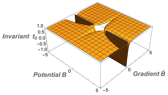
In principle, this expression can be reduced to quadratures. However, the form of the left-hand-side makes this analytically unfeasible in practice and one has to resort to numerical techniques. Nonetheless, one can perform a qualitative analysis of the behaviour of solutions to (19) by plotting level curves defined by the invariant (20). Plots of (20) are given in Figure 1 (), Figure 2 () and Figure 3 (). We also present the plots for and in Figure 4 so that the behaviour of solutions to (19) can be compared across dimensions. The latter forms an envelope as depicted in Figure 5.
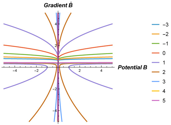
Figure 1.
Level curves for (20) with and . Each curve corresponds to different values of the invariant as indicated in the legend.
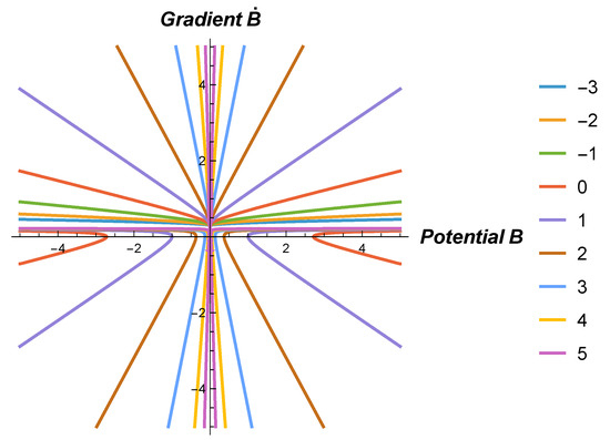
Figure 2.
Level curves for (20) with and . Each curve corresponds to different values of the invariant as indicated in the legend.
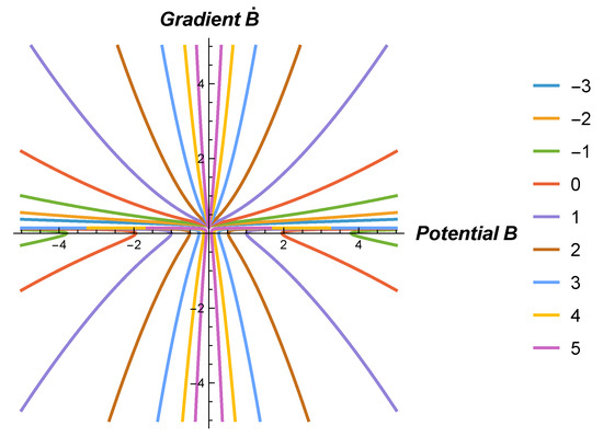
Figure 3.
Level curves for (20) with and . Each curve corresponds to different values of the invariant as indicated in the legend.
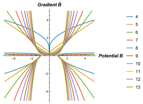
Figure 4.
Level curves for (20) with . Each curve corresponds to different values of dimension N as indicated in the legend.
3.1.3. Nonlinear
Nonlinear forms of may solve (13). By attempting different forms of , we were guided to the representation
For consistency we must have that and and
while
must hold. Note, though, that a is a free parameter. Thus, the nonlinear metric potential function
satisfies the boundary condition (13). The potential in (23) is a new result in higher dimensions N. The spacetime dimension N affects the magnitude of the gravitational potential.
Invoking the translational invariance of (13) again, we can write the two-parameter solution of (13), subject to (22), as
where both a and are free parameters. We emphasise that the expression in (24) contains two constants a and , meaning that it is a general solution of (13) subject to (22).
It is also important to note that the general solution (24) is not contained in handbooks of solutions to differential equations; software packages such as Mathematica and Maple do not give this exact solution. The exact solution
obtained by Paliathanasis et al. [35] arises as a special case of (24) (equivalently (23)) when and In summary, the spacetime dimension N changes the form of the potential and therefore influences the evolution of the radiating star.
3.1.4.
The final case we consider is that of . We do not consider as this would force to be zero and, therefore, the metric potential A would be a constant. If vanishes at the boundary, one of the free parameters in (12) is constrained, e.g.,
Now we merely have to analyse
which is a homogeneous equation in .
We note that (27) admits the linear solution (16) with
but this is the only power law solution to (27), i.e., solutions of the form (23) do not exist.
Observe that (27) can be reduced to the quadrature
where and are arbitrary parameters (integration constants). This integral can be evaluated, in general, in terms of the hypergeometric function , viz.
which simplifies in special cases. In particular, when , we obtain the implicit solution
given in terms of logarithms. When , we obtain the explicit solution
given in terms of special functions, namely the Lambert W function [42]. For odd , we obtain implicit solutions in terms of inverse tangent functions and other elementary functions. For example, for we obtain
with logarithms and trigonometric functions arising for odd . For even , the hypergeometric solutions do not simplify further. Note that, in the solutions presented above, the arbitrary parameters have often been redefined for simplicity.
However, the behaviour of the solutions of (27) is more readily understood by looking at its phase portrait via the system
This system possesses a continuous line of fixed points at . These fixed points are stable when and unstable when corresponding to stable and unstable half-lines. Thus, one can obtain a stellar configuration which culminates in a static state (in the former case) or starts from an initial static state and then radiates (in the latter case)—see Figure 6 and Figure 7. In this analysis, the dimension N does not affect the asymptotic behaviour of the solutions of (27). However, we note that there exists a nullcline at . Thus, the described behaviour only occurs when for or for again corresponding to stable and unstable half-lines. In particular, this restricts the basin of attraction for the stable half-line. Outside this region, solutions either approach zero asymptotically or blow up. We note that and so the nullcline coincides with the continuous line of fixed points in the limit.
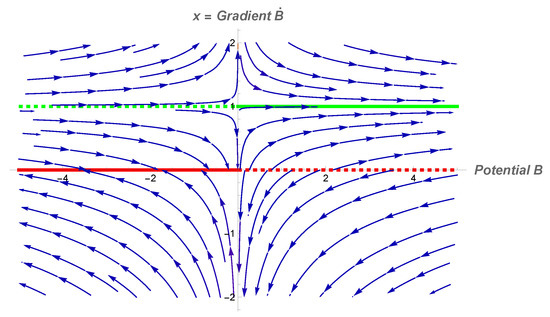
Figure 6.
Phase diagram for (27) with and . The red line denotes the continuous line of fixed points with the solid half-line indicating the set of stable fixed points while the dashed half-line indicates the set of unstable fixed points. The solution is undefined along . The nullcline is indicated in green with the solid portion indicating the attracting half-line while the dashed portion indicates the repelling half-line.
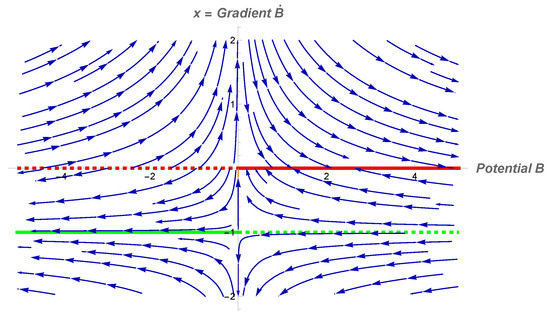
Figure 7.
Phase diagram for (27) with and . The red line denotes the continuous line of fixed points with the solid half-line indicating the set of stable fixed points while the dashed half-line indicates the set of unstable fixed points. The solution is undefined along . The nullcline is indicated in green with the solid portion indicating the attracting half-line while the dashed portion indicates the repelling half-line.
This analysis shows the interesting physical features of the asymptotic temporal behaviour of the radiating star without specifying the gravitational potential . The star approaches an asymptotic static configuration or continues to radiate. Govender et al. [43] generated a radiating model undergoing gravitational collapse, leading to a static configuration representing a superdense star. Most other models that have been found continue to radiate as in the treatments of Chan [44] and Pinheiro and Chan [45]. Our analysis provides a qualitative basis for the existence of both sets of solutions.
3.2. Unconstrained Solutions
While Equation (13) is a nonlinear equation, progress can still be made. We observe that (13) is invariant under both scaling and translational transformations. This means that it can be reduced to quadratures. We achieve this reduction by first determining a first integral. We let and . Then (13) can be written as
which is a special case of Chini’s differential equation [46]. The Chini equation also arises in the study of static charged gravitating spheres in Einstein–Gauss–Bonnet gravity [47]. Further to this, Equation (35) is separable in y and x and thus, after some calculation (and inverting our transformation), the solution can be written in the form
which can be simplified to
where and are (related) integration constants. The expression (36) is a first integral of (13) in higher dimensions. It contains the limiting case of .
Note that , as given in (17), must be non-zero. The case of vanishing was analysed separately earlier.
In principle, (36) can be solved for , and the resulting equation will be of variable separable form and so directly integrated. In practice though, this inversion is unfeasible and so we make recourse to qualitative methods.
3.3. Asymptotic Analysis
A qualitative view of the behaviour of unconstrained solutions to (13) can be obtained via a phase plane analysis. However, since (13) does not admit any constant solutions in general, no fixed points exist. Fortunately, the first integral (36) can be found explicitly and so we can undertake a phase plane analysis. This expression defines level curves on an invariant sub-manifold. Plotting these curves will provide a holistic view of the behaviour of the system, without being constrained by particular solutions.
A direct way to proceed is to simply treat (36) as a function of and B and plot this function. In order to do this, we set
and then .
In Figure 8 we present plots of versus B for different values of N. Each pair of symmetric curves represents a different dimension. The behaviour is consistent across dimensions and for different values of the first integral. This can be seen in Figure 9 (), Figure 10 () and Figure 11 (). Figure 9 is of particular importance as, in a previous study [40], the singularity at prevented a standard phase plane analysis for .
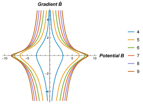
Figure 8.
Level curves using the first integral (36) with . Each symmetric pair of curves represents a different dimension N as indicated in the legend.
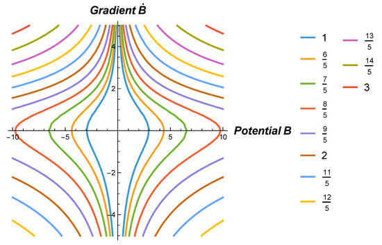
Figure 9.
Level curves using the first integral (36) with . Each symmetric pair of curves represents a different value of as indicated in the legend.
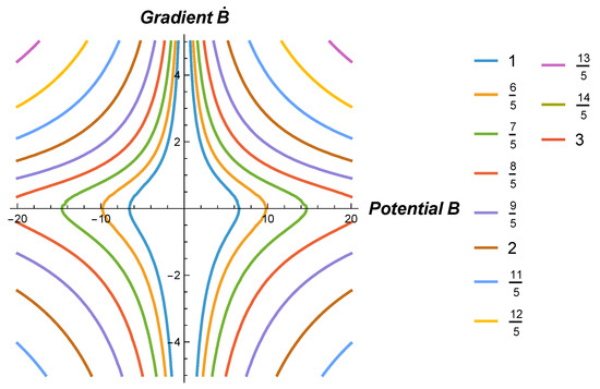
Figure 10.
Level curves using the first integral (36) with . Each symmetric pair of curves represents a different value of as indicated in the legend.
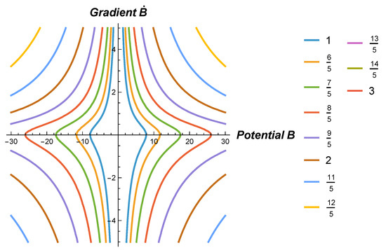
Figure 11.
Level curves using the first integral (36) with . Each symmetric pair of curves represents a different value of as indicated in the legend.
4. Luminosity and Physical Features
One important physical property of a radiating star is the notion of horizon formation. In the scenario where the rate of a collapsing sphere dissipating energy in the form of a radial heat flux is balanced by the rate of emission of energy, the horizon may not form—this was shown for the linear solution in the four-dimensional case, i.e., is independent of time [30]. The other physically important quantity is the luminosity. The luminosity observed by an observer positioned at infinity from the radiating star is given by
where the matching conditions for the smooth matching of the line element (1) and the higher-dimensional analogue of Vaidya’s outgoing solution (5) give us
where is the proper time measured by a comoving observer on the timelike hypersurface forming the boundary between the interior and exterior spacetimes. The continuity of the first and second fundamental forms, which ensure the smooth matching of the interior and exterior spacetimes, yields the following for the higher-dimensional mass function [48]:
which was first derived in [31]. For the linear solution (14), the luminosity at infinity takes the form
We note that, in four dimensions, the luminosity is independent of time as observed by Banerjee et al. [30]. The following question then arises: what is the end state of this collapse scenario for ? The time of formation of the horizon is obtained when , implying that an observer located at infinity will observe an infinite redshift of the emitted radiation. The magnitude of the luminosity grows with increasing dimension and is simultaneously strengthened by the temporal evolution for . For all collapse scenarios , the luminosity vanishes as since . For the assumption (10), takes the form
Substituting the power-law solution (23) into (42) and requiring it to vanish, we find that the time of formation of the horizon is sensitive to the ratio and the horizon forms earlier compared to the linear case.
In Figure 12, it is clear for this epoch that the density is well behaved, attaining a maximum value at the centre of the stellar configuration and dropping monotonically towards the boundary. As the collapse proceeds, we observe that the density increases as expected since the star is collapsing, and in the process, matter is squeezed into smaller volumes. It is interesting to note the effect of spacetime dimension on the stellar density. As the dimension increases, there is a corresponding increase in density. For example, the increase in density for a star in four-dimensional spacetime to a star in ten-dimensional spacetime is approximately 96%. The increase in spacetime dimensionality has the effect of squeezing more matter into smaller concentric shells surrounding the stellar centre.
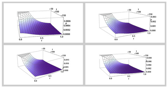
Figure 12.
The above figures show the behaviour of the density as a function of the radial and temporal coordinates with varying dimensionality, starting with in the top left figure, and moving clockwise to , and finally , bottom left.
From Figure 13, we note that the pressure decreases smoothly towards the surface layers of the star. As the collapse proceeds, the pressure increases dramatically due to increased heating and energy generation within the core. As with the density, we observe that an increase in spacetime dimensionality results in an increase in the magnitude of p with the increase being most significant in regions closer to the centre. When N increases from to , this results in an increase in pressure of the order of . It is clear that spacetime dimensionality significantly affects the thermodynamical properties of the star.
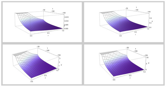
Figure 13.
The behaviour of the pressure profiles as a function of the radial and temporal coordinates with varying dimensionality are displayed in this panel, starting with in the top left figure, and moving clockwise to , and finally , bottom left.
We have also plotted the luminosity profile for in Figure 14. We observe that the luminosity is a decreasing function of t and vanishes at . For the case , the luminosity is constant and the horizon never forms. For a fixed set of parameter values, , the luminosity at infinity evolves as , and for , and , respectively, where s are constants. Our model shows that luminosity as observed by an observer placed at infinity increases with spacetime dimension.
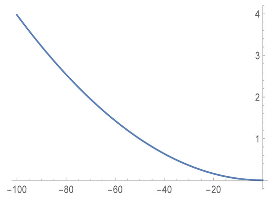
Figure 14.
Luminosity profile as a function of the temporal coordinate for .
In addition, we observe the following salient features of our model which holds true for different dimensions: , , , and . Since the star is dissipating energy, the additional condition is obeyed, and (where ) throughout the stellar interior [30].
5. Discussion
We have performed a detailed analysis of a radiating star in general relativity in higher dimensions. To study the temporal behaviour of the star, we have selected a separable form of the metric functions in a shear-free matter distribution. Exact solutions to the boundary condition were found that govern the evolution of the star in higher spacetime dimensions . When , we regain the models of Banerjee et al. [30,31] and Paliathanasis et al. [35]. When , the gravitational potential depends explicitly on the spacetime dimension. Therefore, the parameter N influences the temporal evolution of the star and affects the magnitude of the potentials. First integrals for the boundary condition can be found which contain the potential and its derivative . The behaviour of the gravitational potential can then be determined numerically. A phase plane analysis of the boundary condition was undertaken. The result of this investigation shows that the radiating star approaches a static asymptotic end state or the star continues to radiate from an initially static configuration. Consequently, the phase plane analysis reveals interesting physical features of the asymptotic behaviour in the temporal evolution of the radiating star. It is important to note that the phase plane treatment does not require a specific choice of the potential ; the results obtained will hold in general for the shear-free metrics (1) with . It would be interesting to extend our approach to shearing metrics, which is an area of future study. The dimensionality of the manifold changes the physical features of the radiating model. We show, in particular, that there is a change in luminosity in higher dimensions.
Author Contributions
Conceptualisation, S.D.M., B.P.B., M.G. and K.S.G.; methodology, S.D.M., B.P.B., M.G. and K.S.G.; software, K.S.G.; validation, S.D.M., B.P.B., M.G. and K.S.G.; formal analysis, S.D.M., B.P.B., M.G. and K.S.G.; original draft preparation, S.D.M., B.P.B., M.G. and K.S.G.; writing—review and editing, S.D.M., B.P.B., M.G. and K.S.G. All authors have read and agreed to the published version of the manuscript.
Funding
S.D.M. and K.S.G. thank the University of KwaZulu–Natal for ongoing support. M.G. acknowledges financial support from the National Research Foundation under grant number 146050.
Data Availability Statement
All data that support the findings of this study are included in the article.
Conflicts of Interest
The authors declare no conflicts of interest.
References
- Paul, B.C. On the mass of a uniform density star in higher dimensions. Class. Quantum Grav. 2001, 18, 2637. [Google Scholar] [CrossRef]
- Chattopadhyay, P.K.; Deb, R.; Paul, B.C. Relativistic charged star solutions in higher dimensions. Int. J. Theor. Phys. 2014, 53, 1666–1684. [Google Scholar] [CrossRef]
- Arbanil, J.D.V.; Lenzi, C.H.; Malheiro, M. Fluid pulsation modes from strange stars in a higher-dimensional spacetime. Phys. Rev. D 2020, 102, 084014. [Google Scholar] [CrossRef]
- Saha, A.; Goswami, K.B.; Das, B.; Chattopadhyay, P.K. Maximum mass of anisotropic charged strange quark stars in a higher dimensional approach (D ≥ 4). Chin. Phys. C 2023, 47, 015107. [Google Scholar] [CrossRef]
- Paul, B.C. Relativistic star solutions in higher dimensions. Int. J. Mod. Phys. D 2004, 13, 229–238. [Google Scholar] [CrossRef]
- Khadekov, G.S.; Warjari, R. Geometry of quark and strange quark matter in higher dimensional general relativity. Int. J. Theor. Phys. 2012, 51, 1408–1415. [Google Scholar] [CrossRef]
- Goswami, K.B.; Roy, R.; Saha, A.; Chattopadhyay, P.K. Strange Quark Star (SQS) in Tolman IV potential with density dependent B-parameter and charge. Eur. Phys. J. C 2022, 82, 1042. [Google Scholar] [CrossRef]
- Chattopadhyay, P.K.; Paul, B.C. Relativistic star solutions in higher-dimensional pseudospheroidal space-time. Pramana 2010, 74, 513–523. [Google Scholar] [CrossRef]
- Paul, B.C.; Chattopadhyay, P.K.; Karmarkar, S. Relativistic anisotropic star and its maximum mass in higher dimensions. Astrophys. Space Sci. 2015, 356, 327–337. [Google Scholar] [CrossRef]
- Saha, A.; Goswami, K.B.; Chattopadhyay, P.K. Anisotropic star in Vaidya-Tikekar model admitting MIT bag model equation of state in pseudo-spheroidal geometry. Astrophys. Space Sci. 2021, 366, 98. [Google Scholar] [CrossRef]
- Goswami, K.B.; Chattopadhyay, P.K. New class of relativistic anisotropic strange star in Vaidya-Tikekar model. Astrophys. Space Sci. 2020, 365, 141. [Google Scholar] [CrossRef]
- Dey, S.; Paul, B.C. Higher dimensional charged compact objects in Finch–Skea geometry. Class. Quantum Grav. 2020, 37, 075017. [Google Scholar] [CrossRef]
- Hendi, S.H.; Bordhar, G.H.; Eslam Panah, B.; Panahiyan, S. Modified TOV in gravity’s rainbow: Properties of neutron stars and dynamical stability conditions. J. Cosmol. Astropart. Phys. 2016, 09, 013. [Google Scholar] [CrossRef]
- Das, B.; Dey, S.; Das, S.; Paul, B.C. Anisotropic compact objects with Finch–Skea geometry in EGB gravity. Eur. Phys. J. C 2022, 82, 519. [Google Scholar] [CrossRef]
- Zubair, M.; Farooq, M.; Bhar, P.; Azmat, H. Modelling of stellar solutions in Einstein-Gauss-Bonnet gravity. Chin. J. Phys. 2024, 88, 129–145. [Google Scholar] [CrossRef]
- Karmakar, A.; Debnath, U.; Deb, R. Polytropic stellar structure in 5D Einstein-Gauss-Bonnet gravity. Chin. J. Phys. 2024, 90, 1125–1142. [Google Scholar] [CrossRef]
- Karmakar, A.; Rej, P.; Salti, M.; Oydogdu, O. Charged quark stars represented by the MIT bag approach in 5D Einstein-Maxwell-Gauss-Bonnet gravity formalism. Eur. Phys. J. Plus 2023, 138, 914. [Google Scholar] [CrossRef]
- Karmakar, A.; Rej, P. Celestial attributes of hybrid star in Einstein-Gauss-Bonnet gravity. Chin. J. Phys. 2024, 87, 155–173. [Google Scholar] [CrossRef]
- Gumede, S.C.; Maharaj, S.D.; Govinder, K.S. The role of dimensions in gravitating relativistic shear-free fluids. Eur. Phys. J. C 2024, 84, 862. [Google Scholar] [CrossRef]
- Pinheiro, G.; Chan, R. Radiating gravitational collapse with shear viscosity. Gen. Relativ. Gravit. 2008, 40, 2149–2175. [Google Scholar] [CrossRef]
- Tewari, B.C. Relativistic collapsing radiating stars. Astrophys. Space Sci. 2012, 342, 73–77. [Google Scholar] [CrossRef]
- Tewari, B.C. Collapsing shear-free radiating fluid spheres. Gen. Relativ. Gravit. 2013, 45, 1547–1558. [Google Scholar] [CrossRef]
- Charan, K.; Yadav, O.P.; Tewari, B.C. Charged anisotropic spherical collapse with heat flow. Eur. Phys. J. C 2021, 81, 60. [Google Scholar] [CrossRef]
- Jaryal, S.C. Radiating-collapsing models satisfying Karmarkar condition. Eur. Phys. J. C 2020, 80, 683. [Google Scholar] [CrossRef]
- Ospino, J.; Nunez, L.A. Karmarkar scalar condition. Eur. Phys. J. C 2020, 80, 166. [Google Scholar] [CrossRef]
- Santos, N.O. Non-adiabatic radiating collapse. Mon. Not. R. Ast. Soc. 1985, 216, 403–410. [Google Scholar] [CrossRef]
- Maharaj, S.D.; Brassel, B.P. Radiating stars with composite matter distributions. Eur. Phys. J. C 2021, 81, 366. [Google Scholar] [CrossRef]
- Maharaj, S.D.; Brassel, B.P. Junction conditions for composite matter in higher dimensions. Class. Quantum Grav. 2021, 38, 195006. [Google Scholar] [CrossRef]
- Bhui, B.; Chatterjee, S.; Banerjee, A. Non-adiabatic gravitational collapse in higher dimensional space-time and its junctions conditions. Astrophys. Space Sci. 1995, 226, 7–18. [Google Scholar] [CrossRef]
- Banerjee, A.; Chatterjee, S.; Dadhich, N. Spherical collapse with heat flow and without horizon. Mod. Phys. Lett. A 2002, 17, 2335–2339. [Google Scholar] [CrossRef]
- Banerjee, A.; Chatterjee, S. Spherical collapse of a heat conducting fluid in higher dimensions without horizon. Astrophys. Space Sci. 2005, 299, 219–225. [Google Scholar] [CrossRef]
- Shah, H.; Ahmed, Z.; Khan, S. Higher dimensional shear-free radiating collapse. Can. J. Phys. 2018, 96, 1201–1204. [Google Scholar] [CrossRef]
- Khan, S.; Habib, F.; Shah, H.; Alkhaldi, A.H.; Ali, A. Higher dimensional collapsing and expanding models of anisotropic source. Results Phys. 2021, 29, 104712. [Google Scholar] [CrossRef]
- Feng, W.X. On the dynamical instability of monatomic fluid spheres in (N + 1)-dimensional spacetime. Astronomy 2023, 2, 22–46. [Google Scholar] [CrossRef]
- Paliathanasis, A.; Govender, M.; Leon, G. Temporal evolution of a radiating star via Lie symmetries. Eur. Phys. J. C 2021, 81, 718. [Google Scholar] [CrossRef]
- Leon, G.; Govender, M.; Paliathanasis, A. Lie symmetries, Painlevé analysis, and global dynamics for the temporal equation of radiating stars. Math. Methods Appl. Sci. 2022, 45, 7728–7743. [Google Scholar] [CrossRef]
- Chan, R. A shearing Non-adiabatic solution of Einstein’s equations. Astrophys. Space Sci. 1997, 257, 299–309. [Google Scholar] [CrossRef]
- Tewari, B.C. Relativistic Model for Radiating Star. Astrophys. Space Sci. 2006, 306, 273–277. [Google Scholar] [CrossRef]
- Das, S.; Sharma, R.; Paul, B.C.; Deb, R. Dissipative gravitational collapse of an (an)isotropic star. Astrophys. Space Sci. 2016, 361, 99. [Google Scholar] [CrossRef]
- Maharaj, S.D.; Govinder, K.S. Dynamics of the temporal evolution in radiating stars. Gen. Relativ. Gravit. 2025, 57, 11. [Google Scholar] [CrossRef]
- Banerjee, A.; Dutta Choudhury, S.B.; Bhui, B.K. Conformally flat solution with heat flux. Phys. Rev. D 1989, 40, 670. [Google Scholar] [CrossRef]
- Corless, R.M.; Gonnet, G.H.; Hare, D.E.G.; Jeffrey, D.J.; Knuth, D.E. On the Lambert W function. Adv. Comput. Math. 1996, 5, 329–359. [Google Scholar] [CrossRef]
- Govender, M.; Govinder, K.S.; Maharaj, S.D.; Sharma, R.; Mukherjee, S.; Dey, T.K. Radiating spherical collapse with heat flow. Int. J. Mod. Phys. D 2003, 12, 667–676. [Google Scholar] [CrossRef]
- Chan, R. Radiating gravitational collapse with shear revisited. Int. J. Mod. Phys. D 2003, 12, 1131–1155. [Google Scholar] [CrossRef]
- Pinheiro, G.; Chan, R. Radiating gravitational collapse with shearing motion and bulk viscosity revisited. Int. J. Mod. Phys. D 2010, 19, 1797–1822. [Google Scholar] [CrossRef]
- Chini, M. Sull’integrazione di alcune equazioni differenziali del primo ordine. Rend. Inst. Lomb. 1924, 57, 506. [Google Scholar]
- Ismail, M.O.E.; Maharaj, S.D.; Brassel, B.P. The Chini integrability condition in second order Lovelock gravity. Eur. Phys. J. C 2024, 84, 1330. [Google Scholar] [CrossRef]
- Goswami, R.; Joshi, P.S. Spherical gravitational collapse in N dimensions. Phys. Rev. D 2007, 76, 084026. [Google Scholar] [CrossRef]


Disclaimer/Publisher’s Note: The statements, opinions and data contained in all publications are solely those of the individual author(s) and contributor(s) and not of MDPI and/or the editor(s). MDPI and/or the editor(s) disclaim responsibility for any injury to people or property resulting from any ideas, methods, instructions or products referred to in the content. |
© 2025 by the authors. Licensee MDPI, Basel, Switzerland. This article is an open access article distributed under the terms and conditions of the Creative Commons Attribution (CC BY) license (https://creativecommons.org/licenses/by/4.0/).