Abstract
When a CME arrives at the Earth, it will interact with the magnetosphere, sometimes causing hazardous space weather events. Thus, the study of CMEs which arrived at Earth (hereinafter, Earth-impacting CMEs) has attracted much attention in the space weather and space physics communities. Previous results have suggested that the three-dimensional parameters of CMEs play a crucial role in deciding whether and when they reach Earth. In this work, we use observations from the Solar TErrestrial RElations Observatory (STEREO) to study the three-dimensional parameters of 71 Earth-impacting CMEs from the middle of 2008 to the end of 2012. We find that the majority Earth-impacting CMEs originate from the region of [30S,30N] × [40E,40W] on the solar disk; Earth-impacting CMEs are more likely to have a central propagation angle (CPA) no larger than half-angular width, a negative correlation between velocity and acceleration, and propagation time is inversely related to velocity. Based on our findings, we develop an empirical statistical model to forecast the arrival time of the Earth-impacting CME. Also included is a comparison between our model and the aerodynamic drag model.
1. Introduction
A Coronal Mass Ejection (CME) is a powerful solar explosion that contains a huge amount of plasma with energy of ∼ erg and mass of ∼ g [1,2,3]. The interplanetary counterpart of the CME is called the Interplanetary Coronal Mass Ejection (ICME).
The properties of ICMEs can be analyzed by in-situ observations using spacecraft such as WIND [4]. Previous studies have shown that ICMEs often contain some or all of the following observational features: (1) enhanced magnetic field strength [5]; (2) large and smooth magnetic field rotation [5]; (3) gradually decreasing solar wind speed [5]; (4) lower proton temperature [6]; (5) lower plasma [7]; (6) obvious bidirectional electron streaming [8]; (7) abnormal charge state of ions [9,10]; and (8) abnormal particle abundance [11,12]. According to whether the characteristics (1), (2), (5) are strictly met, ICMEs can be divided into magnetic clouds (MCs) and non-MCs [13]. Based on these criteria, some ICME catalogs have been established, and various statistical studies have been carried out for a more comprehensive understanding of ICMEs [14,15,16]. The ICMEs may interact with the Earth’s magnetosphere and cause some hazardous space weather events, such as intense geomagnetic storms [17,18]. Hence, it’s of great significance to study such events. Since these ICMEs’ properties are mainly obtained from in-situ observations close to the Earth, we can only provide an average warning time of one hour before the ICME hits the Earth, which is far from enough. On the other hand, the initial properties of CMEs obtained from the coronagraph observations could serve as early signals of whether and when the CME will reach the Earth, giving us ample time to mitigate the impact of severe space weather events.
According to the literature, the daily CME rate averaged over one Carrington Rotation period increases from one every two days during solar minimum to more than six per day during solar maximum [19,20]. However, owing to the different propagation directions and the influence of Interplanetary Magnetic Field (IMF), not all CMEs eventually arrive in the vicinity of Earth, i.e., not all the CMEs are Earth-impacting CMEs. So some questions come up naturally: what kind of CMEs can arrive at the Earth and when will such CMEs arrive? Previous results suggest that the three-dimensional parameters of CMEs, such as source location [21,22,23,24,25,26,27,28], angular width [22,28,29], and propagation angle [22,28,29] as well as the initial velocity [21,22,24,25,26,27,28,29,30,31], are important factors in determining whether and when they arrive at Earth.
Although authors are aware of the importance of CME’s three-dimensional parameters, due to the limitations of observational instruments, many CMEs studies [26,32,33] are mainly conducted using a single spacecraft (single observation angle). For example, Wang et al. (2002) [26] did a statistical study on the geoeffectiveness of Earth-directed coronal mass ejections from March 1997 to December 2000 based on the observations of the Large Angle Spectroscopic COronagraph (LASCO) [34] and Extreme ultraviolet Imaging Telescope (EIT) [35] onboard SOlar and Heliospheric Observatory (SOHO) [36]. Their results suggest that the initial sites of the frontside halo CMEs are around in latitude and the CMEs transit time show a weak correlation with the CME projected speed. These conclusions have been verified by some other works [27,29].
Multi-spacecraft observations of CMEs have been available since the launch of the Solar TErrestrial RElations Observatory (STEREO) [37] on 26 October 2006, thanks to STEREO Ahead (A) and Behind (B; lost signal October 2014)’s dynamic separation angle, which allows the coronagraph onboard these two spacecraft to observe the solar atmosphere from two different perspectives. The possible projection effect from single perspective observation can be significantly reduced. Based on the observational data from STEREO, many three-dimensional CME models were developed, such as Graduated Cylindrical Shell (GCS) [38,39,40], triangulation methods [41,42,43,44], mask fitting methods [45], Geometric Localization [46], Local Correlation Tracking Plus Triangulation [47]. Lugaz et al. (2010) [48] and Feng et al. (2013) [49] discussed the accuracy and the differences of some models, with the help of those models the geometric parameters of CMEs could be more reliably studied and analyzed.
Among these models, the GCS model is one of the most widely used forward models. For example, Shen et al. (2014) [28] used GCS model fitting to obtain the geometric parameters of frontside full-halo CMEs (FFHCMEs) from 16 December 2009 to 17 May 2012. Their analysis suggest that central CMEs, which propagate in the longitude range [E, W] or with deviation angle no larger than have a higher probability of arriving at the Earth; and FFHCMEs with an angular width of more than twice the deviation angle can hit the Earth, which may become a useful simple criterion to forecast whether a CME is Earth-impacting. Their work also suggest that the self-similar expansion model combined with the aerodynamic model [50] is a simple and useful tool to forecast the arrival time of CME. Shi et al. (2015) [31] also used the GCS model to get the initial speeds for 21 CMEs during 2008–2012 and predicted the arrival time of CMEs to the Earth. Their result provide a method of forecasting space weather 1–5 days following the occurrence of CMEs with fairly good accuracy.
A CME that could be found in the associated frontside solar event is considered to be frontside or Earth-directed, while a halo CME is thought to have an apparent size greater than 130 [26]. Hence, to study what kind of CMEs are Earth-impacting, Earth-directed or frontside halo CMEs are obviously of interest. Many studies on Earth-impacting CMEs or geoeffective CMEs have focused on such CMEs [21,23,25,26,28,30]; however, sometimes an Earth-impacting CME is not necessarily a halo. Therefore, there are some studies [24] that analyze the characteristics of Earth-impacting or geoeffective CMEs and obtain some necessary but not sufficient conditions for Earth-impacting CME forecasting.
In this work, the three-dimensional parameters of all Earth-impacting CMEs recorded by STEREO and SOHO (2008–2012) are obtained through the GCS model. Then, we conduct some statistical analysis, trying to find the common features of these Earth-impacting CMEs, and compare our findings to previous studies to obtain a better and fuller picture of Earth-impacting CMEs. This paper is organized as follows: in Section 2, we present a simple explanation of the events we studied, as well as a brief introduction to the GCS model; the fitting results are shown in Section 3; in Section 4, we show how the results are processed and analyzed; finally, we give a conclusion and discussion in Section 5.
2. Data Collection & Method of Fitting
In recent work, Chi et al. (2016) [16] established a new online ICME catalog (http://space.ustc.edu.cn/dreams/wind_icmes/ (accessed on 23 July 2021)), mainly based on the WIND magnetic field and plasma observations from 1996 to 2014. In our work, to obtain Earth-impacting CMEs, as with a similar method illustrated in Chi et al. (2018) [51], we first check in-situ observations from this catalog to obtain information about ICMEs including their start time and average speed. According to this information about ICMEs, we deduce the possible eruption time of the progenitor solar CMEs. Then we search for a corresponding CME observation using J-map [52] with a 10 day long continuous window. Next, we check the STEREO-COR2 (https://stereo-ssc.nascom.nasa.gov/data.shtml (accessed on 23 July 2021)) observed images to find the corresponding CMEs. If the corresponding CMEs are found, we confirm the information about these CMEs in the observation of SOHO by combining the CME list of CDAW (Coordinated Data Analysis Workshop: http://cdaw.gsfc.nasa.gov/CME_list/ (accessed on 23 July 2021)). Note that, if there are multiple alternative CMEs, especially during times of higher solar activity, we use the GCS model to obtain the velocities and directions of all these CMEs and pick out the most likely progenitor CME. Finally, we obtain an ICME–CME list (see Appendix A.1 Table A1) which contains a series of Earth-impacting CMEs from 21 July 2008 to 11 December 2012. A total of 91 ICMEs have been observed during this period, with the solar source of 77 of those ICMEs being more certain. As a result, these 77 ICMEs will be analyzed in this paper.
The data we use are the white-light coronographic observations from the LASCO instrument onboard SOHO and the Sun-Earth-Connection Coronal and Heliospheric Investigation (SECCHI) [53] onboard STEREO [37].
The model we use to obtain the three-dimensional parameters of the Earth-impacting CMEs is the GCS model. This model is a kind of empirical model meant to reproduce the large-scale structure of flux-rope-like CMEs [38,39,40], which consist of a tubular section forming the main body of the structure attached to two cones that correspond to the “legs” of the CME. It expands in a self-similar way. According to the mathematical deduction from Thernisien (2011) [40], the GCS model has six free geometric parameters, including the longitude (), latitude (), tilt angle (), the height of the CME’s leading edge (), the half-angle of one cone () and the half-angle between the axis of two cones ().
After selecting the events, we use the GCS model based on (IDL) and (SSW) to obtain these six geometric parameters of the CMEs mentioned above. To be specific, we need to obtain the maximum similarity between the projections of the GCS model (the green wireframe in Figure 1d–f) and the actual observations of the white-light coronagraph of CMEs (images like Figure 1a–c) by adjusting the six parameters of the flux rope manually, that is, the forward fitting method. After fitting, we can obtain the GCS model’s six geometric parameters of each CME event in a time series during its evolution in the field-of-view of three coronagraphs.
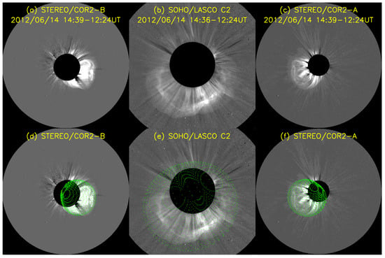
Figure 1.
The GCS model fitting result of Earth-impacting CME occurred at 14 June 2012. (a–c) the base-difference imaging observations of this CME by (from left to right) STEREO-A, SOHO-LASCO-C2 and STEREO-B, respectively. (d–f) the fitted GCS model is overlaid as the green wire frame.
Before using these parameters to do any analysis, we have performed some simple processing of them. First, the actual half-angular width equals the half-angular width between two cone axis plus half-angular width of one cone (hereinafter, we use to represent the half-angular width), which means that (). Then, we do the linear fitting for the time series of to get the average initial velocity () of CMEs. At last, we do the quadratic polynomial fitting for the time series of again and got the initial acceleration () of CMEs. An example of these two kinds of fitting results is presented in Figure 2. This CME event occurred on 6 June 2012.
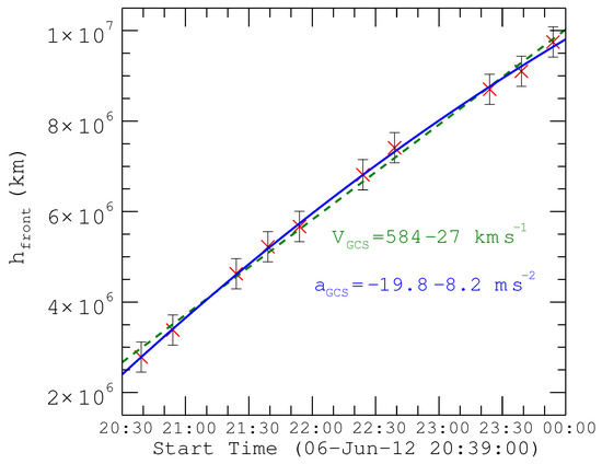
Figure 2.
Linear fitting and quadratic polynomial fitting results for the time series of of the event on 6 June 2012.
In Figure 2, the red cross symbols (x) mark the actual measure of , the green dash line is the linear fitting result and the texts with the same color are the linear velocity we obtain, the blue line and the acceleration information in texts of the same color are the results from quadratic polynomial fitting.
3. Results
In Section 2, we mention that there are 77 Earth-impacting CMEs that can be used for the analysis. After finishing GCS fitting and some early simple data processing, we find that eight CMEs among the 77 events are not suitable to be modeled by the GCS model and should be excluded. We suspect that two special events (ICME around 07:30:00 UT, 21 June 2010 and 05:33:00 UT, 28 May 2011 [51]) are the results of two CMEs’ interaction, thus we perform GCS fitting for both of the two source CMEs. That means that we finally obtain 71 sets of fitting results. These three-dimensional parameters and some other useful information about the Earth-impacting CMEs are listed in Table 1. Columns from left to right are the sequence number of the CME (No.), initial fitting time (Time_fit), longitude (, positive for west), latitude (, positive for north), tilt angle (), half-angular width (), the average initial velocity (), the initial acceleration () and the time for the start of the ejecta (Time_arrive) observed by WIND, respectively. Note that we only list the initial value of , and for each event due to the possible deflection by Parker spiral magnetic field [27] after that time.

Table 1.
The GCS’ Fitting Results of CMEs.
The uncertainties come from the errors of the original six parameters in the GCS model fitting process. A study by Thernisien et al. (2009) [39] shows the mean uncertainties in the GCS model are about , , , , and R (solar radii) for , , , , and , respectively. Our analysis will use these uncertainties as a reference. So, the uncertainty of can be derived, which is about . By taking the uncertainty of into the linear fitting and the quadratic polynomial fitting process, the uncertainties of and for each event can also be calculated. The uncertainties of and are shown in Table 1.
Now we have the parameters of CME’s longitude, latitude, tilt angle, half-angular width, velocity and acceleration. Next, we will analyze the characteristics of these Earth-impacting CMEs, as shown in the following section.
4. Analysis of Various Properties of Earth-Impacting CMEs
4.1. Location
The first concern in predicting Earth-impacting CME is whether there is a CME, specifically we need to know the explosion time and locations of CMEs. However, due to the obscure physical mechanism of CMEs, it is hard to know these two pieces of information in advance by theoretical derivation. So what we can do now is just giving an early warning based on the observation of ongoing CMEs. In this subsection, the locations and other location-related properties of Earth-impacting CMEs are discussed using data from Table 1.
To get a general view of the locations of these Earth-impacting CMEs, we mark them on solar disk like Figure 3. On the top panel, red diamond symbols stand for CMEs appeared on the solar disk (observed from the Earth, the same goes for later descriptions). The bottom panel of Figure 3 shows a scatter graph of and with red diamond symbols. The two horizontal dashed blue lines mark the maximum and minimum values of , which are 43.00 and −30.18, respectively. The enclosed region between two vertical blue dashed lines stands for the front-side solar disk ( between −90 and 90 degrees).
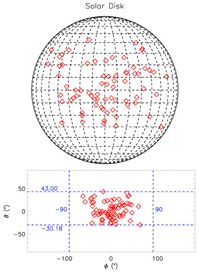
Figure 3.
Locations of CMEs on Solar Disk (top) and Rectangular Coordinate System of Longitude-Latitude (bottom).
If we focus on the latitudinal information, Figure 3 reveals that Earth-impacting CMEs are concentrated in the region between 30 north and 30 south, with specific value (about ). As for longitude, Cane et al. [54] suggested that the location of typical Earth-impacting solar events are in longitude ≤40 east and west. In this work, (about ) of CMEs locate at longitude of ∼, and more than half (, ∼55%) of CMEs come from ∼. The easternmost and westernmost longitudinal locations are and , respectively, which shows the possibility that some Earth-impacting CMEs originate far from the central region.
According to the characteristic of latitudinal and longitudinal distribution of these Earth-impacting CMEs, we suggest that all the Earth-impacting CMEs are distributed at the front of the solar disk, and are concentrated near the central region except fairly few of them are scattered toward to the solar limb. Given that all these CMEs are Earth-impacting, it seems that deflections of these CMEs beyond the field of view of STEREO/COR2 and LASCO/C2 are not significant. Based on this conclusion, we assume that most Earth-impacting CMEs move outward almost in a radial direction for further analysis in Section 4.2 and Section 4.3.
4.2. Central Propagation Angle & Half-Angular Width
After obtaining the locations of Earth-impacting CMEs, that is, which region of the solar disk these Earth-impacting CMEs come from, we then need to know what kind of CMEs are theoretically Earth-impacting. So the first thing we consider is what propagation direction conditions need to be met for a CME to reach the Earth.
The central propagation angle (CPA) means the angle between CME’s central propagation axis and Sun–Earth line, which usually represents the deviation angle of CME under the assumption that the CME’s initial orientation is perpendicular to the solar surface. It can be derived by a simple geometric relationship in which the initial CPA (all following mentions of CPA are the initial CPA unless otherwise stated) or deviation angle satisfies Equation (1).
With the help of Equation (1), using data of and , we can obtain the value of CPA (). Its distribution is shown in Figure 4b.
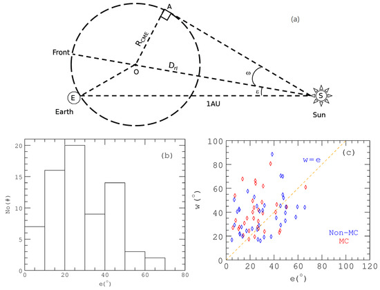
Figure 4.
(a): Sketch Map of CME’s Self-Similar Expansion Model. E means the Earth, S stands for the Sun, Front (F) shows the front of CME, D equals which means the actual propagation distance of CME, is the half-angular width, is the deviation angle and R is the half of face-on width (or radius) of CME [28]. (b): Histogram of CPA or Deviation angle ; (c): Scatter-Plot of the relationship between Deviation angle and Half-Angular Width .
The histogram indicates that ranges from to , and is clustered in the region between and . Specifically, 93% () of are in this range. As expected, the result also suggests that most of the Earth-impacting CMEs are centralized at the solar disk and propagate towards the Earth.
In addition to CPA, the other geometrical parameters of CMEs from GCS also have important effects on whether they could arrive at Earth or not.
Note that the parameters we talk about here consist of face-on angular width (double in Table 1), edge-on width and . For simplification, this work does not explore the influence of edge-on width and , but only discusses the effect of . We assume that a CME moves as a self-similar expansion ball [28], as illustrated in Figure 4a, which is a reasonable and useful assumption in CME propagation studies [55].
The geometric relationships in this sketch map show that the CME can arrive at the Earth without deviating when its half-angular width is not less than the deviation angle, that is, . Figure 4c shows the scatter-plot of and with diamond symbols. The orange dashed line indicates . Based on the previous analysis, CMEs distributed in the region above the dashed line should be able to arrive at the Earth while those in the lower region () should not. Here, about 69% of the CMEs have no less than . Considering that all these CMEs are Earth-impacting, this proportion derived from the above criterion looks fine, but is not so perfect. There are two possible reasons why the other 31% also arrive at Earth. The first reason we consider is that these CMEs have undergone a large deflection in the process of interplanetary space propagation [55,56]. When a CME or flux rope structure that does not satisfy arrives at Earth after deflection, the parts through which the spacecraft pass is their flanks but not the central flux rope structures. So, the in-situ observation may present a non-MC appearance [55]. On the contrary, if a CME arrives at the Earth without deflection (), the in-situ observation will present an MC structure. To test this idea, we divide the events into two groups. One with red diamond symbols represent the CME with MCs observed in-situ, the other with blue diamond symbols represent those with Non-MCs observed in-situ, as shown in Figure 4c. Among those CMEs which satisfy , 24 are MCs and the other 25 are non-MCs. For those CMEs that do not meet , () are MCs, and () are non-MCs. The presence of MC or non-MC appears almost equivalently in both groups. Another reason is that the effects of the error of and need to be taken into account. As mentioned in Section 3, the mean uncertainty of , and is about , and , respectively. The mean uncertainty of has been calculated to be 3.3. Given that the uncertainties differ from one another, although their mean values are not remarkable, it still suggests that there should be more than 69% of Earth-impacting CMEs that satisfy the condition .
In total, is a rough but significant condition for a CME to reach the Earth. Therefore, this criterion should be considered an important part of the space weather forecasting model. On the other hand, there are still some events that do not satisfy our criterion but can be Earth-impacting. It means that this criterion is not a necessary condition. A possible explanation is that they had some deflections during propagation, which cannot be verified by this work because we haven’t derived any large changes for latitude and longitude during the investigated period. It is a subject worthy of further study.
4.3. Simple Kinematics Analysis
Once we know there might be an Earth-impacting CME, it is a matter of cardinal significance to learn when the CME would arrive. So the kinematics of Earth-impacting CMEs is also another important subject for space weather forecasting studies, for which we need to focus on the velocity and acceleration of CMEs at the beginning.
To get a general view of the distribution of the velocity and acceleration of these Earth-impacting CMEs, we plot the histograms for velocity and acceleration as in Figure 5a,b. The average of is km·s and the median is km·s. The distribution of the velocity of CMEs demonstrates that there are not too many high-speed Earth-impacting CMEs during the period we study. For the accelerations, as shown in Figure 5b, they are centralized at 0 m·s, more concretely, about 65% () of CMEs have accelerations of ∼20 m·s. In addition, the average and median values of acceleration are m·s and m·s, respectively. CMEs are decelerating on average, as seen by these two values. It is worth noting that, as shown in Table 1, the uncertainty of is roughly the same as its values, so it can be ignored in most cases. These general views of provide a significant piece of information that most of these CMEs maintain uniform speed or have little change on velocity from 3 to 20 R (LASCO C2: 2.2-6 solar radii; STEREO-COR2: 3-20 solar radii).
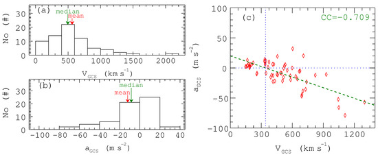
Figure 5.
(a) Histogram of Velocity of GCS Model Fitting Resulting (unit: km·s); (b) Histogram of Acceleration of GCS Model Fitting Resulting (unit: m·s); (c) Scatter-Plot of Velocity and Acceleration.
To reveal the nature of the characteristics of the acceleration, we analyze the correlation between the velocity and the acceleration. As Figure 5c shows, there is an obvious negative correlation between and , with a correlation coefficient (CC) of −0.709. The green dash line in Figure 5c is the linear fitting result. When equals 0 m·s, the corresponding value of is km·s, which represents the average solar wind speed from 3 to 20 R during the investigation period [19]. Our statistical results are consistent with the previous understanding [3,19,24,27,57] that fast CMEs will be hindered and decelerated; conversely, slow CMEs will be dragged and accelerated under the effects of background solar wind.
After analyzing the general characteristics of the velocity and acceleration of Earth-impacting CMEs, we then study the actual propagation time (the actual propagation time mentioned here equals Time_arrive from column 9 in Table 1 minus Time_fit from column 2 in Table 1) of CMEs for a further understanding of their kinematic characteristics and also for establishing the propagation model of CMEs to realize Earth-impacting CMEs forecasting in the future.
As shown in Figure 6, CMEs’ propagation time range from about 1.5 days to about 6 days, which are inversely related to the velocity of CMEs. The green dash dot line shown in Figure 6 is the hyperbolic fitted curve, and the fitting curve equation is
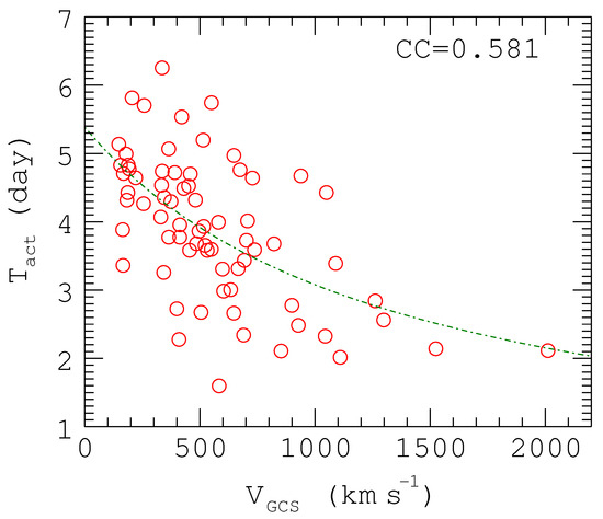
Figure 6.
Scatter-Plot and Hyperbolic Function Fitting Curve of Actual Propagation Time and Velocity : red circles are scatter points and green dash dot line is the result of hyperbolic fitting between and , CC at upper right corner means the correlation coefficient.
The correlation coefficient (CC) of the hyperbolic fitting is 0.581. The coefficient of in Equation (2) is 1.4 , which is comparable to the value in Equation (1) in Wang et al. (2002) [26] which is about 1.14 after unit conversion. The determined value of propagation time using this equation has a maximum deviation of about 51.6 h, a minimum deviation of about 0.1 h, and an average deviation of about 15.2 h. This average value is comparable with previous results [31,58,59,60]. Therefore, it is reasonable to establish a simple propagation model of Earth-impacting CME based on Equation (2).
Although the empirical model mentioned above can obtain a value comparable with previous results, it just represents the general relationship between propagation time and the CMEs’ initial velocities. The details of the CME’s motion are still needed to improve the accuracy of the Earth-impacting CME predictions, which are outside the scope of this empirical statistical model. Besides, it is important to remember that the actual propagation distance for a CME to reach the Earth is not always 1 AU. Sometimes this value could be a bit larger than 1 AU.
As Figure 4a has shown, it is obvious that , which means that CMEs’ fronts have gone beyond 1 AU when they hit the Earth [28]. Using the geometric relationship shown in Figure 4a, we get Equation (3):
Then we can solve the (hereinafter, we use , which means the actual propagation distance to represent ). Note that we remove 22 invalid events () because the simultaneous equation of Equation (3) does not have real roots unless .
After taking the actual propagation distance into account, we can start to analyze the motion of CMEs. Here we use a kinematic model to describe the motion of a CME in the drag-dominated regime [50]. A simplified equation can be represented as
Here, we substitute km·s, , and into Equation (4), based on our previous statistical results of the average background solar wind speed and the values used in Maloney et al. (2010) [50], Shen et al. (2014) [28], Shi et al. (2015) [31] and Dumbovic et al. (2021) [61]. Note that, since we use a quadratic dependence here (), we name Equation (4) the Aerodynamic Drag Model (ADM) [31,50,61,62,63].
Using the aerodynamic drag model, we can calculate the propagation time of these Earth-impacting CMEs by numerical calculation (see Appendix A.2 for detail). The calculation uses the values of initial velocity () computed by the GCS model as the initial value of in Equation (4) and actual propagation distance () computed using Equation (3) as the final value of r. In the process of calculation, we can also obtain the change in velocity and the change in distance. Figure 7 is an example of the velocity change profile and distance change profile for a CME that occurred on 23 May 2010. The black curve in panel (a) shows how the CME’s velocity () changes versus the heliocentric distance of the CME’s front (r) and the black vertical dashed line represents that the actual propagation distance for this CME is about 1.09 (au). In panel (b), the black line shows how the heliocentric distance of CME’s front changes as the propagation time (T) increases, the red vertical dashed line represents that the calculated total propagation time for this CME is about 119.76 h and the blue vertical dashed line shows that the actual propagation time is about 121.62 h. The deviation between these two values is 1.86 h.
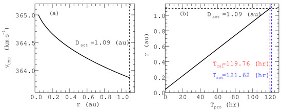
Figure 7.
Numerical calculation results of a CME that occurred on 23 May 2010. (a) velocity profile; (b) heliocentric distance profile.
Then, we compare the actual propagation time (T) and the calculated results (T) of both ADM and the Empirical Statistic Model (ESM, described as Equation (2)) to test their accuracy. Figure 8 shows the comparison results.
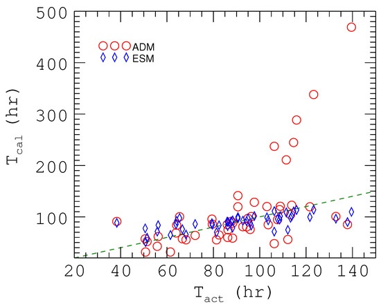
Figure 8.
Scatter-Plot of Calculated Propagation Time and Actual Propagation Time . Red circles are the calculation by aerodynamic drag model; blue diamonds are the calculation by empirical statistic model; green dash line shows the relation .
In Figure 8, red circles represent the calculation by ADM, blue diamonds are the calculation by ESM, the green dashed line shows the relation . A rough comparison of the two models shows that propagation time calculated by ESM seems to have better accordance with the actual value, that is, those diamonds are closer to the dashed line than those circles. Moreover, we use the least square method to calculate the variance between the and , that is, we use the following formula:
In Equation (5), N is the number of these events.
The result is quite similar to the rough glimpse. is about 333.3 while is about 3387.5; the latter is much bigger than the former due to the six events with large , and we can obtain a smaller value if we remove the six events temporarily. The value of is much more affected by outliers; a smaller stands for less fluctuation or less deviation of one model. Considering this aspect, we hold the opinion that ESM is more accurate or more stable than ADM. The expected outperformance [31,61] of ADM over ESM does not occur.
For further analysis, we check the velocity of the six events with large of ADM, which included ·, ·, ·, ·, · and ·. These are the six minimum velocities among all the events involved in the calculation, which have velocities no larger than ·. The calculation by ADM suggests that these small velocity CMEs should be quite slow to arrive at the Earth while the actual propagation times are much shorter, indicating that low speed CMEs may not be suitable for using Equation (4) to describe their motion, or their ADM equations probably need different C, , and even . This phenomenon shows that most suitable constants for Equation (4) may be affected by the velocity; previous studies have tried to analyze the optimal coefficients under different velocities [61]. Other parameters of a CME are also likely to influence the amount of drag from the solar wind [3]. Another possible reason is that there may be other mechanisms by which they accelerate such as two CMEs’ interactions [57,64]. These are follow-up works and will not be discussed here.
5. Conclusions & Discussion
This work is a systematic study and analysis of 71 Earth-impacting CMEs from 21 July 2008 to 11 December 2012. The three-dimensional parameters of these CMEs are obtained using the GCS model. They have been used to analyze the geometric and kinematics characteristics of Earth-impacting CMEs, and an attempt has been made to find a simple propagation model of them. We conclude the following:
- A large majority of the Earth-impacting CMEs are located near the solar disk’s center, which is defined by the coordinates [30S,30N] × [40E,40W]. This conclusion is consistent with previous studies. For example, Hess et al. (2017) [24] found that all the Earth-affecting CMEs are within 45 in latitude from the equator and 36 in longitude from the central meridian. A few Earth-impacting CMEs come from the region far from the solar disk’s center, which shows a possibility for limb events to be Earth-impacting.
- Assuming a radial propagation, the central propagation angle (CPA, or ) of CMEs could represent their deviations. Based on this, we suggest that CMEs with a CPA less than may well be Earth-impacting, which verifies the previous results, such as 86% of FHCMES have a CPA smaller than 50 [29]. If taking CMEs’ other geometric parameters into account, such as the half-angular width (), and considering the effect of the errors, the proportion of Earth-impacting CMEs that satisfy is no less than 69%, which suggests that this inequality should be an important part of Earth-impacting CME forecasting.
- The velocity and acceleration of Earth-impacting CMEs follow each other with a negative correlation owing to the drag from the environment of which the background solar wind is a major part, so we use the v-axis intercept 341 km·s as the average solar wind. This conclusion is reasonable and consistent with other studies [3,19,24,27]. The propagation time is inversely related to velocity, based upon which an empirical formula of CMEs’ propagation can be obtained by hyperbolic fitting. This formula is , which can give, with a good approximation, the propagation time of a CME to determine when it will reach Earth. However, the empirical statistical model only represents the general relationship between propagation time and CMEs’ initial velocities; it can not describe the detail of the motion of CMEs, so we introduce an aerodynamic drag model to conduct more analysis. A rough comparison of these two models shows that the deviations between the calculated results and actual values of our empirical statistical model are smaller than those of the aerodynamic drag model, and the equation of the latter we use has low performance in low speed events. The matter needs further investigation.
In general, this work builds up a database based on GCS model fitting results for the geometric parameters of Earth-impacting CMEs, which is useful for further studies. This work also conducts preliminary statistical work to analyze the parameter we obtain and also achieves an empirical model for Earth-impacting CME forecasting.
For discussion, a manual, systematic study of many CMEs free from bias is a challenge due to the lack of a uniform and precise definition of a CME, and the subjective nature of the measurement process when performed by a human operator [65]. The main errors in this work are the artificial fitting process in the GCS model fitting; this problem should be overcome by a repeated fitting process and averaging of the results. Another unavoidable error is missing data in the coronagraphs, which makes the fitting less accurate. In addition, owing to the assumption that the CME is an ideal flux rope in the GCS model, the geometric description of CMEs becomes better. However, this assumption also limits a richer description of CMEs, leading to the inapplicability of the GCS model for more complex shaped CMEs. Therefore, it is also unavoidable that some error may exist in the fitting results, especially for those parameters that involve CMEs’ shapes. For example, above 30 (solar radii), the front of flux rope CMEs becomes distorted because of interactions with the ambient solar wind [3,66]—the GCS model is not capable of reproducing such behavior [40]. In total, the GCS model itself also contributes to errors. Recently, some new methods have been developed that aim to eliminate model defects or manual errors, which can be used to estimate a CME’s propagation (e.g., CORSET3D [65], iCAF [67] and ELEvoHI [68]).
Moreover, the study of Patsourakos et al. (2010) [69] shows that, by not restraining the foot point to be at the center of the Sun, it allows better GCS model fitting for the CMEs with propagation directions not perpendicular to the solar surface (e.g., the case on 21 June 2011 from Heinemann et al. 2019 [70], the case on 23 July 2017 from Dumbovic et al. 2019 [71]). This finding can be helpful to our further study of a more specific and more vision-broad analysis of CMEs’ propagation, considering that our present work only used the data of SOHO/LASCO/C2 and STEREO/SECCHI/COR2. A more complete propagation process of a CME from its eruption to the interplanetary space can be analyzed by combining the data of EUVI, COR1, COR2, HI1, and HI2, in which case the more complex process of a CME’s motion needs to be considered [72].
In addition to various geometric models or methods, a numerical simulation based on magnetohydrodynamics is also a particularly popular method for studying CMEs in recent years. For example, Shen et al. investigated the acceleration and deceleration of CMEs on 28–31 March 2001 with a 3D COIN-TVD MHD model [57], and they also investigated the influence of the CME’s initial parameters on the simulation results [73,74]. These MHD numerical simulations can study CMEs in more detail, especially CMEs with complex structures that are difficult to analyze with most geometric methods, which is conducive to our understanding of the initial parameters and propagation process of CMEs.
Recently, some new solar probe spacecraft have been launched (e.g., Parker Solar Probe [75] and Solar Orbiter [76]), and other concepts for monitoring the Sun and the inner heliosphere have been proposed by Wang et al. (2020) [77] (Solar Ring mission). With the help of the observation of PSP, Solar Orbiter, and possible Solar Ring, we can observe the generation, propagation and interaction of CMEs from more perspectives (e.g., Braga and Vourlidas 2021 [78]), and some more accurate forecast models of Earth-impacting CMEs can be established.
Author Contributions
Conceptualization, Z.Z. and C.S.; methodology, Z.Z., C.S., D.M. and Y.C.; software, Z.Z., D.M. and J.L.; validation, Z.Z., C.S. and Y.C.; formal analysis, Z.Z. and C.S.; investigation, Z.Z., Y.C.; data curation, Z.Z.; writing—original draft preparation, Z.Z.; writing—review and editing, Z.Z., C.S., D.M., Y.C., M.X., J.L. and Y.W.; funding acquisition, C.S., Y.C. and M.X. All authors have read and agreed to the published version of the manuscript.
Funding
This work is supported by grants from NSFC(41822405, 41474164, 41904151), the Strategic Priority Program of CAS (XDB41000000), Anhui Provincial Natural Science Foundation (1908085MD107), Project funded by China Postdoctoral Science Foundation (2019M652194).
Institutional Review Board Statement
Not applicable.
Informed Consent Statement
Not applicable.
Data Availability Statement
The processed data and program underlying this article will be shared on request to the corresponding author.
Acknowledgments
We acknowledge the use of the CME catalog, the data from SECCHI instruments on STEREO and LASCO on SOHO. The CME catalog is generated and maintained at the CDAW Data Center by NASA and the Catholic University of America in cooperation with the Naval Research Laboratory. STEREO is the third mission in NASA Solar Terrestrial Probes program, and SOHO is a mission of international cooperation between ESA and NASA.
Conflicts of Interest
The authors declare no conflict of interest.
Appendix A
Appendix A.1. ICME-CME List
The ICME-CME list we got is shown in Table A1. Columns from left to right are the sequence number of the event (No.), initial time observed by STEREO-COR2, initial time observed by SOHO-LASCO-C2, position angle measured from Solar North in degrees (counter-clockwise; PA), the sky-plane width of CMEs (Width) in degrees, linear speed of CMEs (V) in km·, acceleration of CMEs (Acc) in m·, start of the ejecta observed by WIND, and mean velocity in the ejecta (V) in km·. The parameters ’Initial time by C2’, PA, Width, V, and Acc are all from the CDAW SOHO/LASCO CME catalog (https://cdaw.gsfc.nasa.gov/CME_list/index.html (accessed on 23 July 2021)) [20]. Symbols ‘’ represent that there are no corresponding data.
It is worthwhile to note that ‘Initial time by COR2’ or ‘Initial time by C2’ are not always the same as ‘Time_fit’ in Table 1 because we start GCS fitting when all three spacecraft can observe the CME clearly. And, the width, V, and Acc in Table A1 are different from the corresponding parameter we got from GCS fitting since the former are the results from only C2 observation but the latter is the three-dimensional parameters.
Table A1.
ICME-CME list.
Table A1.
ICME-CME list.
| No. | Initial Time by COR2 | Initial Time by C2 | PA | Width | V | Acc | Start of the Ejecta | V |
|---|---|---|---|---|---|---|---|---|
| 1 | 2008/07/21T11:38:30 | 2008/07/21 13:31 | 228 | 47 | 200 | 11 | 2008-07-25T13:17:20 | 408 |
| 2 | 2008/12/12T07:37:00 | 2008/12/12 09:30 | 154 | 8 | 281 | 29.4 | 2008-12-17T03:24:45 | 339 |
| 3 | 2009/01/21T22:07:00 | 2009/01/21 18:54 | 253 | 73 | 220 | 4.5 | 2009-01-26T04:59:15 | 348 |
| 4 | 2009/06/23T00:37:00 | 2009/06/22 22:30 | 241 | 47 | 126 | 1.9 | 2009-06-27T18:36:00 | 388 |
| 5 | 2009/11/09T17:24:00 | −−− | −−− | −−− | −−− | −−− | 2009-11-14T10:41:15 | 322 |
| 6 | 2009/12/30T14:54:00 | 2009/12/30 10:30 | 275 | 65 | 173 | 4 | 2010-01-01T22:03:00 | 296 |
| 7 | 2010/02/03T01:24:00 | −−− | −−− | −−− | −−− | −−− | 2010-02-07T23:17:15 | 360 |
| 8 | 2010/02/06T19:54:00 | 2010/02/06 20:06 | 95 | 97 | 240 | − 0.1 | 2010-02-12T13:16:58 | 326 |
| 9 | 2010/02/07T03:24:00 | 2010/02/07 04:06 | Halo | 360 | 421 | 0.5 | 2010-02-11T11:33:00 | 358 |
| 10 | 2010/02/08T09:24:00 | 2010/02/08 06:30 | 85 | 99 | 153 | 0 | 2010-02-13T22:14:14 | 308 |
| 11 | 2010/02/10T17:24:00 | 2010/02/10 17:30 | 90 | 58 | 538 | 4.3 | 2010-02-15T11:53:48 | 308 |
| 12 | 2010/02/12T11:54:00 | 2010/02/12 13:42 | Halo | 360 | 509 | −18.3 | 2010-02-16T04:01:52 | 318 |
| 13 | 2010/02/13T23:08:00 | 2010/02/13 19:54 | 290 | 126 | 247 | 8.6 | 2010-02-19T19:57:00 | 396 |
| 14 | 2010/04/03T10:08:00 | 2010/04/03 10:33 | Halo | 360 | 668 | −1 | 2010-04-05T13:09:45 | 639 |
| 15 | 2010/04/06T01:39:00 | 2010/04/06 02:30 | 125 | 9 | 378 | −34.9 | 2010-04-09T19:07:30 | 448 |
| 16 | 2010/04/08T03:54:00 | 2010/04/08 04:54 | 249 | 160 | 264 | −2.2 | 2010-04-12T01:07:30 | 409 |
| 17 | 2010/04/18T23:24:00 | 2010/04/18 20:30 | 257 | 100 | 381 | 17.1 | 2010-04-22T05:06:00 | 399 |
| 18 | 2010/05/23T17:24:00 | 2010/05/23 18:06 | Halo | 360 | 258 | 3.2 | 2010-05-28T19:43:30 | 354 |
| 19 | 2010/06/16T11:24:00 | 2010/06/16 04:06 | 341 | 47 | 198 | 0.6 | 2010-06-21T07:30:00 | 365 |
| 20 | 2010/06/16T21:24:00 | 2010/06/16 14:54 | 61 | 153 | 236 | 6.5 | 2010-06-21T07:30:00 | 365 |
| 21 | 2010/08/01T08:24:00 | 2010/08/01 13:42 | Halo | 360 | 850 | 247 | 2010-08-04T09:54:00 | 537 |
| 22 | 2011/01/19T11:54:00 | −−− | −−− | −−− | −−− | −−− | 2011-01-24T10:18:11 | 367 |
| 23 | 2011/01/21T13:24:00 | 2011/01/21 13:25 | 341 | 144 | 117 | 3.1 | 2011-01-25T00:20:48 | 349 |
| 24 | 2011/01/30T11:54:00 | 2011/01/30 12:36 | 184 | 264 | 120 | 3.3 | 2011-02-04T09:29:15 | 405 |
| 25 | 2011/03/25T06:54:00 | 2011/03/25 08:48 | 107 | 59 | 320 | 1.2 | 2011-03-30T00:21:05 | 358 |
| 26 | 2011/05/25T05:39:00 | 2011/05/25 05:24 | 320 | 38 | 276 | 2.8 | 2011-05-28T05:33:00 | 517 |
| 27 | 2011/05/25T13:39:00 | 2011/05/25 13:25 | 321 | 78 | 561 | −2.6 | 2011-05-28T05:33:00 | 517 |
| 28 | 2011/06/01T18:24:00 | 2011/06/01 18:36 | 112 | 189 | 361 | 4.1 | 2011-06-05T01:57:00 | 513 |
| 29 | 2011/07/11T11:24:00 | 2011/07/11 12:00 | 213 | 53 | 266 | 8.6 | 2011-07-15T06:29:15 | 415 |
| 30 | 2011/08/02T06:54:00 | 2011/08/02 06:36 | 288 | 268 | 712 | −15.5 | 2011-08-06T22:16:30 | 539 |
| 31 | 2011/09/13T23:24:00 | 2011/09/14 00:00 | 334 | 242 | 408 | 3.2 | 2011-09-17T15:37:30 | 441 |
| 32 | 2011/09/14T21:24:00 | 2011/09/14 20:12 | 239 | 131 | 375 | 9 | 2011-09-18T12:24:00 | 442 |
| 33 | 2011/10/01T10:24:00 | 2011/10/01 09:36 | 317 | 203 | 448 | −3.3 | 2011-10-05T09:49:30 | 453 |
| 34 | 2011/10/02T01:24:00 | 2011/10/02 02:00 | 167 | 103 | 259 | 0.6 | 2011-10-06T14:06:00 | 371 |
| 35 | 2011/10/22T01:24:00 | 2011/10/22 01:25 | Halo | 360 | 593 | 9.5 | 2011-10-25T00:32:37 | 472 |
| 36 | 2011/10/26T12:24:00 | 2011/10/26 10:00 | 298 | 158 | 270 | 5.1 | 2011-10-31T00:58:30 | 389 |
| 37 | 2011/11/26T07:24:00 | 2011/11/26 07:12 | Halo | 360 | 933 | 9 | 2011-11-29T01:50:15 | 449 |
| 38 | 2011/12/26T11:54:00 | 2011/12/26 11:48 | 340 | 277 | 736 | −19.3 | 2011-12-29T22:21:00 | 384 |
| 39 | 2012/01/19T15:24:00 | 2012/01/19 14:36 | Halo | 360 | 1120 | 54.1 | 2012-01-22T23:57:45 | 418 |
| 40 | 2012/02/09T21:54:00 | 2012/02/09 21:17 | Halo | 360 | 659 | 1.2 | 2012-02-14T20:36:22 | 384 |
| 41 | 2012/02/10T20:24:00 | 2012/02/10 20:00 | Halo | 360 | 533 | 3.8 | 2012-02-16T14:14:37 | 335 |
| 42 | 2012/02/24T03:24:00 | 2012/02/24 03:46 | 341 | 341 | 800 | 13.3 | 2012-02-27T18:04:30 | 439 |
| 43 | 2012/03/03T19:24:00 | 2012/03/03 18:36 | 49 | 192 | 1078 | −17.3 | 2012-03-06T06:30:00 | 380 |
| 44 | 2012/03/07T00:39:00 | 2012/03/07 00:24 | Halo | 360 | 2684 | −88.2 | 2012-03-09T03:08:31 | 563 |
| 45 | 2012/03/13T17:39:00 | 2012/03/13 17:36 | Halo | 360 | 1884 | 45.6 | 2012-03-15T21:00:00 | 685 |
| 46 | 2012/03/20T16:24:00 | 2012/03/30 14:46 | 44 | 141 | 584 | −1.9 | 2012-04-04T20:06:00 | 335 |
| 47 | 2012/04/19T15:39:00 | 2012/04/19 15:12 | 138 | 142 | 540 | 7.9 | 2012-04-23T16:43:18 | 373 |
| 48 | 2012/04/23T18:24:00 | 2012/04/23 18:24 | Halo | 360 | 528 | −1.1 | 2012-04-26T02:35:37 | 541 |
| 49 | 2012/04/29T10:39:00 | 2012/04/29 09:36 | 61 | 145 | 475 | 2.2 | 2012-05-04T03:27:00 | 310 |
| 50 | 2012/05/11T23:53:00 | 2012/05/12 00:00 | Halo | 360 | 805 | −6.6 | 2012-05-16T16:07:30 | 369 |
| 41 | 2012/05/28T05:24:00 | 2012/05/28 08:00 | 323 | 79 | 621 | 76.1 | 2012-06-01T19:30:00 | 359 |
| 52 | 2012/05/28T11:24:00 | 2012/05/28 11:36 | 292 | 74 | 115 | −2.7 | 2012-06-02T14:54:00 | 334 |
| 53 | 2012/06/06T20:24:00 | 2012/06/06 20:36 | 180 | 173 | 494 | −2.3 | 2012-06-08T11:00:16 | 488 |
| 54 | 2012/06/14T13:54:00 | 2012/06/14 14:12 | Halo | 360 | 987 | −1.2 | 2012-06-16T22:12:00 | 446 |
| 55 | 2012/07/01T06:54:00 | 2012/07/01 06:12 | 154 | 181 | 423 | −1.5 | 2012-07-05T01:14:15 | 491 |
| 56 | 2012/07/06T23:24:00 | 2012/07/06 23:24 | Halo | 360 | 1828 | −56.1 | 2012-07-08T23:46:30 | 413 |
| 57 | 2012/07/12T16:39:00 | 2012/07/12 16:48 | Halo | 360 | 885 | 195.6 | 2012-07-15T06:22:30 | 516 |
| 58 | 2012/08/14T03:24:00 | 2012/08/14 04:36 | 276 | 150 | 198 | 2 | 2012-08-16T21:49:30 | 413 |
| 59 | 2012/08/26T08:24:00 | 2012/08/26 07:24 | 25 | 86 | 208 | 1.5 | 2012-08-30T18:40:30 | 400 |
| 60 | 2012/08/31T19:24:00 | 2012/08/31 19:24 | 334 | 157 | 278 | 7.3 | 2012-09-04T16:38:26 | 446 |
| 61 | 2012/08/31T20:24:00 | 2012/08/31 20:00 | Halo | 360 | 1442 | 2 | 2012-09-05T06:39:22 | 505 |
| 62 | 2012/09/02T03:24:00 | 2012/09/02 04:00 | Halo | 360 | 538 | −6.9 | 2012-09-06T02:15:00 | 425 |
| 63 | 2012/09/02T09:54:00 | 2012/09/02 09:36 | 287 | 173 | 404 | 4.3 | 2012-09-06T18:27:00 | 391 |
| 64 | 2012/09/24T09:24:00 | 2012/09/24 04:36 | 90 | 81 | 245 | 3.7 | 2012-09-30T12:29:15 | 328 |
| 65 | 2012/09/28T00:24:00 | 2012/09/28 00:12 | Halo | 360 | 947 | −27.1 | 2012-10-01T17:10:30 | 358 |
| 66 | 2012/10/05T02:39:00 | 2012/10/05 02:48 | 258 | 284 | 612 | 21.2 | 2012-10-08T17:22:30 | 391 |
| 67 | 2012/10/27T16:24:00 | 2012/10/27 16:48 | Halo | 360 | 317 | 9.1 | 2012-10-31T23:30:45 | 344 |
| 68 | 2012/11/09T15:24:00 | 2012/11/09 15:12 | 175 | 276 | 559 | 4 | 2012-11-13T07:43:30 | 380 |
| 69 | 2012/11/20T12:24:00 | 2012/11/20 12:00 | Halo | 360 | 619 | 2.6 | 2012-11-24T12:45:00 | 379 |
| 70 | 2012/11/23T14:24:00 | 2012/12/11 15:36 | Halo | 360 | 519 | −1.9 | 2012-11-26T21:47:15 | 415 |
| 71 | 2012/12/11T15:24:00 | 2012/11/24 13:48 | 63 | 60 | 380 | −40.2 | 2012-12-14T07:34:30 | 324 |
Notes: See Appendix A.1 for a detailed description of this table.
Appendix A.2. Aerodynamic Drag Model Calculation
The following pseudo-code gives the implementation of aerodynamic drag model calculation based on Equation (4). The input is the average initial velocity we got, which presents the velocity of the midpoint in the fitting height range. So, another input is the heliocentric distance in the fitting height range. , and mean the CME velocity, heliocentric distance and total propagation time in the ith step, respectively. and means the increment of CME velocity and heliocentric distance in the ith step, respectively. is a fixed value which means the increment of total propagation time for each step. is the actual propagation distance for each event. is the final calculation results of CME total propagation time.
The pseudo-code is given here:
| Algorithm A1 Aerodynamic Drag Model Calculation |
 |
References
- Gosling, J.; Hildner, E.; MacQueen, R.; Munro, R.; Poland, A.; Ross, C. Mass ejections from the Sun: A view from Skylab. J. Geophys. Res. 1974, 79, 4581–4587. [Google Scholar] [CrossRef]
- Hundhausen, A. An introduction. Coronal Mass Ejections 1997, 99, 1–7. [Google Scholar]
- Temmer, M. Space weather: The solar perspective An update to Schwenn (2006). Living Rev. Sol. Phys. 2021, 18. [Google Scholar] [CrossRef]
- Ogilvie, K.W.; Chornay, D.J.; Fritzenreiter, R.J.; Hunsaker, F.; Keller, J.; Lobell, J.; Miller, G.; Scudder, J.D.; Sittler, E.C.; Torbert, R.B.; et al. Swe, a comprehensive plasma instrument for the wind spacecraft. Space Sci. Rev. 1995, 71, 55–77. [Google Scholar] [CrossRef]
- Klein, L.W.; Burlaga, L.F. Interplanetary magnetic clouds At 1 AU. J. Geophys. Res. Space Phys. 1982, 87, 613–624. [Google Scholar] [CrossRef]
- Richardson, I.G.; Cane, H.V. Regions of abnormally low proton temperature in the solar wind (1965–1991) and their association with ejecta. J. Geophys. Res. Space Phys. 1995, 100, 23397–23412. [Google Scholar] [CrossRef]
- Burlaga, L.F.; Skoug, R.M.; Smith, C.W.; Webb, D.F.; Zurbuchen, T.H.; Reinard, A. Fast ejecta during the ascending phase of solar cycle 23: ACE observations, 1998–1999. J. Geophys. Res. Space Phys. 2001, 106, 20957–20977. [Google Scholar] [CrossRef]
- Bame, S.J.; Asbridge, J.R.; Feldman, W.C.; Gosling, J.T.; Zwickl, R.D. Bi-directional streaming of solar wind electrons >80 eV: ISEE evidence for a closed-field structure within the driver gas of an interplanetary shock. Geophys. Res. Lett. 1981, 8, 173–176. [Google Scholar] [CrossRef]
- Bame, S.; Asbridge, J.; Feldman, W.; Fenimore, E.; Gosling, J. Solar-wind heavy-ions from flare-heated coronal plasma. Sol. Phys. 1979, 62, 179–201. [Google Scholar] [CrossRef]
- Henke, T.; Woch, J.; Schwenn, R.; Mall, U.; Gloeckler, G.; von Steiger, R.; Forsyth, R.; Balogh, A. Ionization state and magnetic topology of coronal mass ejections. J. Geophys. Res.-Space Phys. 2001, 106, 10597–10613. [Google Scholar] [CrossRef]
- Ipavich, F.M.; Galvin, A.B.; Gloeckler, G.; Hovestadt, D.; Bame, S.J.; Klecker, B.; Scholer, M.; Fisk, L.A.; Fan, C.Y. Solar wind Fe and CNO measurements in high-speed flows. J. Geophys. Res. Space Phys. 1986, 91, 4133–4141. [Google Scholar] [CrossRef]
- Schwenn, R.; Rosenbauer, H.; Mühlhäuser, K.H. Singly-ionized helium in the driver gas of an interplanetary shock wave. Geophys. Res. Lett. 1980, 7, 201–204. [Google Scholar] [CrossRef]
- Burlaga, L.; Sittler, E.; Mariani, F.; Schwenn, R. Magnetic loop behind an interplanetary shock: Voyager, Helios, and IMP 8 observations. J. Geophys. Res. Space Phys. 1981, 86, 6673–6684. [Google Scholar] [CrossRef]
- Richardson, I.G.; Cane, H.V. Near-Earth Interplanetary Coronal Mass Ejections During Solar Cycle 23 (1996-aEuro parts per thousand 2009): Catalog and Summary of Properties. Sol. Phys. 2010, 264, 189–237. [Google Scholar] [CrossRef]
- Jian, L.K.; Russell, C.T.; Luhmann, J.G.; Galvin, A.B. STEREOObservations of Interplanetary Coronal Mass Ejections in 2007–2016. Astrophys. J. 2018, 855, 114. [Google Scholar] [CrossRef]
- Chi, Y.; Shen, C.; Wang, Y.; Xu, M.; Ye, P.; Wang, S. Statistical study of the interplanetary coronal mass ejections from 1995 to 2015. Sol. Phys. 2016, 291, 2419–2439. [Google Scholar] [CrossRef]
- Gonzalez, W.; Joselyn, J.A.; Kamide, Y.; Kroehl, H.W.; Rostoker, G.; Tsurutani, B.; Vasyliunas, V. What is a geomagnetic storm? J. Geophys. Res. Space Phys. 1994, 99, 5771–5792. [Google Scholar] [CrossRef]
- Shen, C.L.; Chi, Y.T.; Wang, Y.M.; Xu, M.J.; Wang, S. Statistical comparison of the ICME’s geoeffectiveness of different types and different solar phases from 1995 to 2014. J. Geophys. Res.-Space Phys. 2017, 122, 5931–5948. [Google Scholar] [CrossRef]
- Gopalswamy, N. Coronal mass ejections of solar cycle 23. J. Astrophys. Astron. 2006, 27, 243–254. [Google Scholar] [CrossRef]
- Gopalswamy, N.; Yashiro, S.; Michalek, G.; Stenborg, G.; Vourlidas, A.; Freeland, S.; Howard, R. The soho/lasco cme catalog. Earth Moon Planets 2009, 104, 295–313. [Google Scholar] [CrossRef]
- Ameri, D.; Valtonen, E. Investigation of the Geoeffectiveness of Disk-Centre Full-Halo Coronal Mass Ejections. Sol. Phys. 2017, 292, 79. [Google Scholar] [CrossRef]
- Besliu-Ionescu, D.; Mierla, M. Geoeffectiveness Prediction of CMEs. Front. Astron. Space Sci. 2021, 8, 79. [Google Scholar] [CrossRef]
- Goswami, A. Studying the properties of interplanetary counterpart of halo-CMEs and their influences on Dst index. Adv. Space Res. 2019, 64, 287–298. [Google Scholar] [CrossRef]
- Hess, P.; Zhang, J. A Study of the Earth-Affecting CMEs of Solar Cycle 24. Sol. Phys. 2017, 292, 80. [Google Scholar] [CrossRef]
- Soni, S.L.; Yadav, M.L.; Gupta, R.S.; Verma, P.L. Exhaustive study of three-time periods of solar activity due to single active regions: Sunspot, flare, CME, and geo-effectiveness characteristics. Astrophys. Space Sci. 2020, 365, 189. [Google Scholar] [CrossRef]
- Wang, Y.; Ye, P.; Wang, S.; Zhou, G.; Wang, J. A statistical study on the geoeffectiveness of Earth-directed coronal mass ejections from March 1997 to December 2000. J. Geophys. Res. Space Phys. 2002, 107, SSH-2. [Google Scholar] [CrossRef]
- Wang, Y.M.; Shen, C.L.; Wang, S.; Ye, P.Z. Deflection of coronal mass ejection in the interplanetary medium. Sol. Phys. 2004, 222, 329–343. [Google Scholar] [CrossRef]
- Shen, C.; Wang, Y.; Pan, Z.; Miao, B.; Ye, P.; Wang, S. Full-halo coronal mass ejections: Arrival at the Earth. J. Geophys. Res. Space Phys. 2014, 119, 5107–5116. [Google Scholar] [CrossRef]
- Shen, C.; Wang, Y.; Pan, Z.; Zhang, M.; Ye, P.; Wang, S. Full halo coronal mass ejections: Do we need to correct the projection effect in terms of velocity? J. Geophys. Res. Space Phys. 2013, 118, 6858–6865. [Google Scholar] [CrossRef]
- Bhardwaj, S.; Khan, P.A.; Atulkar, R.; Purohit, P.K. Investigation of geo-effective properties of halo coronal mass ejections. Russ. J. Earth Sci. 2018, 18. [Google Scholar] [CrossRef]
- Shi, T.; Wang, Y.K.; Wan, L.F.; Cheng, X.; Ding, M.D.; Zhang, J. Predicting the arrival time of coronal mass ejections with the graduated cylindrical shell and drag force model. Astrophys. J. 2015, 806, 271. [Google Scholar] [CrossRef]
- Xie, H.; Ofman, L.; Lawrence, G. Cone model for halo CMEs: Application to space weather forecasting. J. Geophys. Res. Space Phys. 2004, 109. [Google Scholar] [CrossRef]
- Xue, X.; Wang, C.; Dou, X. An ice-cream cone model for coronal mass ejections. J. Geophys. Res. Space Phys. 2005, 110. [Google Scholar] [CrossRef]
- Brueckner, G.; Howard, R.; Koomen, M.; Korendyke, C.; Michels, D.; Moses, J.; Socker, D.; Dere, K.; Lamy, P.; Llebaria, A.; et al. The large angle spectroscopic coronagraph (LASCO). In The SOHO Mission; Springer: Berlin/Heidelberg, Germany, 1995; pp. 357–402. [Google Scholar]
- Delaboudiniere, J.; Artzner, G.; Brunaud, J.; Gabriel, A.; Hochedez, J.; Millier, F.; Song, X.; Au, B.; Dere, K.; Howard, R.; et al. EIT: Extreme-ultraviolet imaging telescope for the SOHO mission. Sol. Phys. 1995, 162, 291–312. [Google Scholar] [CrossRef]
- Domingo, V.; Fleck, B.; Poland, A.I. The SOHO mission: An overview. Sol. Phys. 1995, 162, 1–37. [Google Scholar] [CrossRef]
- Kaiser, M.L.; Kucera, T.; Davila, J.; Cyr, O.S.; Guhathakurta, M.; Christian, E. The STEREO mission: An introduction. Space Sci. Rev. 2008, 136, 5–16. [Google Scholar] [CrossRef]
- Thernisien, A.; Howard, R.; Vourlidas, A. Modeling of flux rope coronal mass ejections. Astrophys. J. 2006, 652, 763. [Google Scholar] [CrossRef]
- Thernisien, A.; Vourlidas, A.; Howard, R. Forward modeling of coronal mass ejections using STEREO/SECCHI data. Sol. Phys. 2009, 256, 111–130. [Google Scholar] [CrossRef]
- Thernisien, A. Implementation of the graduated cylindrical shell model for the three-dimensional reconstruction of coronal mass ejections. Astrophys. J. Suppl. Ser. 2011, 194, 33. [Google Scholar] [CrossRef]
- Temmer, M.; Preiss, S.; Veronig, A. CME projection effects studied with STEREO/COR and SOHO/LASCO. Sol. Phys. 2009, 256, 183–199. [Google Scholar] [CrossRef]
- Lugaz, N.; Vourlidas, A.; Roussev, I. Deriving the radial distances of wide coronal mass ejections from elongation measurements in the heliosphere-application to CME-CME interaction. arXiv 2009, arXiv:0909.0534. [Google Scholar] [CrossRef]
- Lugaz, N.; Hernandez-Charpak, J.; Roussev, I.; Davis, C.; Vourlidas, A.; Davies, J. Determining the azimuthal properties of coronal mass ejections from multi-spacecraft remote-sensing observations with STEREO SECCHI. Astrophys. J. 2010, 715, 493. [Google Scholar] [CrossRef]
- Liu, Y.D.; Luhmann, J.G.; Möstl, C.; Martinez-Oliveros, J.C.; Bale, S.D.; Lin, R.P.; Harrison, R.A.; Temmer, M.; Webb, D.F.; Odstrcil, D. Interactions between coronal mass ejections viewed in coordinated imaging and in situ observations. Astrophys. J. Lett. 2012, 746, L15. [Google Scholar] [CrossRef]
- Feng, L.; Inhester, B.; Wei, Y.; Gan, W.; Zhang, T.; Wang, M. Morphological evolution of a three-dimensional coronal mass ejection cloud reconstructed from three viewpoints. Astrophys. J. 2012, 751, 18. [Google Scholar] [CrossRef]
- de Koning, C.A.; Pizzo, V.; Biesecker, D. Geometric localization of CMEs in 3D space using STEREO beacon data: First results. Sol. Phys. 2009, 256, 167–181. [Google Scholar] [CrossRef]
- Mierla, M.; Inhester, B.; Marqué, C.; Rodriguez, L.; Gissot, S.; Zhukov, A.; Berghmans, D.; Davila, J. On 3D reconstruction of coronal mass ejections: I. Method description and application to SECCHI-COR data. Sol. Phys. 2009, 259, 123. [Google Scholar] [CrossRef]
- Lugaz, N. Accuracy and limitations of fitting and stereoscopic methods to determine the direction of coronal mass ejections from heliospheric imagers observations. Sol. Phys. 2010, 267, 411–429. [Google Scholar] [CrossRef]
- Feng, L.; Inhester, B.; Mierla, M. Comparisons of CME morphological characteristics derived from five 3D reconstruction methods. Sol. Phys. 2013, 282, 221–238. [Google Scholar] [CrossRef][Green Version]
- Maloney, S.A.; Gallagher, P.T. Solar wind drag and the kinematics of interplanetary coronal mass ejections. Astrophys. J. Lett. 2010, 724, L127. [Google Scholar] [CrossRef]
- Chi, Y.T.; Zhang, J.; Shen, C.L.; Hess, P.; Liu, L.J.; Mishra, W.; Wang, Y.M. Observational Study of an Earth-affecting Problematic ICME from STEREO. Astrophys. J. 2018, 863, 108. [Google Scholar] [CrossRef]
- Sheeley, N.R.; Walters, J.H.; Wang, Y.M.; Howard, R.A. Continuous tracking of coronal outflows: Two kinds of coronal mass ejections. J. Geophys. Res.-Space Phys. 1999, 104, 24739–24767. [Google Scholar] [CrossRef]
- Howard, R.; Moses, J.; Vourlidas, A.; Newmark, J.; Socker, D.; Plunkett, S.; Korendyke, C.; Cook, J.; Hurley, A.; Davila, J.; et al. Sun Earth connection coronal and heliospheric investigation (SECCHI). Space Sci. Rev. 2008, 136, 67. [Google Scholar] [CrossRef]
- Cane, H.V.; Richardson, I.G.; St. Cyr, O.C. Coronal mass ejections, interplanetary ejecta and geomagnetic storms. Geophys. Res. Lett. 2000, 27, 3591–3594. [Google Scholar] [CrossRef]
- Luhmann, J.G.; Gopalswamy, N.; Jian, L.K.; Lugaz, N. ICME Evolution in the Inner Heliosphere Invited Review. Sol. Phys. 2020, 295, 61. [Google Scholar] [CrossRef]
- Lugaz, N.; Temmer, M.; Wang, Y.M.; Farrugia, C.J. The Interaction of Successive Coronal Mass Ejections: A Review. Sol. Phys. 2017, 292, 64. [Google Scholar] [CrossRef]
- Shen, F.; Wu, S.T.; Feng, X.S.; Wu, C.C. Acceleration and deceleration of coronal mass ejections during propagation and interaction. J. Geophys. Res.-Space Phys. 2012, 117. [Google Scholar] [CrossRef]
- Gopalswamy, N.; Lara, A.; Yashiro, S.; Kaiser, M.L.; Howard, R.A. Predicting the 1-AU arrival times of coronal mass ejections. J. Geophys.-Res.-Space Phys. 2001, 106, 29207–29217. [Google Scholar] [CrossRef]
- Owens, M.; Cargill, P. Non-radial solar wind flows induced by the motion of interplanetary coronal mass ejections. Ann. Geophys. 2004, 22, 4397–4406. [Google Scholar] [CrossRef][Green Version]
- Vrsnak, B.; Temmer, M.; Zic, T.; Taktakishvili, A.; Dumbovic, M.; Mostl, C.; Veronig, A.M.; Mays, M.L.; Odstrcil, D. Heliospheric propagation of coronal mass ejections: Comparison of numerical wsa-enlil plus cone model and analytical drag-based model. Astrophys. J. Suppl. Ser. 2014, 213, 21. [Google Scholar] [CrossRef]
- Dumbovic, M.; Calogovic, J.; Martinic, K.; Vrsnak, B.; Sudar, D.; Temmer, M.; Veronig, A. Drag-Based Model (DBM) Tools for Forecast of Coronal Mass Ejection Arrival Time and Speed. Front. Astron. Space Sci. 2021, 8. [Google Scholar] [CrossRef]
- Vrsnak, B.; Zic, T.; Vrbanec, D.; Temmer, M.; Rollett, T.; Mostl, C.; Veronig, A.; Calogovic, J.; Dumbovic, M.; Lulic, S.; et al. Propagation of Interplanetary Coronal Mass Ejections: The Drag-Based Model. Sol. Phys. 2013, 285, 295–315. [Google Scholar] [CrossRef]
- Byrne, J.P.; Maloney, S.A.; McAteer, R.T.J.; Refojo, J.M.; Gallagher, P.T. Propagation of an Earth-directed coronal mass ejection in three dimensions. Nat. Commun. 2010, 1, 74. [Google Scholar] [CrossRef] [PubMed]
- Shen, C.L.; Wang, Y.M.; Wang, S.; Liu, Y.; Liu, R.; Vourlidas, A.; Miao, B.; Ye, P.Z.; Liu, J.J.; Zhou, Z.J. Super-elastic collision of large-scale magnetized plasmoids in the heliosphere. Nat. Phys. 2012, 8, 923–928. [Google Scholar] [CrossRef]
- Braga, C.R.; Dal Lago, A.; Echer, E.; Stenborg, G.; de Mendonca, R.R.S. Pseudo-automatic Determination of Coronal Mass Ejections’ Kinematics in 3D. Astrophys. J. 2017, 842, 134. [Google Scholar] [CrossRef]
- Chi, Y.; Scott, C.; Shen, C.; Barnard, L.; Owens, M.; Xu, M.; Zhang, J.; Jones, S.; Zhong, Z.; Yu, B.; et al. Modeling the Observed Distortion of Multiple (Ghost) CME Fronts in STEREO Heliospheric Imagers. Astrophys. J. Lett. 2021, 917, L16. [Google Scholar] [CrossRef]
- Zhuang, B.; Wang, Y.; Shen, C.; Liu, S.; Wang, J.; Pan, Z.; Li, H.; Liu, R. The Significance of the Influence of the CME Deflection in Interplanetary Space on the CME Arrival at Earth. Astrophys. J. 2017, 845, 117. [Google Scholar] [CrossRef]
- Hinterreiter, J.; Amerstorfer, T.; Reiss, M.A.; Mostl, C.; Temmer, M.; Bauer, M.; Amerstorfer, U.V.; Bailey, R.L.; Weiss, A.J.; Davies, J.A.; et al. Why are ELEvoHI CME Arrival Predictions Different if Based on STEREO-A or STEREO-B Heliospheric Imager Observations? Space-Weather-Int. J. Res. Appl. 2021, 19, e2020SW002674. [Google Scholar] [CrossRef]
- Patsourakos, S.; Vourlidas, A.; Kliem, B. Toward understanding the early stages of an impulsively accelerated coronal mass ejection—SECCHI observations. Astron. Astrophys. 2010, 522, A100. [Google Scholar] [CrossRef]
- Heinemann, S.G.; Temmer, M.; Farrugia, C.J.; Dissauer, K.; Kay, C.; Wiegelmann, T.; Dumbovic, M.; Veronig, A.M.; Podladchikova, T.; Hofmeister, S.J.; et al. CME-HSS Interaction and Characteristics Tracked from Sun to Earth. Sol. Phys. 2019, 294, 121. [Google Scholar] [CrossRef]
- Dumbovic, M.; Guo, J.N.; Temmer, M.; Mays, M.L.; Veronig, A.; Heinemann, S.G.; Dissauer, K.; Hofmeister, S.; Halekas, J.; Mostl, C.; et al. Unusual Plasma and Particle Signatures at Mars and STEREO-A Related to CME-CME Interaction. Astrophys. J. 2019, 880, 18. [Google Scholar] [CrossRef]
- Bein, B.M.; Berkebile-Stoiser, S.; Veronig, A.M.; Temmer, M.; Muhr, N.; Kienreich, I.; Utz, D.; Vrsnak, B. Impulsive acceleration of coronal mass ejections. i. statistics and coronal mass ejection source region characteristics. Astrophys. J. 2011, 738, 191. [Google Scholar] [CrossRef]
- Shen, F.; Liu, Y.S.; Yang, Y. Numerical Research on the Effect of the Initial Parameters of a CME Flux-rope Model on Simulation Results. Astrophys. J. Suppl. Ser. 2021, 253, 12. [Google Scholar] [CrossRef]
- Shen, F.; Liu, Y.S.; Yang, Y. Numerical Research on the Effect of the Initial Parameters of a CME Flux-rope Model on Simulation Results. II. Different Locations of Observers. Astrophys. J. 2021, 915, 30. [Google Scholar] [CrossRef]
- Fox, N.J.; Velli, M.C.; Bale, S.D.; Decker, R.; Driesman, A.; Howard, R.A.; Kasper, J.C.; Kinnison, J.; Kusterer, M.; Lario, D.; et al. The Solar Probe Plus Mission: Humanity’s First Visit to Our Star. Space Sci. Rev. 2016, 204, 7–48. [Google Scholar] [CrossRef]
- Muller, D.; Zouganelis, I.; St Cyr, O.C.; Gilbert, H.R.; Nieves-Chinchilla, T. Europe’s next mission to the Sun. Nat. Astron. 2020, 4, 205. [Google Scholar] [CrossRef]
- Wang, Y.; Ji, H.; Wang, Y.; Xia, L.; Shen, C.; Guo, J.; Zhang, Q.; Huang, Z.; Liu, K.; Li, X.; et al. Concept of the solar ring mission: An overview. Sci. China Technol. Sci. 2020, 63, 1699–1713. [Google Scholar] [CrossRef]
- Braga, C.R.; Vourlidas, A. Coronal mass ejections observed by heliospheric imagers at 0.2 and 1 au The events on April 1 and 2, 2019. Astron. Astrophys. 2021, 650, A31. [Google Scholar] [CrossRef]


Publisher’s Note: MDPI stays neutral with regard to jurisdictional claims in published maps and institutional affiliations. |
© 2021 by the authors. Licensee MDPI, Basel, Switzerland. This article is an open access article distributed under the terms and conditions of the Creative Commons Attribution (CC BY) license (https://creativecommons.org/licenses/by/4.0/).