Abstract
Originally introduced in connection with general relativistic Coriolis forces, the term frame-dragging is associated today with a plethora of effects related to the off-diagonal element of the metric tensor. It is also frequently the subject of misconceptions leading to incorrect predictions, even of nonexistent effects. We show that there are three different levels of frame-dragging corresponding to three distinct gravitomagnetic objects: gravitomagnetic potential 1-form, field, and tidal tensor, whose effects are independent, and sometimes opposing. It is seen that, from the two analogies commonly employed, the analogy with magnetism holds strong where it applies, whereas the fluid-dragging analogy (albeit of some use, qualitatively, in the first level) is, in general, misleading. Common misconceptions (such as viscous-type “body-dragging”) are debunked. Applications considered include rotating cylinders (Lewis–Weyl metrics), Kerr, Kerr–Newman and Kerr–dS spacetimes, black holes surrounded by disks/rings, and binary systems.
| Contents | ||
| 1 | Introduction | 2 |
| 2 | Distinct Effects under the Same Denomination | 3 |
| 2.1 Sagnac Effect and Dragging of the ZAMOs............. | 3 | |
| 2.2 Dragging of the Compass of Inertia: Gravitomagnetic Field and Lense-Thirring Effects.......................................................................................................... | 5 | |
| 2.3 Competing Effects—Circular Geodesics..................................................................................................................................................................... | 7 | |
| 2.4 Gravitomagnetic “Tidal” Effects: “Differential” Dragging and Force on Gyroscopes.......................................................................................................... | 8 | |
| 3 | Frame-Dragging Is Never “Draggy”8—No Body-Dragging | 11 |
| 3.1 Test Particles in Static Equilibrium around Spinning Black Holes................................................................................................................................... | 13 | |
| 3.1.1 Kerr-de Sitter Spacetime.................................................................................................................................................................. | 13 | |
| 3.1.2 Kerr–Newman Spacetime................................................................................................................................................................. | 14 | |
| 3.2 Bobbings” in Binary Systems...................................................................................................................................................................... | 14 | |
| 4 | Conclusions | 17 |
| A | Inertial Forces–General Formulation | 19 |
| A.1 Post-Newtonian Approximation Holes............................................................................................................................................. | 20 | |
| A.2 Non.Geodesic Motion........................................................................................................................................................................... | 21 | |
| A.3 Equations of Motion for Spinning Binaries....................................................................................................................................................................... | 21 | |
| A.3.1 Extreme Kick Configuration......................................................................................................................................................................... | 22 | |
| References | 23 | |
1. Introduction
The term “dragging” in the context of relativistic effects generated by the motion of matter was first coined by Einstein in his 1913 letter to Mach [1], in connection with the general relativistic Coriolis force generated in the interior of a spinning mass shell, causing the plane of a Foucault pendulum to be “dragged around”. The term appeared again in the papers by Lense and Thirring [2], namely, a “dragging coefficient” was defined as the (inverse) ratio between the shell’s angular velocity (), and the angular velocity () of the reference frame for which the Coriolis forces vanish in its interior (corresponding to the local inertial frame). Although the notion was already implicit in these works, it was not, however, until Cohen’s 1965 paper [3] that the designation “dragging of inertial frames” first appeared; therein, was dubbed “angular velocity of the inertial frames” inside the shell. The underlying principle is the same as for the Coriolis forces that arise near a spinning body, in a reference frame fixed to the distant stars. It is also the same for the precession of gyroscopes placed therein [4,5], in which case one also talks about dragging of the “compass of inertia” (the compass of inertia being defined as a system of axes undergoing Fermi–Walker transport, and physically realized precisely by the spin vectors of a set of guiding gyroscopes [6,7,8]). All these effects can be assigned [9] to the action of a Coriolis or “gravitomagnetic” field generated by the source’s motion, and they are all commonly refereed to as “frame-dragging” effects (e.g., [7,10,11,12,13,14,15]).
Later, another class of effects [10,16,17,18] started being dubbed frame-dragging as well. They pertain to axistationary metrics, and include: the fact that the observers of zero angular momentum (ZAMOs) have non-vanishing angular velocity in a coordinate system fixed to the distant stars (dragging of the ZAMOs); and, conversely, objects with zero angular velocity have non-zero angular momentum. These are facets of a principle which, as we shall see, is different from the frame-dragging class mentioned above.
More recently [19], yet another type of effect—a local (i.e., tidal) one, stemming from the curvature tensor—has been rightfully dubbed frame-dragging: the precession of a gyroscope with respect to a system of axes attached to guiding gyroscopes at an infinitesimally close point (“differential precession”).
In order to gain intuition into the “frame-dragging” effects, two analogies have been put forth: the electromagnetic analogy, in particular, between the magnetic field and the general relativistic Coriolis field (thus dubbed “gravitomagnetic field”), and the fluid-dragging analogy. The former is based on solid equations, best known in weak field slow motion approximations [7,20,21,22,23,24,25], but with exact versions [13,26,27,28,29,30,31,32,33,34,35] holding in arbitrarily strong fields, and is known for providing a familiar and reliable formalism. The fluid analogy, initially proposed in [5,36], and then supported by other authors (e.g., [7,12,13]), consists of an analogy drawn between the effects created by the rotation of a body immersed in a fluid, and the frame-dragging effects. Albeit providing (to a limited extent) a certain qualitative intuition for the second class of effects mentioned above (dragging of the ZAMOs), it is generically misleading, and the source of most misconceptions and incorrect predictions concerning frame-dragging. Some of these were noticed already in the literature, most notably in a paper by Rindler [37], where, in the framework of a linearized theory approximation, several inconsistencies of the fluid-dragging model are pointed out, and the gravito-electromagnetic analogy is recommended instead.
In this paper, we start (Section 2) by observing that the three classes (or levels) of “frame-dragging” effects are governed by distinct mathematical objects (the gravitomagnetic potential 1-form , the gravitomagnetic field, and the gravitomagnetic tidal tensor) corresponding to different orders of differentiation of , and underlying physical principles (dragging of the ZAMOs, and dragging or differential dragging of the compass of inertia); moreover, these levels are largely independent, there existing solutions displaying only the first or second levels, as well as phenomena where different levels of frame-dragging act oppositely (Section 2.3 and Section 2.4). Section 3 is devoted to debunking the common wrong notion that when a source (e.g., a black hole) spins, it forces test bodies around into rotation (“body-dragging”). We start by generalizing Rindler’s paper to the exact theory, using the exact 1+3 “gravitoelectromagnetic” (GEM) formalism, exemplifying with an imaginary space station around a spinning black hole. We consider also the reciprocal problem (a rotating ring around a non-spinning black hole), and, to clear any doubt that no such effect takes place, the static equilibrium positions for test particles in the equatorial plane of spinning black hole spacetimes (Kerr-de Sitter and Kerr–Newman). Finally, we consider a notable phenomenon driven by frame-dragging—bobbings in binary systems—where the body-dragging picture predicts the opposite of the true effect.
Notation and conventions.— We use the signature ; Greek letters , , , … denote 4D spacetime indices, running 0–3; Roman letters denote spatial indices, running 1–3; is the 4-D Levi–Civita tensor, with the orientation (i.e., in flat spacetime, ); is the Levi–Civita tensor in a 3-D Riemannian manifold of metric . Our convention for the Riemann tensor is . ☆ denotes the Hodge dual (e.g., , for a 2-form ). The basis vector corresponding to a coordinate is denoted by , and its -component by .
2. Distinct Effects under the Same Denomination
We will derive here the exact equations describing the different types of frame-dragging (equations of “gravitoelectromagnetism”, or GEM), considering stationary spacetimes, where their formulation (the so called 1+3 “quasi-Maxwell” formalism [26,27,28,31,32,33,34,38]) is particularly simple and intuitive. A generalization for arbitrary time-dependent fields is given in Appendix A.
The line element of a stationary spacetime can generically be written in the form
where , , , and .
Observers of 4-velocity
(i.e., whose worldlines are tangent to the timelike Killing vector field ) are at rest in the coordinate system of (1); they shall be called “laboratory” observers. The quotient of the spacetime by the worldlines of the laboratory observers yields a 3-D manifold in which is a Riemannian metric, called the spatial or “orthogonal” metric. It can be identified in spacetime with the projector orthogonal to (space projector with respect to ),
and yields the spatial distances between neighboring laboratory observers, as measured through Einstein’s light signaling procedure [26].
2.1. Sagnac Effect and Dragging of the ZAMOs
Unlike translational motion, which is inherently relative, rotation is not, and is physically detectable. A way of detecting the absolute rotation of an apparatus (i.e., its rotation relative to the “spacetime geometry” [10], whose meaning shall be clear below) is the Sagnac effect [34,35,39,40,41,42,43]. It consists of the difference in arrival times of light-beams propagating around a closed path in opposite directions. In flat spacetime, where the concept was first introduced (see e.g., [35,39,40,43] and references therein), the time difference is originated by the rotation of the apparatus with respect to global inertial frames (thus to the “distant stars”), see e.g., Figure 1 in [34]. In a gravitational field, however, it arises also in apparatuses, which are fixed relative to the distant stars (i.e., to asymptotically inertial frames) [34,40,41,42,43]; in this case, one talks about “frame-dragging”. Both effects can be read from the spacetime metric (1), encompassing the flat Minkowski metric expressed in a rotating coordinate system, as well as arbitrary stationary gravitational fields. Along a photon worldline, ; by (1), this yields two solutions , the + sign corresponding to the future-oriented worldline;1 therefore
where is the spatial distance element. Consider photons constrained to move within a closed loop C in the space manifold ; for instance, within an optical fiber loop, as depicted in Figure 1a. Using the + (−) sign to denote the anti-clockwise (clockwise) directions, the coordinate time it takes for a full loop is, respectively, ; therefore, the Sagnac coordinate time delay is (e.g., [34])
where we identified with the 1-form on the space manifold .
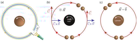
Figure 1.
(a) Sagnac effect in an optical loop around a spinning body (dragging of the ZAMOs): a “laboratory” observer, at rest with respect to the distant stars, sends light beams propagating in opposite directions along the loop; they take different times to complete the loop, the co-rotating one arriving first, by a time difference , Equation (7). (b) For particles in circular geodesics around a Kerr black hole, it is the other way around: the co-rotating one has the longer period. This is down to the combination of two oppositely competing effects: the dragging of the ZAMOs, tending to decrease the period of the co-rotating orbit vs. the gravitomagnetic force in Equation (9) (dragging of the compass of inertia), which is repulsive/attractive for co/counter-rotating orbits, thereby slowing/speeding up the orbit, respectively. The latter effect prevails, so that . (c) Around an infinite spinning cylinder of the Weyl class, ; hence, only the dragging of the ZAMOs subsists, and the situation for circular geodesics is opposite to (b) [thus similar to (a)]: the co-rotating geodesic has the shortest period, the difference reducing exactly to the Sagnac time delay, .
Consider now an axistationary spacetime, whose line element (1) simplifies to (in spherical-type coordinates)
In spite of being at rest, the laboratory observers (2) have, in general, non-zero angular momentum. The component of their angular momentum along the symmetry axis is, per unit mass [10,34,44],
which is zero iff . This manifests physically as follows. Take an observer at , and consider a circular optical loop (e.g., an optical fiber) of the same radius around the axis , see Figure 1a. Such an observer will measure a Sagnac effect; i.e., it will see light beams emitted in opposite directions along the loop not completing it at the same time, the difference in (coordinate) arrival times being, according to Equation (4),
Only observers with zero angular momentum (ZAMOs) measure no Sagnac effect. These observers are such that , i.e., have angular velocity
That the Sagnac effect vanishes for them can easily be seen by performing a local coordinate transformation , leading to a coordinate system where the ZAMO at is at rest. The metric form thereby obtained is diagonal at : , hence, . This singles out the ZAMOs as those who regard the directions as geometrically equivalent; for this reason, they are said to be those that do not rotate with respect to “the local spacetime geometry” [10].
If2 , the coordinate system in (5) corresponds to a rigid frame anchored to the asymptotic inertial frame at infinity (i.e., to the distant stars). Hence,
- •
- the “laboratory” observers, at rest in a frame fixed to the distant stars, have non-zero angular momentum (6) (measuring a Sagnac effect);
- •
- the zero angular momentum observers have non-zero angular velocity (8) in a coordinate system fixed to the distant stars (or as “viewed” from an observer at infinity).
These features are usually assigned to “frame-dragging”; we point out that it in fact consists of the dragging of the ZAMOs, and the gravitomagnetic object governing it is the potential 1-form (or equivalently, the gravitomagnetic vector potential ). These are the frame-dragging effects involved in arranging the bodies’ angular momentum/angular velocities in e.g., the black hole–ring and black hole–disk systems in [18,45], as well as in black saturn systems [17], as discussed in Section 3 and Figure 2 below.
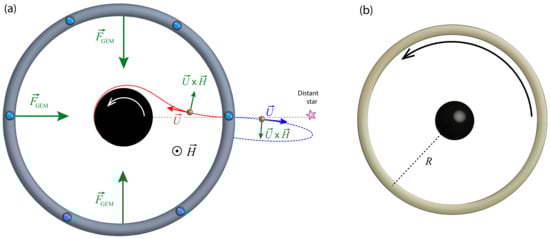
Figure 2.
(a) A space station (radius around a spinning Kerr black hole (). It is not “dragged” around: if initially static, it remains so, each hatch pointing to the same distant star. The dragging of the compass of inertia does not affect it: the gravitomagnetic (i.e., Coriolis) forces vanish, the gravitational forces (9) exerted on the station reducing to gravitoelectric (i.e., “Newtonian”) forces, , which are radial. It is affected only by the dragging of the ZAMOs, causing it to have a non-zero angular momentum, manifesting e.g., in a Sagnac effect along optical fiber loops around the station. A particle dropped from rest is deflected, along its infall, in the direction of the BH’s rotation, by the gravitomagnetic force ; however, a particle launched with initial outwards radial velocity ( for the blue dashed trajectory) is deflected in the opposite direction, contradicting again the naive body-dragging picture. [Red and blue dashed trajectories are plots in Boyer–Lindquist coordinates obtained by numerically solving the geodesic equation]. (b) A rotating ring around a ‘non-spinning’ BH. The BH does not acquire any angular acceleration, and the configuration remains stationary. The consequence of the ring’s rotation is (via the dragging of the ZAMOs) causing a zero angular momentum BH (; to have non-zero horizon angular velocity () and, conversely, a BH with zero angular velocity to have non-zero angular momentum.
2.2. Dragging of the Compass of Inertia: Gravitomagnetic Field and Lense-Thirring Effects
Consider a (point-like) test particle of worldline , 4-velocity and mass m. The space components of the geodesic equation yield3, for the line element (1) [26,27,31,32,33,34],
where is the Lorentz factor between and ,
is the Levi–Civita covariant derivative with respect to the spatial metric , with the corresponding Christoffel symbols, and
are vector fields living on the space manifold with metric , dubbed, respectively, “gravitoelectric” and “gravitomagnetic” fields. These play in Equation (9) roles analogous to those of the electric () and magnetic () fields in the Lorentz force equation, . The analogy also motivates dubbing “gravitomagnetic vector potential”. Here, denotes covariant differentiation with respect to the spatial metric [i.e., the Levi–Civita connection of ], Equation (10) is the standard 3-D covariant acceleration, and Equation (9) describes the acceleration of the curve obtained by projecting the time-like geodesic onto the space manifold , with as its tangent vector [identified in spacetime with the projection of onto : , see Equation (3)]. The physical interpretation of Equation (9) is that, from the point of view of the laboratory observers, the spatial trajectory will appear accelerated, as if acted upon by the fictitious force (standing here for “gravitoelectromagnetic” force4). In other words, the laboratory observers measure inertial forces, which arise from the fact that the laboratory frame is not inertial; in fact, and are identified in spacetime, respectively, with minus the acceleration and twice the vorticity of the laboratory observers:
They may be regarded as the relativistic generalization of, respectively, the Newtonian gravitational field and the classical Coriolis field, encompassing them as limiting cases [9]. It is that governs, via Equation (9), the Coriolis (i.e., gravitomagnetic) forces generated inside a spinning hollow sphere, noted by Einstein [1,46] and Thirring [2]; or those acting on test particles in the exterior field of a spinning body, causing the Lense–Thirring orbital precession [2,7]. It governs also the “precession” of gyroscopes with respect to the reference frame associated to the coordinate system in (1): according to the Mathisson–Papapetrou equations [24,47,48,49,50], under the Mathisson–Pirani spin condition [47,51], the spin vector of a gyroscope (i.e., a spinning pole-dipole particle) of 4-velocity is Fermi–Walker transported along its center of mass worldline ,
where . The spin vector is spatial with respect to , , and so, for a gyroscope whose center of mass is at rest in the coordinates of (1), [see Equation (2)], the space part of Equation (13) reads (using the Christoffel symbols in footnote, and noting that ) [28,31,32,34]
resembling the precession of a magnetic dipole in a magnetic field, . Likewise, the Sagnac time delay in an optical gyroscope (i.e., a small optical loop C) is also governed by the gravitomagnetic field , as can be seen by applying the Stokes theorem to (4), considering the surface with boundary ,
where , , is the Levi-Civita tensor of the space manifold , and the “area vector” of the loop (see [34] and footnote on p. 7 therein).
The gravito-electromagnetic analogy also extends to the field equations:
where the equations for and are, respectively, the time–time and time–space projections of the Einstein field equations , with and , and the equations for and follow directly from (11). They strongly resemble the Maxwell equations in a rotating frame; see Table 2 of [32].
Equation (13) tells us that the gyroscope’s axis is fixed with respect to a Fermi–Walker transported frame, which mathematically defines a locally non-rotating frame (e.g., [6,10]); it is said to follow the “compass of inertia” [6,7,32]. This agrees with the notion that gyroscopes are objects that oppose changes in the direction of their rotation axes. Hence, the gyroscope “precession” in (14) is thus in fact minus the angular velocity of rotation of the coordinate basis vectors relative to a locally non-rotating frame. Consider now the case that , in which the coordinate system in (1) corresponds to a rigid frame anchored to the asymptotic inertial frame at infinity. So, at infinity, the reference frame is inertial; however, at finite distance from the mass-energy currents that [by (17)] source , one has, in general, , and so that same rigid frame is rotating (besides being accelerated, as the observers at rest therein are not freely falling, ). One can thus say that the motion of the sources (or mass-energy currents, in general) drags the local inertial frames, or the local compass of inertia. In some literature, this is cast as the appearance of vorticity [52,53], the two notions being equivalent5 via Equation (12).
2.3. Competing Effects—Circular Geodesics
Let be the 4-velocity of a test particle moving along an equatorial circular geodesic in an axistationary spacetime (with reflection symmetry about the equatorial plane [54]), and the corresponding Lagrangian. The angular velocity of the circular geodesics is readily obtained from the Euler–Lagrange equations,
whose r-component yields, for ,
Its solution is
the + (−) sign corresponding, for and (i.e., attractive ), to prograde (retrograde) geodesics, i.e., positive (negative) directions. This equation tells us that, when depends on r, the periods of prograde and retrograde geodesics differ; this effect has been dubbed the gravitomagnetic “clock effect” [55,56,57,58]. The difference is given by
Using , noticing that reflection symmetry implies, in the equatorial plane, , we have, by (11), , and so (cf. [34])
Hence, the gravitomagnetic clock effect consists of the sum of two contributions originating from the two types of frame-dragging in Section 2.1 and Section 2.2: the Sagnac time delay (7) around the circular loop, due to the dragging of the ZAMOs, governed by , plus a term due to the gravitomagnetic (or Coriolis) forces generated by the dragging of the compass of inertia, governed by the gravitomagnetic field . The physical interpretation of the latter is as follows: for circular orbits, the gravitomagnetic force in Equation (9) is radial (since and ), being centrifugal or centripetal depending on the direction of the orbit, thus respectively decreasing or increasing the overall attraction, and, consequently, the velocity of the orbits. See Figure 1b.
It is important to notice that the two contributions in (20) are independent. In fact, there are solutions for which vanishes whilst is non-zero, as is the case of the Lewis metric of the Weyl class, describing the exterior gravitational field produced by infinitely long rotating cylinders. The metric is given, in star-fixed (“canonical”) coordinates, by Equation (61) of [34], yielding, in the form (1),
for . Here and j are, respectively, the Komar mass and angular momentum per unit length, and the parameter governing the angle deficit (, for a cylinder spinning in the positive direction). Trivially , hence and so
i.e., the difference in period between co- and counter-rotating circular geodesics equals precisely the Sagnac time delay for photons, the co-rotating one having a shorter period.
The two contributions can even be opposing, as is the case for the Kerr metric. We have, in this case, in the equatorial plane,
and so (observe that always6, in order for the counter-rotating orbit to exist)
i.e., the two contributions have opposite signs. Namely, the dragging of the ZAMOs tends to decrease the period of the orbit co-rotating with the black hole by , as compared to the counter-rotating orbit; however, the gravitomagnetic force (dragging the compass of inertia) does the opposite, tending to increase the period of the co-rotating orbit (case in which is repulsive), as compared to the counter-rotating orbit (case in which is attractive), by , see Figure 1b. Since , it is the gravitomagnetic force that prevails, making the co-rotating orbits slower overall than the counter-rotating ones.
The gravitomagnetic force and the corresponding have a close electromagnetic analogue in the magnetic force exerted on charged test particles orbiting a spinning charged body, see Equation (30) of [34]—only with a different sign, which manifests that (anti-) parallel mass/energy currents have a repulsive (attractive) gravitomagnetic interaction, as opposed to magnetism, where (anti-) parallel charge currents attract (repel) (see [59] and Section 13.6 of [60]).
2.4. Gravitomagnetic “Tidal” Effects: “Differential” Dragging and Force on Gyroscopes
A third class of frame-dragging effects that has been (more recently) discussed in the literature [19,61,62], distinct from those in Section 2.1 and Section 2.2, is the “differential precession” of gyroscopes. It consists of the precession of a gyroscope relative to a frame attached to the spin axes of guiding gyroscopes at a neighboring point. The effect was originally derived7 in [19]; we briefly re-derive it below in a straightforward manner, using Fermi coordinates.
The spin vector of a gyroscope in a gravitational field is Fermi–Walker-transported along its worldline, according to the Mathisson–Papapetrou–Pirani Equation (13). Consider an orthonormal tetrad Fermi–Walker-transported along the worldline of the set of gyroscopes 1. There is a coordinate system , rectangular at L, and adapted to such tetrad (), the so-called [64] “Fermi coordinates”, where the metric takes, to order , locally the form
(cf. e.g., Equation (18) in [65], setting therein ). Here, is the acceleration of the fiducial worldline , and are components of the curvature tensor evaluated along L. Let denote the coordinate basis vectors and its Christoffel symbols, . Along L, the vectors are Fermi–Walker-transported, so . Hence, gyroscopes moving along L (by definition), or momentarily at rest () at some event of L, do not precess relative to this frame, , by virtue of Equation (13). However, at some location outside L (), we have , and so the basis vectors are no longer Fermi–Walker-transported. That means that gyroscope 2, at the location , will precess with respect to this coordinate system. If the gyroscope is therein at rest (), we have
where, in the first equality, we noticed that , and, in the second, that , while only terms to first order in X are to be kept in (24) to the accuracy at hand. In the last equality, we noticed that , and that, by the definition of the coordinate system (see e.g., Figure 13.4 of [10]), are components of the vector at L tangent to the (unique) spatial geodesic emanating orthogonally from L and passing through the event , whose length equals that of the geodesic segment. It can be interpreted as the “separation vector” between and the simultaneous () event . Using the space projection relation (cf. Equation (5) in [32]) which, in the coordinate system (orthonormal at L), reads: , we have
where is the “gravitomagnetic tidal tensor” (or “magnetic” part of the Riemann tensor) as measured along L, and in the second equation, we noted that . Thus, is the angular velocity of precession of gyroscopes at location with respect to the Fermi frame locked to the guiding gyroscopes at the neighboring worldline L (of course, this is just minus the angular velocity of rotation of the basis vectors relative to Fermi–Walker transport). We can cast this effect as a “differential dragging” of the compass of inertia.
Another effect governed by the gravitomagnetic tidal tensor is the spin-curvature force exerted on a gyroscope, described by the Mathisson–Papapetrou equation [24,47,48,49,50]
where is the body’s spin tensor, and in the second equality, we employed the Mathisson–Pirani [47,51] spin condition , under which one can write . This force is of different nature from the inertial GEM “forces” in the geodesic Equation (9), in that it is a physical, covariant force, causing the body’s 4-momentum to change, and its motion to be non-geodesic, .
Both Equations (25) and (26) have exact (up to constant factors) electromagnetic analogues in terms of the magnetic tidal tensor [50,66], namely, the differential precession of magnetic dipoles () [67], and the force on a magnetic dipole [32,50,66].
Another manifestation is in the geodesic deviation equation (e.g., [7,10]). In vacuum, one can decompose the Riemann tensor in terms of the gravitoelectric and gravitomagnetic tidal tensors as measured by some laboratory observer , see decomposition (44) of [50]; hence, with respect to such an observer, the relative acceleration of nearby test particles (of 4-velocity ) comes in part from , which could thus be measured through gravity gradiometers [68].
Finally, observe that, around the origin of the Fermi coordinate system in (23), the gravitomagnetic field as given by Equation (12), , (which is generally valid, cf. Appendix A), reads
Moreover, in the coordinate system of the stationary metric (1), we have [32]
(for a — relation valid for orthonormal frames in arbitrary spacetimes; see Equation (110) of [32]). We can thus say that is essentially [to leading order, in the case of (27)] a derivative of the gravitomagnetic field . So, we can cast the different frame-dragging effects in the literature into the three levels of gravitomagnetism in Table 1, corresponding to three different orders of differentiation of the gravitomagnetic 1-form .

Table 1.
The different effects under the denomination “frame-dragging”, cast into three levels of gravitomagnetism, corresponding to different orders of differentiation of the gravitomagnetic vector potential .
We emphasize that these levels are independent: there exist solutions where only the first level () is intrinsically non-zero, as we have seen in Section 2.3; and others possessing the first two levels, but where the third vanishes. Examples of the latter are the Gödel universe and the uniform Som–Raychaudhuri metrics which, as discussed in detail in Section VII.B.3 of [69], are stationary solutions possessing zero gravitoelectric field () and non-zero uniform gravitomagnetic field , leading, by virtue of Equation (27), to vanish for the rest observers therein, whilst both and . In such metrics, by Equation (26), no force acts on gyroscopes at rest (whose worldlines are geodesic); and, by Equation (25), they moreover do not precess with respect to neighboring guiding gyroscopes.
3. Frame-Dragging Is Never “Draggy”8—No Body-Dragging
It is a widespread myth that when a massive body (e.g., a black hole) rotates, it drags everything around it. It seemingly originates from the fluid dragging analogy proposed originally in [5,36] and reinforced in [12,13], disseminating in the subsequent literature that the dragging of inertial frames can be explained in analogy with the dragging of a viscous fluid by an immersed rotating body. It is sometimes also portrayed as the whirlpool analogy [13,70]. Such mental pictures can be extremely misleading [22,37,70]; frame-dragging, in none of its levels, produces that type of effects. What are dragged are the ZAMOs, and the compass of inertia. The former leads to Sagnac and other akin global effects (having no local effect on the motion of test particles); the latter originates Coriolis (or gravitomagnetic) inertial forces on test particles. Such forces, however, affect only bodies moving with respect to the chosen reference frame, and are orthogonal to the body’s velocity; hence, never of the viscous/dragging type. This later aspect was stressed in an illuminating paper by Rindler [37], based on linearized theory, in the framework of a weak field and slow motion approximation.
Rindler’s conclusion can be readily generalized to the exact theory using Equation (9) [for stationary spacetimes, or with Equation (A2) of Appendix A for arbitrary fields]. Imagine that an advanced civilization builds a circular space station around a Kerr black hole, as illustrated in Figure 2a, and imagine that it is initially set fixed with respect to the distant stars (which can be set up by pointing a telescope to a distant star). Regardless of the black hole’s rotation, the station will not be dragged into any rotational motion: since, initially, , by Equation (9) the only inertial force (per unit mass) acting on any of its mass elements is the radial force produced by the gravitoelectric field (i.e., by the relativistic generalization of the Newtonian field): ; this force is counteracted by the stresses in the station’s structure (which prevent it from collapsing), and so for all mass elements at all times. That is, the station remains static, with, e.g., its hatches pointing to the same fixed stars. It is, in particular, unaffected by the dragging of the compass of inertia. The situation is only distinct from that around a static black hole in that here the station’s angular momentum per unit mass in non-zero [cf. Equation (6)],
implying, e.g., that a Sagnac effect will be measured in an optical fiber loop along the station; see Section 2.1 and Figure 1a [the difference in arrival times for beams propagating in opposite directions along the station being given by in (22), making therein ]. It implies also that it is impossible for the crew members along the station to all have their clocks synchronized (see, e.g., [34] Sections 5.3.2–5.3.3).
Imagine now that a crew member starts throwing objects (test particles); by having a non-zero velocity () with respect to the star-fixed reference frame, gravitomagnetic (i.e., Coriolis) forces will now act on them, cf. Equation (9). The gravitomagnetic field in the equatorial plane of the Kerr spacetime is given by Equation (21); it is orthogonal to the plane, pointing up. Consider, in particular, as depicted in Figure 2a, one test particle dropped from rest from the station, and another one launched with an initial outwards radial velocity. The in-falling particle is indeed deflected in the direction of the black hole’s rotation; however, the outgoing one is deflected in the opposite direction, contradicting the naive fluid dragging picture. This exemplifies how different Coriolis forces are from viscous dragging-type forces. In other words, the dragging of the compass of inertia is a phenomenon very different from “body-dragging.”
Another example of this difference is provided by the circular geodesics around the black hole, depicted in Figure 1b: the orbits are stationary; their motion is not accelerated/decelerated by the black hole’s rotation (as would be the case if there were some viscous coupling). The Coriolis forces are in this case radial, consequently just changing the overall gravitational attraction. Since they are repulsive (attractive) for co-(counter-) rotating orbits, their effect is to actually (for a fixed radius r) make the co-rotating geodesic slower than the counter-rotating one, somewhat at odds with the naive dragging picture, as pointed out in [22,70,71].
It is also instructive to consider the reciprocal of the setting in Figure 2a, i.e., a non-spinning black-hole perturbed by a rotating ring or disk around it. The gravitational field produced by such setting is given by the perturbative treatments in [45] (for a ring), and in [18] (for a disk perturbing a Schwarzschild black hole). Again, regardless of the ring/disk’s rotating motion, the black hole is not dragged around, in the sense of acquiring any “angular acceleration”. In fact, these solutions are stationary. The impact of ring/disk’s rotation is (via the dragging of the ZAMOs) causing a black hole with zero angular momentum to have a non-zero horizon angular velocity [18,45,72] and, conversely, a non-rotating black hole to have a non-zero angular momentum [45,72]—thereby even introducing a certain ambiguity in a black hole’s spinning/non-spinning character. Let us see this in detail. First observe that , and so the ZAMOs are orthogonal to the hypersurfaces of constant time t, i.e., such hypersurfaces are their rest spaces. We can thus say that, at each point, these hypersurfaces are rotating, with respect to Boyer–Lindquist coordinates (anchored to inertial observers at infinity) with an angular velocity , cf. Equation (8) (also called the “dragging angular velocity” e.g., [18]). The horizon is a 2-surface embedded in a hypersurface of constant t, having the special property that therein becomes independent9 of ; so, the horizon rotates rigidly with angular velocity , sometimes dubbed the “black hole’s angular velocity” [10,74,75]. The black hole’s angular momentum is given [18,45,76] by the Komar integral associated with the axisymmetry Killing vector field : , for some 2-surface enclosing the black hole but not the ring (in the case of the disk, is the BH horizon). The ring’s angular momentum is , for enclosing the whole system. For a BH-ring system, when the BH’s angular momentum is zero (), the horizon angular velocity is non-zero, and given by Equations (75) and (68) of [45],
where R is the ring’s circumferential radius. Conversely, when the horizon’s angular velocity is zero (), the BH’s angular momentum is non-zero (negative):
where is the horizon’s area, cf. Equations (76), (68), and (26) of [45].
It is also worth mentioning that entirely analogous conclusions to the above can be drawn using “black saturns” [17], which are exact (4 + 1)-dimensional solutions describing a black hole surrounded by a black ring.
3.1. Test Particles in Static Equilibrium around Spinning Black Holes
Perhaps the sharpest counter-examples to the notion of body-dragging, and how drastically actual frame-dragging (in any of its levels) differs from it, is the existence of static equilibrium positions for test particles around some spinning black hole spacetimes, such as the Kerr-de Sitter and (for charged particles) the Kerr–Newman spacetimes. The metrics of both these spacetimes are encompassed in the line element (Kerr–Newman–dS metric [77])
where is the cosmological constant, and Q the black hole’s charge.
3.1.1. Kerr-de Sitter Spacetime
This metric is obtained by setting in (28)–(30). The gravitoelectric field [i.e., minus the acceleration of the laboratory observers, Equation (12)] is, in the equatorial plane (),
It vanishes at (“static radius” [78]), where the cosmological repulsion exactly balances the gravitational attraction. By virtue of Equation (9), this means that no gravitational inertial force is exerted on a particle at rest at , ; i.e., particles placed there remain static (), while following a geodesic worldline (). They are not dragged in any way by the black hole’s rotation, no tangential force being needed to hold them in place, unlike one might think based on the viscous fluid dragging analogy. Frame-dragging has no detectable effect on such particles, only causing them (via the dragging of the ZAMOs) to have non-zero angular momentum,
3.1.2. Kerr–Newman Spacetime
An analogous situation occurs in the Kerr–Newman spacetime, in this case for charged particles. This metric is obtained by setting in (28)–(30); the corresponding electromagnetic 4-potential 1-form is . Consider now a (point-like) test particle of 4-velocity , mass m, and charge q. Its equation of motion is , whose space part, in the “laboratory frame”, reads, cf. Equations (9) and (A7),
where and denote, respectively, the space components of the electric field and magnetic field as measured by the laboratory observers (2). In the equatorial plane, and read
The equilibrium positions are given by the condition ; noticing that [cf. Equation (2), and recall that ], this condition becomes (in the equatorial plane)
which, in the non-naked scenario , and outside the ergosphere, , yields the single solution [79]
with Q and q having the same sign (as expected), and . Hence, a particle with such a charge, placed at , remains at rest, with no gravitomagnetic nor magnetic force acting on it since .
3.2. “Bobbings” in Binary Systems
Frame-dragging plays a crucial role in the dynamics of binary systems. Among other effects, it is at the origin of the bobbings observed in numerical simulations [80,81] of nearly identical black holes with anti-parallel spins along the orbital plane (“extreme kick configurations”, see Figure 3 and Figure 4), in which the whole binary (i.e., its center of mass) oscillates “up and down.” They are an example of a setting where the naive viscous fluid analogy, and its associated “body-dragging” misconception, lead to predictions opposite to the real effects.
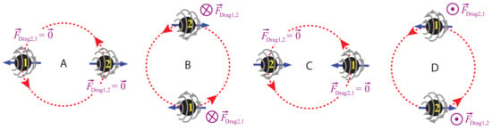
Figure 3.
Incorrect prediction of the bobbing motions of “extreme kick” spinning black hole binaries, as would follow from the body-dragging misconception (illustration based on Figure 5 of [82]). Each black hole would be acted by a viscous-type dragging force () originated by the spin of the other black hole; such forces would vanish when the black holes’ spins lie along the axis connecting them (phases A and C), and be maximum when the spins are orthogonal to such an axis (phases B and D), each black hole dragging the other inwards of the plane of the illustration in phase B, and outwards in phase D. None of these forces exist, however.
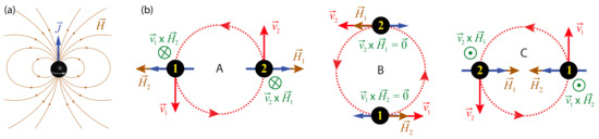
Figure 4.
(a) The field lines of the gravitomagnetic field produced by a spinning black hole (of spin vector ); it is similar (far from the BH) to that of a magnetic dipole oriented oppositely to . (b) The actual picture of the corresponding spin-orbit gravitomagnetic forces involved in the bobbing motion, with phase D suppressed, since the result is similar to B. The situation is opposite to that in Figure 3: the forces vanish when the spins are orthogonal to the axis connecting the black holes (phases B and D, as therein , ), and have maximum magnitude when they lie along such an axis, pushing the pair out of the plane of the illustration in phase A, and inwards in phase C.
The setting is illustrated in Figure 3; according to the fluid dragging analogy, in phases A and C, there would be no dragging forces, which would be maximum in B and D, each black hole dragging the other into the plane of the illustration in phase B, and outwards in phase D. None of this is true, however.
The gravitomagnetic field of a body (or black hole) with spin vector is given, at leading order, and in its post-Newtonian (PN) rest frame, by (e.g., [7,9])
similar to that of a magnetic dipole, with in the place of the magnetic moment . Its field lines are depicted in Figure 4a. The gravitomagnetic force exerted by black hole 1 (BH 1) on black hole 2 (BH 2) is, in the former’s PN instantaneous rest frame, , where is the velocity of BH 2 relative to BH 1, and in the last equality, we used , and approximated . Using the vector identity (5.2a) of [83], it reads
where is the position vector of BH 2 relative to BH 1, and in the second equality, we noticed that , since the black hole’s spins lie in the orbital plane, and for quasi-circular motion. The analogous expression for follows by interchanging in (32). It is clear from Figure 4 that these forces vanish in phases B and D, as therein the BHs’ velocities are aligned with their gravitomagnetic fields: , . They have maximum magnitude in phases A and C, when each black hole’s velocity is orthogonal to the other’s spin-vector, pointing out of the plane of the illustration in phase A, and inwards in phase C. That is, the situation is opposite in phasing to the “body-dragging” picture of Figure 3. (It is rather surprising that in [84], where Figure 3 is reproduced, and at the same time equations equivalent to the above are presented, this disagreement has seemingly gone unnoticed).
The Origin of the Bobbing
The gravitomagnetic forces ( and ) each black hole exerts on the other, which are spin-orbit interactions, point in the same direction, seemingly causing the whole pair to accelerate. Albeit true, it is not the whole story, as these are not the only spin-orbit forces in this system. Each black hole also exerts a spin-curvature force given by Equation (26), which is of the same order of magnitude [albeit of different nature; not an inertial force but a “real”, covariant force, causing the body to deviate from geodesic motion, as discussed in Section 2.4], as we shall now see.
Compact bodies such as black holes have angular momentum , hence the gravitomagnetic acceleration in Equation (32) is of the order , i.e., it arises at 1.5 order in the post-Newtonian (PN) expansion, see Appendix A.1. Thus, we need equations of motion for spinning (pole-dipole) bodies accurate to 1.5 PN order. These follow by taking the 1.5 PN limit of the Mathisson–Papapetrou Equation (26), which reduces (see Appendix A.3) to (A8), with the 1.5PN limit of the spin-curvature force . The force exerted by BH 2 on BH 1 is , where is the gravitomagnetic tidal tensor produced by BH 2 as “measured” by BH 1 (Equations (88)–(89) and (94) in [50]); it reads [50,85,86,87]
where, again, in the second equality, we noticed that for spins lying in the orbital plane, that for quasi-circular motion, and that . The analogous expression for follows by interchanging in (33). Observe that it is (not ) which should be regarded (in the context of a PN approximation) as the “reaction” to the gravitomagnetic force in Equation (32), as these are the ones that depend on ; and note that they do not cancel out:
That is, the spin–orbit interactions do not obey an action–reaction law [87]. It is this mismatch that causes the whole binary to bob. Consider the PN frame momentarily comoving with BH 1; the 1.5PN gravitational field generated by BH 1 is, in such a frame, described by the metric (A3) in Appendix A.1,
with w given by Equation (A11) with , and , , cf. Equations (A12). The equation of motion for BH 2 is then, by Equation (A8),
with [cf. Equation (A15) with ]. The extreme kick configuration corresponds to the case that , ; hence, , cf. Equation (32). Since and lie both in the orbital plane , by (35) the z-coordinate acceleration of BH 2 reduces to
where , v is the magnitude of the BH’s velocities with respect to the binary’s center of mass frame, , and in the last equality, we assumed (without loss of generality) the system to be at phase A of Figure 4 at . By analogous steps, one finds the same z-coordinate acceleration for BH 1, ; that is, the bobbing is synchronous, the whole binary (thus its center of mass) oscillating up and down.
It should be stressed that such bobbing, and the mismatch between action and reaction in the spin-orbit forces, do not imply a violation of any conservation principle; on the contrary, as shown in [84], it is a necessary consequence of the interchange between mechanical momentum of the bodies and field momentum (in the sense of the Landau–Lifshitz pseudotensor [88]).
It should also be remarked that, in Ref. [82], where the scheme in Figure 3 was originally presented, still the author was remarkably not misled into a qualitatively wrong phasing. Therein a notion of “space dragging”, seemingly different from a viscous fluid analogy, and seemingly imparting a maximum bobbing velocity at stages B and D is used (hence apparently closer to the phenomena involved in the ZAMOs dragging, as if each black hole was “trying” to maintain constant its orbital angular momentum about the other). Such a notion agrees in phasing with Equation (36), which, integrating, yields : it is indeed in phases B and D ( and , respectively) that the bobbing velocities have maximum magnitude. However, we notice that, as discussed in Section 2, the gravitomagnetic forces (dragging of the compass of inertia) are actually of different origin from the ZAMOs dragging; and that such a notion is, at best, complicated and much less intuitive than the gravitomagnetic picture.
Finally, we made use above of a PN frame momentarily comoving with BH 1, which greatly simplified computations, since, in this case: the gravitomagnetic field produced by BH 1 reduces to that generated by its spin, Equation (31); the gravitomagnetic force encodes the whole spin-orbit inertial force acting on BH 2, and lies along . In other PN frames (such as one momentarily comoving with the binary’s center of mass, as depicted in Figure 3 and Figure 4), the description is more complicated, as then includes a contribution due to BH 1’s translational motion, Equation (A16), and part of the spin-orbit inertial force is then encoded in the gravitoelectric field [having then a non-vanishing z-component, see Equation (A15)]; however, the total spin-orbit inertial force is the same, and equal to (32). Likewise, the spin-curvature force does not depend on the chosen PN frame, so neither does the z-coordinate acceleration, which holds for a generic PN frame, cf. Equation (A20). The derivation for a generic PN frame is given in Appendix A.3.
4. Conclusions
Generically very feeble in the solar system, where they have been subject of different experimental tests [89,90,91,92,93,94,95,96] (including dedicated space missions [91,95], as well as some controversies [97,98,99,100]), gravitomagnetic effects become preponderant in the strong field regime, shaping the orbits of binary systems and the waveforms of the emitted gravitational radiation [101,102,103,104,105]. Yet, they are still commonly misunderstood; in particular, those dubbed “frame-dragging”. Pertaining initially to the dragging of the compass of inertia, the usage of the term has been extended to other gravitomagnetic effects, as well as to persistent misconceptions fueled by the deceptive fluid-dragging analogy—possibly even by the very term “dragging”. We aimed in this paper to deconstruct such misconceptions, explaining what the different types of frame-dragging effects consist of, and the relationship between them. We split them into three different levels (Table 1), governed by three distinct mathematical objects, corresponding to different orders of differentiation of the gravitomagnetic potential 1-form . The first level (Section 2.1), governed by itself, may be cast physically (in axistationary spacetimes) as the dragging of the ZAMOs, which comprises effects such as the Sagnac effect in optical loops around the source, or the arrangement of the bodies’ angular velocities/angular momentum in black holes surrounded by disks or rings (Section 3). It contributes also to the gravitomagnetic clock effect (Section 2.3). The second level, governed by the gravitomagnetic field , and physically interpreted as the dragging of the compass of inertia (Section 2.2), includes the gravitomagnetic (or Coriolis) forces on test bodies and the Lense–Thirring orbital precessions, gyroscope precession, and is also responsible for the remainder of the gravitomagnetic clock effect. The third level (Section 2.4), governed by the gravitomagnetic tidal tensor (“magnetic” part of the Riemann tensor), and interpreted as a differential dragging of the compass of inertia, physically manifests in the relative precession of nearby sets of gyroscopes, and in the spin-curvature force on a gyroscope. These levels are largely independent, in that there exist spacetimes possessing only the first (which we exemplified with spinning Lewis-Weyl cylinders, Section 2.3), and others possessing only the first two levels, but missing the third (e.g., the Gödel universe). In the case of the first two levels (dragging of the ZAMOs vs dragging of the compass of inertia), their effects can actually be opposite, as exemplified here by the case of circular geodesics in the Kerr spacetime (Section 2.3).
Two main analogies are commonly used to help to physically interpret the frame-dragging effects: the analogy with magnetism (which created the term “gravitomagnetism”) and the fluid dragging analogy. The former is clearly useful for the second and third levels of frame-dragging, since not only the gravitational effects comprised therein have an electromagnetic analogue, as the exact equations describing them exhibit, in the appropriate formalism, exact analogies (up to constant factors) with the electromagnetic counterparts (Section 2.2, Section 2.3 and Section 2.4). As for the first level, they have no analogue in classical electromagnetism (only in quantum electrodynamics10). The fluid model, on the other hand, draws an analogy with the dragging of a viscous fluid by a moving/rotating body. It gives some qualitative intuition (in a loose sense) for the first level of frame-dragging, in that in all the systems considered herein (black hole spacetimes, and infinite spinning cylinders) the ZAMOs are dragged in the same direction of the source’s rotation. The parallelism ends there however: other features of any fluid flow, such as the unavoidable dragging of immersed bodies along with the flow, have no parallel in any of the frame-dragging levels. The dragging of the compass of inertia, in particular (which was the original motivation for such analogy), is a very different (sometimes opposite, cf. Section 3 and Section 3.2) phenomenon from body-dragging. Some of these inconsistencies have been pointed out in the literature, namely in a paper by Rindler [37]—based, however, on a weak field slow motion linearized theory approach, the question remaining as to whether the conclusions would fully hold in the exact case. We generalized them here (Section 3) to the exact theory, using the exact 1 + 3 GEM formalism. We considered first (as an application akin, on the whole, to [37]) a space station around a spinning black hole (seen to remain stationary, without acquiring any rotation), as well as the situation for test particles launched from it, where those with initial outwards radial velocity are deflected in the direction opposite to the black hole’s rotation. We considered also the reciprocal problem—a rotating ring around a ‘non-spinning’ black hole (either with zero angular momentum, or zero horizon angular velocity), pointing out that the black hole acquires no angular acceleration of any sort, the solutions being stationary. As a very physical, and perhaps sharpest example to convince the reader that the (all too common) notion of “body-dragging” is wrong, and its underlying viscous fluid-dragging analogy extremely misleading, we considered equilibrium positions for test particles in spinning black hole solutions (namely Kerr–Newman and Kerr-de Sitter). Finally, we considered a notable phenomenon which is driven by frame-dragging—the bobbings in “extreme kick” binary systems—and where the viscous-dragging picture predicts the exact opposite of the real effect.
Author Contributions
Conceptualization, L.F.O.C. and J.N.; investigation, L.F.O.C. and J.N.; writing—original draft preparation, L.F.O.C.; writing—review and editing, L.F.O.C. and J.N. All authors have read and agreed to the published version of the manuscript.
Funding
L.F.C. and J.N. were supported by FCT/Portugal through projects UIDB/MAT/04459/2020 and UIDP/MAT/04459/2020.
Institutional Review Board Statement
Not applicable.
Informed Consent Statement
Not applicable.
Data Availability Statement
Not applicable.
Conflicts of Interest
The authors declare no conflict of interest. The funders had no role in the design of the study; in the collection, analyses, or interpretation of data; in the writing of the manuscript, or in the decision to publish the results.
Appendix A. Inertial Forces—General Formulation
The exact formulation of the inertial GEM fields given in Section 2.2, and, in particular, Equations (9)–(11), hold for stationary fields. We briefly present here its generalization for arbitrary fields. Several such formulations have been given in e.g., [28,29,30,32,35,106]; we will follow the exact approach in [32], which, in the corresponding limits, leads directly to the GEM fields usually defined in post-Newtonian approximations, e.g., [20,25,94], and (up to constant factors and sign conventions) in the linearized theory approximations, e.g., [7,21,22,23,24].
Consider a congruence of observers of 4-velocity , and a (point-like) test particle of worldline and 4-velocity . Let be the spatial projection of the particle’s velocity with respect to , cf. Equation (3); it yields, up to a () factor, the relative velocity of the particle with respect to the observers (cf. e.g., [28,50,63]). It is the variation of along that one casts as inertial forces (per unit mass); the precise definition of such variation involves some subtleties, however. For that, we need a connection (i.e., a covariant derivative) for spatial vectors that (i) in the directions orthogonal to should equal the projected Levi–Civita spacetime connection: , for any and orthogonal to , so that it corrects for the trivial variation of the spatial axes in the directions orthogonal to (for instance, of a non-rectangular coordinate system in flat spacetime) which is not related to inertial forces and does not vanish in an inertial frame; (ii) along the congruence, becomes an ordinary time-derivative , so that it yields the variation of with respect to a system of spatial axes undergoing a transport law specific to the chosen reference frame. The most natural of such choices is spatial axes co-rotating with the observers (“congruence adapted” frame [32]; arguably, the closest generalization of the Newtonian concept of reference frame [6,29]). For an orthonormal basis , whose general transport law along the observer congruence can be written as (e.g., [10,32])
that amounts to choosing (the angular velocity of rotation of the spatial axes relative to Fermi–Walker transport) equal to the observer’s vorticity: , as defined in (12). If the congruence is rigid, this ensures that the axes point to fixed neighboring observers. The connection that yields the variation of a spatial vector with respect to such a frame is , cf. Equation (51) of [32]; and the inertial or “gravitoelectromagnetic” force on a test particle as measured in such frame is the variation of along with respect to , that is, . Since, for geodesic motion, , it follows, using (3), that , where . Finally, from the decomposition (e.g., Equation (135) of [69])
where and are, respectively, the congruence’s shear and expansion, we have (using ) [32]
where the “gravitoelectric” and “gravitomagnetic” fields are again given by Equations (12) (being, respectively, minus the observers’ acceleration, and twice their vorticity), and m is the particle’s mass. For a congruence of observers (2) tangent to a time-like Killing vector field in a stationary spacetime (or for any rigid congruence of observers in general), , and so Equation (A2) reduces to Equation (9).
Appendix A.1. Post-Newtonian Approximation
The post-Newtonian expansion is a weak field and slow motion approximation tailored to bound astrophysical systems. It can be cast in different, equivalent ways; here, following [10,69,87,88,107,108], we frame the expansion in terms of a small dimensionless parameter , such that , where U is minus the Newtonian potential [i.e., taking the Newtonian limit of Equation (1), ], and the bodies’ velocities are assumed such that (since, for bounded orbits, ). In terms of “forces,” the Newtonian force is taken to be of zeroth PN order [0PN, i.e., ], and each factor amounts to a unit increase of the PN order. Time derivatives increase the degree of smallness of a quantity by a factor ; for example, . The 1PN expansion consists of keeping terms up to in the equations of motion [107]. This amounts to retaining terms up to in , in , and in , effectively considering a metric of the form [20,88]
(actually accurate to 1.5PN), where w consists of the sum of U plus non-linear terms of order , . For observers (2) at rest in a given coordinate system, by (12) , ; hence11
(cf. e.g., Equation (3.21) of [20]). Moreover, , , , , and thus Equation (A2) becomes
In terms of coordinate acceleration, noting that , , we have
(cf. Equation (7.17) of [20]), where stands for “post-Newtonian inertial force” (in order to distinguish from ). The absence of terms means that (A5) and (A6) are actually accurate to 1.5PN order.
“Linear dragging”.—The contribution to in (A4) (and thus to ) means that a time-varying gravitomagnetic vector potential induces a velocity-independent inertial force on a test particle. For instance, in the interior of an accelerating massive shell, inertial forces are induced in the same direction of the shell’s acceleration, as first noted by Einstein ([109], pp. 100–102; see also [110,111]). The effect has been studied in the framework of the exact theory in some special solutions (e.g., [112,113]), and has been experimentally confirmed to high accuracy (albeit indirectly, one may argue) in the observations of binary pulsars [114]. It is sometimes dubbed “translational dragging” [111] or “linear dragging” [112,115] (of inertial frames). We note that, in spite of such denominations, it is a component of the gravitoelectric field ; as such, in the given reference frame, it does not directly fit into the frame-dragging types in Table 1. It mixes, however, with the gravitomagnetic inertial acceleration (dragging of the compass of inertia) in changes of frame; for instance, as exemplified in Section 3.2 and Appendix A.3.1, an inertial force which, in a given PN frame, consists solely of the gravitomagnetic term , in another frame can be partially incorporated in the term (this stems from the transformation laws for and , which exhibit a certain analogy with their electromagnetic counterparts, see [108]).
Appendix A.2. Non-Geodesic Motion
When the test body is acted upon by a covariant force , and in the special case that (no “hidden momentum”) with the body’s rest mass m constant, then Equation (A2) is readily generalized to
and its post-Newtonian limit to
Appendix A.3. Equations of Motion for Spinning Binaries
Consider a system of isolated spinning pole-dipole bodies interacting gravitationally. Each body K is considered under the influence of the gravitational field “external” [20,86] to it, described (in the harmonic gauge in [20,25,86,88,94]), by the metric (A3) with [86,88]
accurate to 1.5PN order. Here , , is the point of observation, is the instantaneous position of body “A”, and its velocity. To this accuracy, is to be taken in expression (A9) as the Newtonian “acceleration” caused by the other bodies, .
The equation of motion for body 2 is the 1.5 PN limit of the Mathisson–Papapetrou Equation (26). Under the Mathisson–Pirani spin condition employed in (26), and, to the accuracy at hand, one can take (see [116]), hence (consistent also, to the accuracy at hand, with the Tulczyjew–Dixon and Ohashi–Kyrian–Semerák spin conditions; see [116,117,118] and Section 3.1 of the Supplement in [50]), leading, by Equation (A8), to
with the inertial force given by Equations (A4), (A6), and (A11)–(A12), and the 1.5PN limit of the spin-curvature force exerted by body 1 on body 2, , where is the gravitomagnetic tidal tensor produced by body 1 as “measured” by body 2 (Equations (88)–(89) and (94) in [50]). The latter force reads
(cf. [50,85,86,87]), where , and .
Appendix A.3.1. Extreme Kick Configuration
In this configuration, the bodies are assumed to be two black holes with approximately equal masses , and spins equal in magnitude but anti-parallel, , lying in the orbital plane . They are also assumed in a nearly circular orbit about the binary’s center of mass. In this case, and (similar relations holding for or in the place of , and ) and so Equation (A14) reduces to . By Equations (A4), (A11)–(A12), the gravitoelectric and gravitomagnetic fields as “seen” by BH 2 are
where we noticed that, at BH 2’s position (), . The last term of tells us that, in a generic reference frame, due to the translational motion of the source (BH 1), part of the spin-orbit inertial force is incorporated in the gravitoelectric field. Equation (A16) tells us that, in addition to the term due to BH 1’s spin, there is also the translational contribution to the gravitomagnetic field produced by BH 1. The gravitomagnetic force exerted on BH 2 reads
where in , we again used the vector identity (5.2a) of [83]. Since , the last two terms of in (A6) both vanish at BH 2’s position: ; The equation of motion for BH 2 is thus, by (A13),
with , and given by Equations (A15), (A17), and (A14). Splitting the PN inertial force into “monopole” and spin-orbit parts, , we can re-write
Hence, matches the gravitomagnetic force (32) exerted on BH 2, as measured in the PN frame momentarily comoving with BH 1, obtained in Section 3.2. That is: in a generic frame, the gravitomagnetic force does not encode the whole spin-orbit inertial force, part of it being encoded in the gravitoelectric force ; however, the total spin-orbit inertial force is the same in all PN frames. Since , we have, for the z- coordinate,
matching the result (36) obtained in Section 3.2.
Notes
| 1 | The future-pointing condition is , where is the vector tangent to the photon’s worldline. |
| 2 | Actually, the weaker condition that the congruence of observers at rest (2) is inertial at infinity suffices. |
| 3 | Computing the Christoffel symbols , , and , where . |
| 4 | In [32] a different convention was used, in that (and the term “inertial force”) therein actually refers to the inertial force per unit mass (i.e., the inertial “acceleration” , in the notation herein). |
| 5 | Indeed, the vorticity of a congruence of observers corresponds precisely to the angular velocity of rotation of the connecting vectors between neighboring observers with respect to axes Fermi–Walker transported, see e.g., footnote in p. 7 of [34]. |
| 6 | The innermost circular geodesics, in each direction, are the photon orbits whose radius is [16], and so . |
| 7 | In a perhaps less straightforward manner though, and with unnecessary restrictions. Namely, in [19], it is assumed that (besides being momentary comoving) the gyroscopes at L and have the same acceleration. This is not necessary, as shown here; in order for (25) to hold, one needs only , i.e., that gyroscope 2 has momentarily zero “Fermi relative velocity” [63] with respect to gyroscopes at L. Moreover, the results therein hold only for vacuum, as the magnetic part of the Weyl tensor is used instead of . |
| 8 | Inspired on the title of the session PT5
— “Dragging is never draggy: MAss and CHarge flows
in GR” (where “draggy”
had however no such meaning), held at the sixteenth Marcel Grossmann
Meeting (MG16), July 5-10 2021. |
| 9 | In any stationary black hole spacetime whose matter content obeys the weak energy condition and hyperbolic equations, the horizon is orthogonal to a (null) Killing vector field, i.e., it is a “Killing horizon” (see [73,74] theorem 2.2). |
| 10 | Namely the analogy between the Sagnac and the Aharonov–Bohm effects (see e.g., [34,35] and references therein); it does not, however, assist much in the understanding of the former, as the latter effect is, conceptually, more difficult. |
| 11 | For the expressions for the Christoffel symbols, see e.g., Equations (8.15) of [25], identifying , in the notation therein. |
References
- Einstein, A. Letter to E. Mach, Zurich, 25 June 1913; Freeman: San Francisco, CA, USA, 1973; see Ref. 10, page 544 (Figure 21.5). [Google Scholar]
- Mashhoon, B.; Hehl, F.W.; Theiss, D.S. On the Gravitational effects of rotating masses - The Thirring-Lense Papers. Gen. Rel. Gravit. 1984, 16, 711–750. [Google Scholar] [CrossRef]
- Cohen, J. Dragging of inertial frames by rotating masses. In Lectures in applied Mathematics, Relativity Theory and Astrophysics, 1. Relativity and Cosmology; American Mathematical Society: Providence, RI, USA, 1965; Volume VIII, pp. 200–202. [Google Scholar]
- Pugh, G.E. Proposal for a Satellite test of the Coriolis predictions of General Relativity. In Nonlinear Gravitodynamics—The Lense-Thirring Effect (2003); Ruffini, R., Sigismondi, C., Eds.; World Scientific: London, UK, 1959; pp. 414–426. [Google Scholar] [CrossRef]
- Schiff, L.I. Motion of a gyroscope according to Einstein’s theory of gravitation. Proc. Natl. Acad. Sci. USA 1960, 46, 871–882. [Google Scholar] [CrossRef] [PubMed]
- Massa, E.; Zordan, C. Relative kinematics in general relativity the Thomas and Fokker precessions. Meccanica 1975, 10, 27–31. [Google Scholar] [CrossRef]
- Ciufolini, I.; Wheeler, J.A. Gravitation and Inertia; Princeton Series in Physics: Princeton, NJ, USA, 1995. [Google Scholar]
- Gödel, K. Lecture on Rotating Universes. In Kurt Gödel Collected Works Volume III; Feferman, S., Ed.; Oxford U. P.: Oxford, UK, 1995; pp. 269–289. [Google Scholar]
- Costa, L.F.; Natário, J. The Coriolis field. Am. J. Phys. 2016, 84, 388. [Google Scholar] [CrossRef]
- Misner, C.W.; Thorne, K.S.; Wheeler, J.A. Gravitation; W. H. Freeman: San Francisco, CA, USA, 1973. [Google Scholar]
- Ciufolini, I. Dragging of inertial frames. Nature 2007, 449, 41–47. [Google Scholar] [CrossRef]
- Thorne, K.S. Relativistic Stars, Black Holes, and Gravitational Waves. In General Relativity and Cosmology, Proceedings of the International School of Physics “Enrico Fermi”, Course_47, Varenna, Italy, 30 June–12 July 1971; Academic Press: New York, NY, USA, 1971; pp. 237–283. [Google Scholar]
- Thorne, K.S.; Price, R.H.; Macdonald, D.A. (Eds.) Black Holes: The Membrane Paradigm; Yale University Press: New Haven, UK, 1986. [Google Scholar]
- Thorne, K.S. Gravitomagnetism, jets in quasars, and the Stanford Gyroscope Experiment. In Near Zero: New Frontiers of Physics; Fairbank, J.D., Deaver, B.S.J., Everitt, C.W.F., Michelson, P.F., Eds.; W. H. Freeman and Company: New York, NY, USA, 1988; pp. 573–586. [Google Scholar]
- Schaefer, G. Gravitomagnetic effects. Gen. Rel. Gravit. 2004, 36, 2223. [Google Scholar] [CrossRef]
- Bardeen, J.M.; Press, W.H.; Teukolsky, S.A. Rotating Black Holes: Locally Nonrotating Frames, Energy Extraction, and Scalar Synchrotron Radiation. Astrophys. J. 1972, 178, 347–370. [Google Scholar] [CrossRef]
- Elvang, H.; Figueras, P. Black saturn. J. High Energy Phys. 2007, 2007, 050. [Google Scholar] [CrossRef]
- Čížek, P.; Semerák, O. Perturbation of a Schwarzschild Black Hole Due to a Rotating Thin Disk. Astrophys. J. Suppl. Ser. 2017, 232, 14. [Google Scholar] [CrossRef]
- Nichols, D.A.; Owen, R.; Zhang, F.; Zimmerman, A.; Brink, J.; Chen, Y.; Kaplan, J.D.; Lovelace, G.; Matthews, K.D.; Scheel, M.A.; et al. Visualizing Spacetime Curvature via Frame-Drag Vortexes and Tidal Tendexes I. General Theory and Weak-Gravity Applications. Phys. Rev. D 2011, 84, 124014. [Google Scholar] [CrossRef]
- Damour, T.; Soffel, M.; Xu, C.M. General relativistic celestial mechanics. 1. Method and definition of reference systems. Phys. Rev. D 1991, 43, 3272–3307. [Google Scholar] [CrossRef]
- Harris, S. Conformally stationary spacetimes. Class. Quantum Gravit. 1992, 9, 1823–1827. [Google Scholar] [CrossRef]
- Ohanian, H.C.; Ruffini, R. Gravitation and Spacetime, 3rd ed.; Cambridge University Press: Cambridge, UK, 2013. [Google Scholar] [CrossRef]
- Ruggiero, M.L.; Tartaglia, A. Gravitomagnetic effects. Nuovo Cim. B 2002, 117, 743–768. [Google Scholar]
- Gralla, S.E.; Harte, A.I.; Wald, R.M. Bobbing and Kicks in Electromagnetism and Gravity. Phys. Rev. D 2010, 81, 104012. [Google Scholar] [CrossRef]
- Poisson, E.; Will, C.M. Gravity: Newtonian, Post-Newtonian, Relativistic; Cambridge University Press: Cambridge, UK, 2014. [Google Scholar]
- Landau, L.D.; Lifshitz, E.M. The Classical Theory of Fields, 4rd ed.; Course of Theoretical Physics; Butterworth-Heinemann: Oxford, UK, 1975; Volume 2. [Google Scholar]
- Lynden-Bell, D.; Nouri-Zonoz, M. Classical monopoles: Newton, NUT space, gravomagnetic lensing, and atomic spectra. Rev. Mod. Phys. 1998, 70, 427–445. [Google Scholar] [CrossRef]
- Jantzen, R.T.; Carini, P.; Bini, D. The Many faces of gravitoelectromagnetism. Ann. Phys. 1992, 215, 1–50. [Google Scholar] [CrossRef]
- Massa, E. Space tensors in general relativity II: Physical applications. Gen. Relativ. Gravit. 1974, 5, 573–591. [Google Scholar] [CrossRef]
- Cattaneo, C. General relativity: Relative standard mass, momentum, energy and gravitational field in a general system of reference. Il Nuovo Cimento (1955–1965) 1958, 10, 318–337. [Google Scholar] [CrossRef]
- Natário, J. Quasi-Maxwell interpretation of the spin–curvature coupling. Gen. Relativ. Gravit. 2007, 39, 1477–1487. [Google Scholar] [CrossRef][Green Version]
- Costa, L.F.O.; Natário, J. Gravito-electromagnetic analogies. Gen. Relativ. Gravit. 2014, 46, 1792. [Google Scholar] [CrossRef]
- Gharechahi, R.; Koohbor, J.; Nouri-Zonoz, M. General relativistic analogs of Poisson’s equation and gravitational binding energy. Phys. Rev. D 2019, 99, 084046. [Google Scholar] [CrossRef]
- Costa, L.F.O.; Natário, J.; Santos, N.O. Gravitomagnetism in the Lewis cylindrical metrics. Class. Quant. Gravit. 2021, 38, 055003. [Google Scholar] [CrossRef]
- Rizzi, G.; Ruggiero, M.L. The Relativistic Sagnac effect: Two derivations. In Relativity in Rotating Frames; Rizzi, G., Ruggiero, M.L., Eds.; Kluwer Academic Publishers: Dordrecht, The Netherlands, 2004; pp. 179–220. [Google Scholar] [CrossRef]
- Schiff, L.I. Possible New Experimental Test of General Relativity Theory. Phys. Rev. Lett. 1960, 4, 215–217. [Google Scholar] [CrossRef]
- Rindler, W. The case against space dragging. Phys. Lett. A 1997, 233, 25–29. [Google Scholar] [CrossRef]
- Katz, J.; Lynden-Bell, D.; Bičák, J. Centrifugal force induced by relativistically rotating spheroids and cylinders. Class. Quantum Gravit. 2011, 28, 065004. [Google Scholar] [CrossRef]
- Post, E.J. Sagnac Effect. Rev. Mod. Phys. 1967, 39, 475–493. [Google Scholar] [CrossRef]
- Chow, W.W.; Gea-Banacloche, J.; Pedrotti, L.M.; Sanders, V.E.; Schleich, W.; Scully, M.O. The ring laser gyro. Rev. Mod. Phys. 1985, 57, 61–104. [Google Scholar] [CrossRef]
- Ashtekar, A.; Magnon, A. The Sagnac effect in general relativity. J. Math. Phys. 1975, 16, 341–344. [Google Scholar] [CrossRef]
- Tartaglia, A. General relativistic corrections to the Sagnac effect. Phys. Rev. D 1998, 58, 064009. [Google Scholar] [CrossRef]
- Kajari, E.; Buser, M.; Feiler, C.; Schleich, W.P. Rotation in relativity and the propagation of light. Riv. Nuovo Cim. 2009, 32, 339–438. [Google Scholar] [CrossRef]
- Semerák, O. Circular Orbits in Stationary Axisymmetric Spacetimes. Gen. Relativ. Gravit. 1998, 30, 1203–1215. [Google Scholar] [CrossRef]
- Will, C.M. Perturbation of a Slowly Rotating Black Hole by a Stationary Axisymmetric Ring of Matter. I. Equilibrium Configurations. Astrophys. J. 1974, 191, 521–532. [Google Scholar] [CrossRef]
- Pfister, H. On the history of the so-called Lense-Thirring effect. Gen. Relativ. Gravit. 2007, 39, 1735–1748. [Google Scholar] [CrossRef]
- Mathisson, M. Neue mechanik materieller systemes. Acta Phys. Polon. 1937, 6, 163, Reprinted in Gen. Relativ. Gravit. 2010, 42, 1011. [Google Scholar] [CrossRef]
- Papapetrou, A. Spinning test particles in general relativity. 1. Proc. R. Soc. Lond. 1951, A209, 248–258. [Google Scholar] [CrossRef]
- Dixon, W.G. Dynamics of extended bodies in general relativity. I. Momentum and angular momentum. Proc. R. Soc. Lond. 1970, A314, 499–527. [Google Scholar] [CrossRef]
- Costa, L.F.O.; Natário, J.; Zilhão, M. Spacetime dynamics of spinning particles: Exact electromagnetic analogies. Phys. Rev. D 2016, 93, 104006. [Google Scholar] [CrossRef]
- Pirani, F.A.E. On the physical significance of the Riemann tensor. Acta Phys. Polon. 1956, 15, 389–405, Reprinted in Gen. Relativ. Gravit. 2009, 41, 1215. [Google Scholar] [CrossRef]
- Herrera, L.; Gonzalez, G.A.; Pachon, L.A.; Rueda, J.A. Frame dragging, vorticity and electromagnetic fields in axially symmetric stationary spacetimes. Class. Quantum Gravit. 2006, 23, 2395–2408. [Google Scholar] [CrossRef][Green Version]
- Herrera, L.; Carot, J.; Di Prisco, A. Frame dragging and super-energy. Phys. Rev. D 2007, 76, 044012. [Google Scholar] [CrossRef]
- Datta, S.; Mukherjee, S. Possible connection between the reflection symmetry and existence of equatorial circular orbit. Phys. Rev. D 2021, 103, 104032. [Google Scholar] [CrossRef]
- Cohen, J.M.; Mashhoon, B. Standard clocks, interferometry, and gravitomagnetism. Phys. Lett. A 1993, 181, 353–358. [Google Scholar] [CrossRef]
- Bonnor, W.B.; Steadman, B.R. The gravitomagnetic clock effect. Class. Quantum Gravit. 1999, 16, 1853. [Google Scholar] [CrossRef]
- Bini, D.; Jantzen, R.T.; Mashhoon, B. Gravitomagnetism and relative observer clock effects. Class. Quantum Gravit. 2001, 18, 653–670. [Google Scholar] [CrossRef][Green Version]
- Iorio, L.; Lichtenegger, H.I.M.; Mashhoon, B. An Alternative derivation of the gravitomagnetic clock effect. Class. Quantum Gravit. 2002, 19, 39–49. [Google Scholar] [CrossRef]
- Schutz, B. Gravity from the Ground Up: An Introductory Guide to Gravity and General Relativity; Cambridge University Press: Cambridge, UK, 2003; pp. 246–251. [Google Scholar] [CrossRef]
- Feynman, R.P.; Leighton, R.B.; Sands, M. The Feynman Lectures on Physics, Volume II; Addison Wesley: Reading, MA, USA, 1964. [Google Scholar]
- Ruggiero, M.L.; Ortolan, A. Gravitomagnetic resonance in the field of a gravitational wave. Phys. Rev. D 2020, 102, 101501. [Google Scholar] [CrossRef]
- Thorne, K.; Blandford, R. Modern Classical Physics: Optics, Fluids, Plasmas, Elasticity, Relativity, and Statistical Physics; Princeton University Press: Princeton, NJ, USA, 2017. [Google Scholar]
- Bolos, V.J. Intrinsic definitions of ’relative velocity’ in general relativity. Commun. Math. Phys. 2007, 273, 217–236. [Google Scholar] [CrossRef]
- Synge, J.L. Relativity: The General Theory; North Holland Publishing Co.: Amsterdam, the Netherlands, 1960. [Google Scholar]
- Ni, W.T.; Zimmermann, M. Inertial and gravitational effects in the proper reference frame of an accelerated, rotating observer. Phys. Rev. D 1978, 17, 1473–1476. [Google Scholar] [CrossRef]
- Filipe Costa, L.; Herdeiro, C.A.R. Gravitoelectromagnetic analogy based on tidal tensors. Phys. Rev. D 2008, 78, 024021. [Google Scholar] [CrossRef]
- Costa, L.F.O.; Natario, J. Gravito-Electromagnetic Analogies. arXiv 2014, arXiv:1207.0465v3. [Google Scholar] [CrossRef]
- Mashhoon, B.; Paik, H.J.; Will, C.M. Detection of the gravitomagnetic field using an orbiting superconducting gravity gradiometer. Theoretical principles. Phys. Rev. D 1989, 39, 2825–2838. [Google Scholar] [CrossRef]
- Costa, L.F.O.; Wylleman, L.; Natário, J. Gravitomagnetism and the significance of the curvature scalar invariants. arXiv 2021, arXiv:1603.03143. [Google Scholar]
- Raine, D.; Thomas, E. Black Holes: An Introduction, 2nd ed.; Imperial College Press: London, UK, 2010. [Google Scholar]
- Iorio, L.; Lichtenegger, H.I.M.; Ruggiero, M.L.; Corda, C. Phenomenology of the Lense-Thirring effect in the Solar System. Astrophys. Space Sci. 2011, 331, 351–395. [Google Scholar] [CrossRef]
- Hod, S. Dragging of inertial frames in the composed black-hole–ring system. Eur. Phys. J. C 2015, 75, 541. [Google Scholar] [CrossRef][Green Version]
- Hawking, S.W. Black holes in general relativity. Commun. Math. Phys. 1972, 25, 152–166. [Google Scholar] [CrossRef]
- Natário, J. An Introduction to Mathematical Relativity; Springer International Publishing: Cham, Switzerland, 2021. [Google Scholar] [CrossRef]
- Wald, R.M. General Relativity; The University of Chicago Press: Chicago, IL, USA, 1984. [Google Scholar]
- Bardeen, J.M. Rapidly rotating stars, disks, and black holes. In Black Holes, les Astres Occlus, Ecole d’ete de Physique Theorique Les Houches; DeWitt, C., DeWitt, B.S., Eds.; Gordon and Breach: New York, NY, USA, 1973; pp. 241–289. [Google Scholar]
- Veselý, J.; Žofka, M. The Kerr–Newman–(anti-)de Sitter spacetime: Extremal configurations and electrogeodesics. Gen. Rel. Gravit. 2019, 51, 156. [Google Scholar] [CrossRef]
- Stuchlik, Z.; Slany, P. Equatorial circular orbits in the Kerr-de Sitter space-times. Phys. Rev. D 2004, 69, 064001. [Google Scholar] [CrossRef]
- Aguirregabiria, J.M.; Chamorro, A.; Nayak, K.R.; Suinaga, J.; Vishveshwara, C.V. Equilibrium of a charged test particle in the Kerr - Newman spacetime: Force analysis. Class. Quantum Gravit. 1996, 13, 2179–2189. [Google Scholar] [CrossRef]
- Campanelli, M.; Lousto, C.O.; Zlochower, Y.; Merritt, D. Large merger recoils and spin flips from generic black-hole binaries. Astrophys. J. Lett. 2007, 659, L5–L8. [Google Scholar] [CrossRef]
- Lovelace, G.; Chen, Y.; Cohen, M.; Kaplan, J.D.; Keppel, D.; Matthews, K.D.; Nichols, D.A.; Scheel, M.A.; Sperhake, U. Momentum flow in black-hole binaries. II. Numerical simulations of equal-mass, head-on mergers with antiparallel spins. Phys. Rev. D 2010, 82, 064031. [Google Scholar] [CrossRef]
- Pretorius, F. Binary Black Hole Coalescence. In Physics of Relativistic Objects in Compact Binaries: From Birth to Coalescence; Colpi, M., Casella, P., Gorini, V., Moschella, U., Possenti, A., Eds.; Springer Netherlands: Dordrecht, The Netherlands, 2009; pp. 305–369. [Google Scholar] [CrossRef]
- Faye, G.; Blanchet, L.; Buonanno, A. Higher-order spin effects in the dynamics of compact binaries. I. Equations of motion. Phys. Rev. D 2006, 74, 104033. [Google Scholar] [CrossRef]
- Keppel, D.; Nichols, D.A.; Chen, Y.; Thorne, K.S. Momentum Flow in Black Hole Binaries. I. Post-Newtonian Analysis of the Inspiral and Spin-Induced Bobbing. Phys. Rev. D 2009, 80, 124015. [Google Scholar] [CrossRef]
- Wald, R.M. Gravitational spin interaction. Phys. Rev. D 1972, 6, 406–413. [Google Scholar] [CrossRef]
- Thorne, K.S.; Hartle, J.B. Laws of motion and precession for black holes and other bodies. Phys. Rev. D 1984, 31, 1815–1837. [Google Scholar] [CrossRef]
- Costa, L.F.O.; Franco, R.; Cardoso, V. Gravitational Magnus effect. Phys. Rev. D 2018, 98, 024026. [Google Scholar] [CrossRef]
- Kaplan, J.D.; Nichols, D.A.; Thorne, K.S. Post-Newtonian approximation in Maxwell-like form. Phys. Rev. D 2009, 80, 124014. [Google Scholar] [CrossRef]
- Ciufolini, I.; Pavlis, E.C. A confirmation of the general relativistic prediction of the Lense-Thirring effect. Nature 2004, 431, 958–960. [Google Scholar] [CrossRef] [PubMed]
- Ciufolini, I.; Pavlis, E.; Peron, R. Determination of frame-dragging using Earth gravity models from CHAMP and GRACE. New Astron. 2006, 11, 527–550. [Google Scholar] [CrossRef]
- Ciufolini, I.; Paolozzi, A.; Pavlis, E.C.; Sindoni, G.; Ries, J.; Matzner, R.; Koenig, R.; Paris, C.; Gurzadyan, V.; Penrose, R. An Improved Test of the General Relativistic Effect of Frame-Dragging Using the LARES and LAGEOS Satellites. Eur. Phys. J. C 2019, 79, 872. [Google Scholar] [CrossRef]
- Nordtvedt, K. Gravitomagnetic interaction and laser ranging to Earth satellites. Phys. Rev. Lett. 1988, 61, 2647–2649. [Google Scholar] [CrossRef]
- Murphy, T.W.; Nordtvedt, K.; Turyshev, S.G. Gravitomagnetic Influence on Gyroscopes and on the Lunar Orbit. Phys. Rev. Lett. 2007, 98, 071102. [Google Scholar] [CrossRef]
- Soffel, M.; Klioner, S.; Muller, J.; Biskupek, L. Gravitomagnetism and lunar laser ranging. Phys. Rev. D 2008, 78, 024033. [Google Scholar] [CrossRef]
- Everitt, C.W.F.; DeBra, D.B.; Parkinson, B.W.; Turneaure, J.P.; Conklin, J.W.; Heifetz, M.I.; Keiser, G.M.; Silbergleit, A.S.; Holmes, T.; Kolodziejczak, J.; et al. Gravity Probe B: Final Results of a Space Experiment to Test General Relativity. Phys. Rev. Lett. 2011, 106, 221101. [Google Scholar] [CrossRef]
- Lucchesi, D.; Visco, M.; Peron, R.; Bassan, M.; Pucacco, G.; Pardini, C.; Anselmo, L.; Magnafico, C. A 1% Measurement of the Gravitomagnetic Field of the Earth with Laser-Tracked Satellites. Universe 2020, 6, 139. [Google Scholar] [CrossRef]
- Kopeikin, S.M. Comment on “Gravitomagnetic Influence on Gyroscopes and on the Lunar Orbit”. Phys. Rev. Lett. 2007, 98, 229001. [Google Scholar] [CrossRef] [PubMed]
- Murphy, T.W.; Nordtvedt, K.; Turyshev, S.G. Murphy, Nordtvedt, and Turyshev Reply. Phys. Rev. Lett. 2007, 98, 229002. [Google Scholar] [CrossRef]
- Iorio, L. A comment on “A test of general relativity using the LARES and LAGEOS satellites and a GRACE Earth gravity model”. Eur. Phys. J. C 2017, 77, 73. [Google Scholar] [CrossRef]
- Ciufolini, I.; Pavlis, E.C.; Ries, J.; Matzner, R.; Koenig, R.; Paolozzi, A.; Sindoni, G.; Gurzadyan, V.; Paris, R.; Paris, C. Reply to “A comment on “A test of general relativity using the LARES and LAGEOS satellites and a GRACE Earth gravity model”, by I. Ciufolini et al.”. Eur. Phys. J. C 2018, 78, 880. [Google Scholar] [CrossRef] [PubMed]
- Apostolatos, T.A.; Cutler, C.; Sussman, G.J.; Thorne, K.S. Spin induced orbital precession and its modulation of the gravitational wave forms from merging binaries. Phys. Rev. D 1994, 49, 6274–6297. [Google Scholar] [CrossRef]
- Lang, R.N.; Hughes, S.A. Measuring coalescing massive binary black holes with gravitational waves: The Impact of spin-induced precession. Phys. Rev. D 2006, 74, 122001, Erratum in Phys. Rev. D 2008, 77, 109901. [Google Scholar] [CrossRef]
- Hannam, M. Modelling gravitational waves from precessing black-hole binaries: Progress, challenges and prospects. Gen. Rel. Gravit. 2014, 46, 1767. [Google Scholar] [CrossRef]
- Vecchio, A. LISA observations of rapidly spinning massive black hole binary systems. Phys. Rev. D 2004, 70, 042001. [Google Scholar] [CrossRef]
- Schmidt, P.; Ohme, F.; Hannam, M. Towards models of gravitational waveforms from generic binaries II: Modelling precession effects with a single effective precession parameter. Phys. Rev. D 2015, 91, 024043. [Google Scholar] [CrossRef]
- Bini, D.; Carini, P.; Jantzen, R.T. The Intrinsic derivative and centrifugal forces in general relativity. 1. Theoretical foundations. Int. J. Mod. Phys. D 1997, 6, 143–198. [Google Scholar] [CrossRef]
- Will, C.M. Theory and Experiment in Gravitational Physics; Cambridge University Press: Cambridge, UK, 1993. [Google Scholar]
- Bini, D.; Carini, P.; Jantzen, R.T.; Wilkins, D. Thomas precession in post-Newtonian gravitoelectromagnetism. Phys. Rev. D 1994, 49, 2820–2827. [Google Scholar] [CrossRef]
- Einstein, A. The Meaning of Relativity, 5th ed.; Princeton University Press: Princeton, NJ, USA, 1970. [Google Scholar]
- Davidson, W. General Relativity and Mach’s Principle. Mon. Not. R. Astron. Soc. 1957, 117, 212–224. [Google Scholar] [CrossRef][Green Version]
- Grøn, O.; Eriksen, E. Translational inertial dragging. Gen. Relativ. Gravit. 1989, 21, 105–124. [Google Scholar] [CrossRef]
- Lynden-Bell, D.; Bičák, J.; Katz, J. On Fast Linear Gravitational Dragging. Class. Quantum Gravit. 2012, 29, 017001. [Google Scholar] [CrossRef]
- Lynden-Bell, D.; Bičák, J.; Katz, J. On accelerated inertial frames in gravity and electromagnetism. Annals Phys. 1999, 271, 1–22. [Google Scholar] [CrossRef]
- Nordtvedt, K. Existence of the Gravitomagnetic Interaction. Int. J. Theor. Phys. 1988, 27, 1395–1404. [Google Scholar] [CrossRef]
- Pfister, H.; Frauendiener, J.; Hengge, S. A Model for linear dragging. Class. Quantum Gravit. 2005, 22, 4743–4761. [Google Scholar] [CrossRef]
- Costa, L.F.O.; Lukes-Gerakopoulos, G.; Semerák, O. Spinning particles in general relativity: Momentum-velocity relation for the Mathisson-Pirani spin condition. Phys. Rev. D 2018, 97, 084023. [Google Scholar] [CrossRef]
- Costa, L.F.O.; Natário, J. Center of Mass, Spin Supplementary Conditions, and the Momentum of Spinning Particles. In Equations of Motion in Relativistic Gravity; Puetzfeld, D., Lämmerzahl, C., Schutz, B., Eds.; Springer: Cham, Switzerland, 2015; pp. 215–258, [Fund. Theor. Phys. 179, 215]. [Google Scholar] [CrossRef]
- Kyrian, K.; Semerak, O. Spinning test particles in a Kerr field – II. Mon. Not. Roy. Astron. Soc. 2007, 382, 1922. [Google Scholar] [CrossRef]


Publisher’s Note: MDPI stays neutral with regard to jurisdictional claims in published maps and institutional affiliations. |
© 2021 by the authors. Licensee MDPI, Basel, Switzerland. This article is an open access article distributed under the terms and conditions of the Creative Commons Attribution (CC BY) license (https://creativecommons.org/licenses/by/4.0/).