A Statistical Analysis of Plasma Bubbles Observed by Swarm Constellation during Different Types of Geomagnetic Storms

Abstract

Based on the observations of Ionospheric Bubble Index (IBI) data from the Swarm mission, the characteristics of plasma bubbles are investigated during different types of geomagnetic storms recorded from 2014 to 2020. The geometrical constellation of the Swarm mission enabled us to investigate the altitudinal profile of the IBIs during different activity levels in a statistical mean. Results show that the majority of IBIs associated with moderate storms are observed at low altitudes and the probability of observing IBIs at high altitudes (Swarm-B) increases with the increase in storm level. This is confirmed by observing the F2 layer peak height (hmF2) during super storm events at larger altitudes using COSMIC data. The maximum number of IBIs is recorded within the South Atlantic Anomaly (SAA) region with a long duration time and tends to increase only during dusk time. Both the large duration time and number of IBIs over the South Atlantic Anomaly (SAA) suggest that the gradient in the electron density and the depression in the magnetic field are the main factors controlling IBI events. Also, the IBIs at high altitudes are larger at sunset and at low altitudes pre-midnight. In addition, the occurrence of IBIs is always larger in the northern hemisphere than in the southern hemisphere irrespective of the type of storm, as well as during the summer months. Moreover, there is no correlation between the duration time of IBIs and both the altitudinal observation of the IBIs and the storm type. Seasonal occurrence of IBIs is larger during equinoxes and vice versa during solstices irrespective of both the type of storm and the altitude of the satellite. The large number of IBIs during equinoxes agrees with the previous studies, which expect that the large electron density is a developer of steeper ${\nabla }_n$. Large occurrences of super storm IBIs observed within the pre-midnight during summer and at sunset during equinoxes are a novel observation that needs further investigation. Also, the majority of IBIs are observed a few hours after geomagnetic substorms, which reflects the role of the Disturbance Dynamo Electric Field (DDEF) as a main driver of IBIs.

1. Introduction

Abrupt depletion in the equatorial ionospheric plasma density satellite data generally observed during nighttime is defined as an Equatorial Plasma Bubble (EPB) [1]. EPBs have various spatial ranges (50–1000 km) noticed in the equatorial ionosphere inside a narrow band of ±20° magnetic latitude and include a broad area of altitudes from the bottom side ionosphere up to 1000 km [1,2]. EPBs are created in the bottom side F region, where the boundary between the E and F regions develops to be unstable at night. During the post sunset, the ionization rate in the low latitude region decreases dramatically, therefore the density gradient at the bottom side of the F layer ionosphere goes into an abrupt state due to rapid loss of molecular ions. Under the action of gravity at the equatorial region, a polarization electric field is created, which raises the ionospheric plasma at the bottom side to higher altitudes. This mechanism of exchanging plasma between ionospheric regions is known as the Rayleigh–Taylor (R-T) instability [1,3]. The plasma density depletion relative to the background ionosphere, which is several hundred kilometers in width and extending from the bottom side ionosphere to higher altitudes, is being observed [4,5]. Depletion manifests itself in different names according to the measurement technique. It is denoted by plasma plumes due to its presence in radar displays [2], diffused echoes in ionogram data related to the name range spread F [6,7,8], and in the optical images, they appeared as emission depletions expanding along the magnetic field lines [9,10] or ionospheric scintillation in radio wave signals. Due to the importance of EPBs in space physics, the authors of [7] derived an index related to the depletion of plasma observed by Swarm electron density $n_e$ data, which is denoted by the Ionospheric Bubble Index (IBI). In addition to the decrease of plasma density associated with EPBs, which changes from some tens of percent to three orders of magnitude, an enhancement of the local magnetic field can extend to middle latitudes along EPBs region [7,11,12,13]. EPBs regularly persist until after midnight since their creation around sunset and vanish after sunrise and their large-scale structures can be traced in successive satellite orbits [14].

The EPB phenomenon exists during quiet and active periods, but several studies found a higher correlation between its occurrence rate and active periods than quiet periods. Not only, the EPB occurrence rate is activity-dependent, but it also depends on the phase of the geomagnetic storm; it is much higher during the growth and main phase and it is rarely observed during the recovery phase [15,16,17]. Geomagnetic storms are considered one of the major natural hazards [18]. The main reason for the high correlation between solar activity and EPB occurrence rate is the less upward plasma gradient experienced due to the less ionization taking place during low solar active periods, but during high solar activity, the ionization rate is very large due to the increase in solar Extreme Ultraviolet (EUV) radiation; therefore, the plasma gradient is extremely high, leading to a high occurrence rate of EPBs [19]. During geomagnetic disturbances, huge quantities of energy and momentum associated with the perturbed solar wind are ejected into the Earth’s ionosphere-thermosphere at auroral latitudes, which subsequently creates intense convection in the polar cap region. The enhanced plasma convection considers the fastest response in the high-latitude ionosphere. The swift sunward (anti-sunward) plasma flows over the auroral latitudes leading neutral winds through ion-neutral collisions and creating a large-scale dawn-to-dusk ionospheric electric field [20]. This high latitude electric field can extend nearly spontaneously down to equatorial regions. In this case, the electric field is named the Prompt Penetration Electric Field (PPEF) [13,21,22,23]. The PPEF is primarily pointed eastward (westward) during the day (night) and regularly produces a quick and ephemeral disruption on timescales of 1–2 h [24,25,26,27]. The enhanced dayside PPEF increases the vertical E × B upward convection of plasma, displacing plasma into higher altitudes. This upward convection depletes plasma at low altitudinal ionospheric regions which sets up PBs.

At the auroral region, an unexpected rising of air due to the increased heating of the auroral atmosphere initiates traveling atmospheric disturbance (TCD) due to the expansion of gases and also drives the equatorward neutral wind component [28,29,30,31,32]. This equatorward wind has meridional and westward components due to the Coriolis Effect, which grows with decreasing latitude. The meridian wind will carry plasma up or down along the magnetic field lines from middle to low latitudes according to its direction. This ionospheric alteration is more efficient on the dayside where ion-neutral collision frequencies are higher. The westward component of the equatorward wind creates a Disturbance Dynamo Electric Field (DDEF) at middle and equatorial latitudes. The created electric field is directed primarily westward on the dayside and eastward on the nightside [33,34,35]. The effects of DDEF begin only 3–4 h after the rise of magnetic activity and continue for longer. The westward electric field depresses the dayside plasma, creating a negative ionospheric storm. In contrast, the PPEF is created due to ion-neutral collisions during the convection process at the polar region, which is directed eastward in the dayside; therefore, PPEF lifts the plasma into higher altitudes and causes positive ionospheric storms at middle latitude [35,36]. Both the PPEF and the DDEF cause depletion in plasma at the bottom region of the ionosphere, especially within the dip equator where the magnetic field lines are perpendicular to the force of gravity. Therefore, the growth rate (γ) of the EPBs increases with both the depressions in the main Earth magnetic field and the gradient of the electron density (∇n). This relationship is summarized in Equation (1):

$$\mathit{\gamma }=\frac{{\mathit{\sigma }}_{\mathit{F}\mathit{P}}}{{\mathit{\sigma }}_{\mathit{F}\mathit{P}}+{\mathit{\sigma }}_{\mathit{E}\mathit{P}}}\left[{\mathit{v}}_{\mathit{z}}-\frac{\mathit{g}}{{\mathit{v}}_{\mathit{i}\mathit{n}}}\right]·\frac{{\mathit{\nabla }}_{\mathit{n}}}{\mathit{n}}-\mathit{R}$$

(1)

where ${\sigma }_{FP}$ and ${\sigma }_{EP}$ are the integrated flux tube Pedersen conductivity in the F and E ionospheric regions at the magnetic equator, and ${\mathit{v}}_z$, $\mathit{g}$, ${\mathit{v}}_{\mathit{i}\mathit{n}}$, and R are the vertical plasma drift velocity, acceleration due to gravity, ion-neutral collision frequency and the recombination rate, respectively [37]. Bold and normal letters in Equation (1) correspond to vector and scalar quantities, respectively.

The ionospheric irregularities associated with the development of EPBs can seriously disrupt the diffusion of the trans-ionospheric radio wave path by impacting both the phase and amplitude of the radio signal, which are named scintillations. This can lead to a serious deterioration of Global Navigation Satellite System (GNSS) signals [38,39,40]. Therefore, researchers use GNSS as an accurate instrument for the discovery and continuous observation of ionospheric plasma perturbations on worldwide or local scales [41,42,43,44,45]. Also, the enhanced magnetic field association with EPBs contaminates the accuracy of the high degree lithospheric field models [37,46]. Therefore, good monitoring of IBIs is not only of space interest to investigate their impact on communication systems, but it also useful for accurate modeling of the Earth’s magnetic field.

Several researchers have introduced many acceptable characterizations of EPB activity during magnetic storms [40,47,48,49]. They investigated the performance degradation of the American Wide Area Augmentation System (WAAS) due to the superstorm in 2003. The studies in [41,50] brought forth noticeable deteriorations in the positioning precision of the European Geostationary Navigation Overlay Service (EGNOS) due to the June 2015 storm. Others monitored the occurrence of EPB activity by means of Global Positioning System (GPS) S4 scintillation receivers by using results from the Thermosphere Ionosphere Electrodynamic General Circulation Model (TIEGCM) [51]. Others implemented a study of the ionospheric response to the geomagnetic storm that occurred on 22–23 June 2015 using measurements of the vertical total electron content (VTEC) and $n_e$ over Swarm satellites [36,52]. They observed that during the start of the main phase of the storm, ionospheric effects were driven by the Prompt Penetration Electric Field (PPEF). All these studies investigated the effect of a single storm on the ionosphere. Also, the authors of [53] found that the PPEF is the main driver of post-sunset EPBs during the storm onset, while afterward, the DDEF is the main driver of enhanced predawn EPBs and the suppression post-sunset and at midnight.

To the best of the authors’ knowledge, the general characteristic of the EPBs during different types of geomagnetic storms have not yet been investigated. The aim of this paper is to investigate the features and morphology of the EPBs under different types of geomagnetic storms (super, intense, and moderate) in the period of seven years (2014–2020) using IBI data from the Swarm satellite constellation and COSMIC satellites. The following sections of the current study have been organized as follows: In Section 2, we describe the data used and the selection criterion for both the type of storm and the IBI events. Section 3 presents the results and observations. Section 4 discusses our results and explains the features of the EPBs observed during different types of geomagnetic storms. Finally, Section 5 presents a conclusion of our findings.

2. Data and Methodology

2.1. Swarm Satellite Mission

The Swarm mission consists of three identical satellites: Swarm Alpha (Swarm A), Swarm Bravo (Swarm B), and Swarm Charlie (Swarm C). It mostly aims to measure the Earth’s magnetic field and its temporal variation with matchless precision [54]. On 22 November 2013, the Swarm mission was launched into an almost polar orbit with an inclination angle of 87.5° at an initial altitude of about 490 km. From that time, Swarm A and C fly alongside each other at an altitude of about 470 km and with a longitudinal separation distance of about 1.4° (150 km) [55,56]. The third spacecraft, Swarm B, swirls the Earth at about 520 km with a higher inclination. To cover the whole 24 h local time, Swarm B requires about 141 days, while Swarm A and C require about 133 days. The load completeness of each spacecraft involves an absolute scalar magnetometer, a vector field magnetometer, an electric field instrument (EFI), an accelerometer, and a group of navigation instruments [20].

In this investigation, we utilize Swarm Level-2 (IBI) products. One data file of L2-IBI is produced per day and per satellite. However, no L2-IBI data are generated for days when neither the magnetic field data nor Level 1b electron density ($n_e$) data are existing. The timestamps of the L2-IBI are coincided with those of the corresponding L1b 1 Hz magnetic field data, with a cadence rate of 1 Hz. An updated document describing the IBI product is available on the European Space Agency (ESA) webpage: https://www.esa.int/ (10 January 2020). A full description of the data file and explanations regarding the IBI data can be found in the L2-IBI product description file (https://earth.esa.int/web/guest/document-library/browse-document-library/-/article/swarm-level-2-ibi-product-description (20 November 2019)). This product enables ionospheric scientists to easily recognize the equatorial plasma bubbles. The essential section of the L2-IBI product is composed of three parameters: Bubble Index, Bubble Probability, and Bubble Flag.

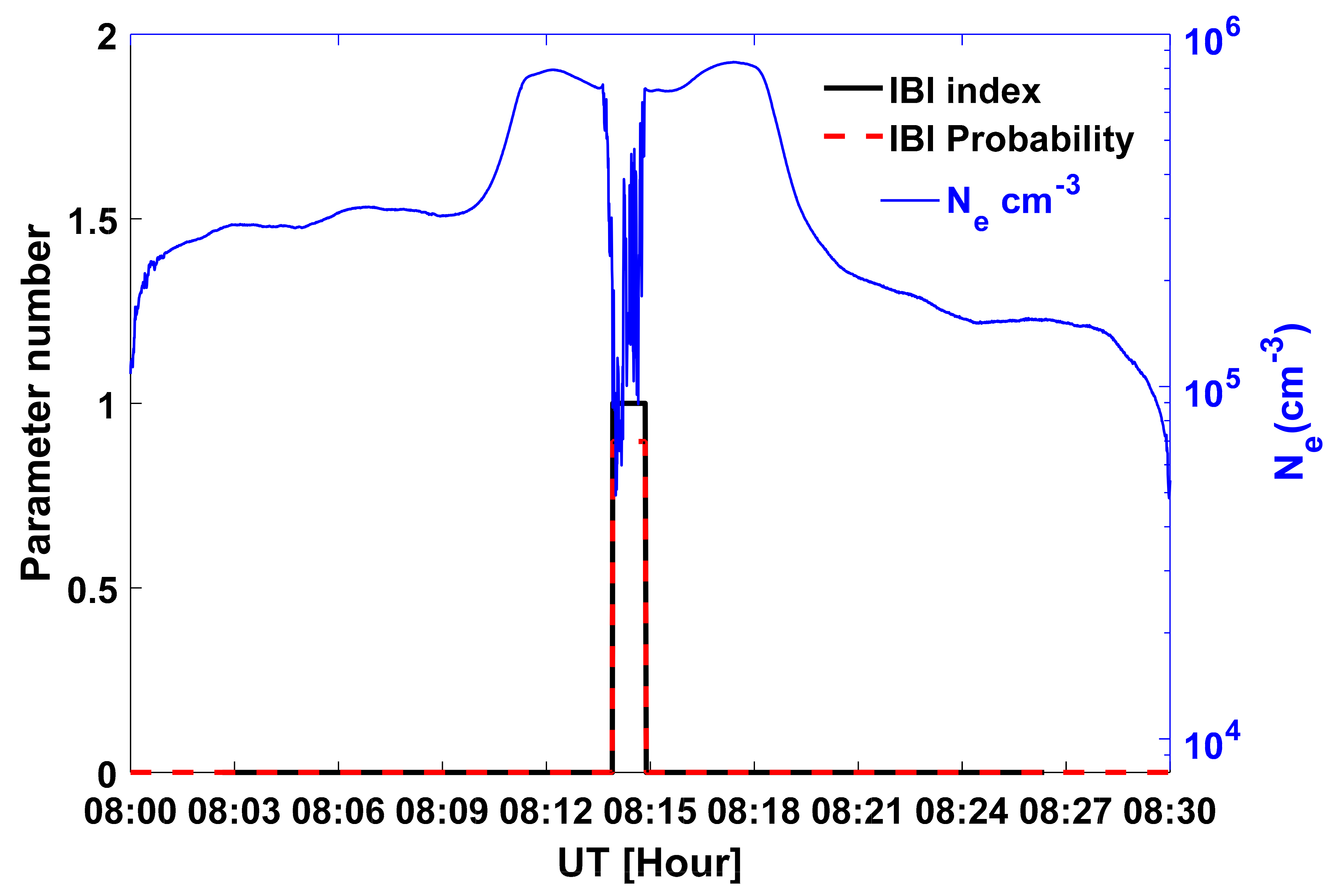
2.2. IBI Selection Criterion

The bubble index indicates every data point as to whether a plasma irregularity is detected.

Table 1. The Bubble index criterion.

Bubble Index	Description
0	Quiet
1	Bubble
−1	Unanalyzable

presents the three potential cases of the bubble index [7]. Bubble index 0 (Quiet) denotes that no small-scale fluctuation is present around that data point. Bubble index 1 (Bubble) means that the data points are impacted by EPBs. Bubble index -1 means unanalyzable IBI event.

According to the authors of [7], the bubble flag is related to exceeding a certain bubble probability level (e.g., >0.8 as stated in [7]). It supports additional information as to why the data point is given as the Bubble Index. In case the Bubble Index equals 0 (Quiet), the related bubble flag is also 0 (Quiet), while if the bubble index equals 1 (Bubbles exist), the related bubble flag may be either 1 (Confirmed Bubble) or 2 (Unconfirmed Bubble) [7]. In our analysis, a bubble flag of 1 (Confirmed Bubble) is chosen, which means the plasma bubble event manifests a high correlation between filtered residual magnetic field strength and filtered plasma density data. Bubble Probability can be defined as the square of the correlation coefficient (known as the coefficient of determination) because EPBs are associated with local enhancement in the magnetic field. If the bubble surpasses a specific threshold probability (e.g., ≥0.5) its bubble flag equals 1, while bubble probability is set to 0 if the bubble index is not equal to 1 or no plasma density data exist around the magnetically detected events (Unconfirmed Bubble). This is because users may set an accurate standard on the relationship between filtered residual strength and filtered plasma density by merging the bubble probability and the bubble index. For our selection of IBI events, we chose events with bubble index equal to 1, bubble flag equal to 1, and bubble probability ≥0.5 and subsequently checked their corresponding $n_e$ irregularities.

Figure 1 is a typical example of a Swarm L2-IBI event. The IBI index and the IBI probability are plotted in solid black and dashed red lines, respectively. The blue line represents the $n_e$ profile along the path of the Swarm B satellite. The event has an IBI index equal to 1 and IBI probability closer to 0.91 as shown in Figure 1, in addition to a bubble flag equal to 1 not shown in Figure 1. These three conditions confirm the existence of a plasma bubble event. We can recognize intense irregularities in the $n_e$ profile between (08:12–08:15 UT) during the same time of the occurrence of the plasma bubble event.

In the present study, we examined seven years of Swarm L2-IBI observations (2014–2020) during geomagnetic storms. We have divided the geomagnetic storms according to [57] into three categories. Moderate storm (−50 nT > Dst > −100 nT), intense storm (−100 nT > Dst > −200 nT), and super storm (−200 nT > Dst > −350 nT).

Table 2. Geomagnetic storms recorded during 2014–2020. Columns from left to right are year, month, day, duration of geomagnetic storm, type of storm, Dst index the number of IBIs occurring from the beginning of the storm until the end of the recovery phase, and finally, the geomagnetic storm driver.

Start Date			Duration	Storm	Dst	Number of IBIs	Storm Driver
Year	Month	Day	(Days)	Type	(nT)
2015	3	17	9	Super	−223	64	CME
2015	6	21	11	Super	−204	33	CME
2014	2	18	5	Intense	−119	1	Weak CME
2015	12	19	5	Intense	−155	15	CME
2015	12	31	5	Intense	−108	0	CME
2016	10	12	8	Intense	−104	19	CME
2017	5	27	4	Intense	−125	1	CME
2017	9	7	5	Intense	−142	10	CME
2018	8	25	6	Intense	−174	0	CME
2014	2	23	4	Moderate	−55	0	CME
2014	2	26	4	Moderate	−97	2	CME
2014	4	29	6	Moderate	−67	4	Solar flare
2014	8	26	10	Moderate	−79	8	CME
2014	10	8	5	Moderate	−51	101	Negative IMF Bz
2014	11	9	19	Moderate	−65	83	CME
2014	12	23	2	Moderate	−57	0	CME
2014	4	11	5	Moderate	−87	5	Negative IMF Bz
2014	9	12	6	Moderate	−88	23	Double CME
2015	2	16	7	Moderate	−64	107	Solar wind streamwind
2015	4	15	6	Moderate	−79	0	CME
2015	7	10	6	Moderate	−61	26	Solar wind stream
2015	7	22	8	Moderate	−63	4	CME
2015	8	22	9	Moderate	−92	5	Solar wind stream of solar wind
2015	9	20	6	Moderate	−75	1	CME
2015	9	7	14	Moderate	−98	1	CME
2015	11	2	5	Moderate	−60	26	Solar wind stream
2015	11	6	10	Moderate	−89	92	CME
2015	1	7	9	Moderate	−99	7	Negative IMF Bz
2015	4	9	5	Moderate	−75	7	CME
2015	6	7	6	Moderate	−73	6	CIR
2015	7	4	7	Moderate	−67	20	CME
2015	8	15	7	Moderate	−84	7	CME
2016	2	2	3	Moderate	−53	1	CIR
2016	2	15	8	Moderate	−57	3	CME
2016	3	14	8	Moderate	−56	24	CME
2016	4	2	6	Moderate	−59	30	CIR
2016	4	12	4	Moderate	−59	19	CME
2016	4	15	3	Moderate	−55	8	CME
2016	8	2	7	Moderate	−52	0	CME
2016	8	23	5	Moderate	−74	3	Solar wind stream
2016	11	9	7	Moderate	−59	0	CME
2016	1	19	7	Moderate	−93	8	CME
2016	5	7	8	Moderate	−88	3	CME
2016	3	5	7	Moderate	−98	11	CIR
2017	3	26	11	Moderate	−74	2	Coronal hole
2017	9	27	8	Moderate	−76	39	CME
2017	11	7	9	Moderate	−94	0	CME
2017	7	16	5	Moderate	−72	0	CME
2018	5	5	9	Moderate	−56	1	Solar wind stream
2018	9	10	7	Moderate	−60	0	CME
2018	11	4	11	Moderate	−53	1	CME
2018	4	19	8	Moderate	−66	0	CME
2018	10	7	7	Moderate	−53	0	CME
2019	8	4	8	Moderate	−50	0	CME
2019	5	10	4	Moderate	−51	0	CME
2019	5	13	3	Moderate	−65	0	CME
2020	2	17	10	Moderate	−52	0	Negative IMF Bz
2020	4	20	2	Moderate	−59	0	CME
2020	7	23	5	Moderate	−52	0	CME

introduces the geomagnetic storms along with their corresponding Dst index values. The hourly Dst index values are obtained from OMNI data (https://omniweb.gsfc.nasa.gov/form/dx1.html (10 January 2020)). The driver of the geomagnetic storm is obtained from the space weather website (https://spaceweather.com/archive.php (20 February 2021)). The driver of the storm could be a Coronal Mass Ejection (CME), a Co-rotating Interaction Region (CIR), a stream of solar wind, or the Interplanetary Magnetic Field turning southward (- IMF Bz). According to Table 2, we have two super storms, seven intense storms, and fifty moderate storms. The total number of IBI events is 831 divided into 97/super storm, 36/intense storm, and 698/moderate storm. According to Table 2, both the two super storms observed in the current study demonstrate a large number of IBIs (97 events). Also, some of the moderate storms showed a larger occurrence rate of IBIs than during super storms.

2.3. COSMIC Mission

COSMIC is a constellation of Low Earth Orbit satellites that probe the Earth’s ionosphere and atmosphere using the mechanism of trans−ionospheric radio wave propagation. The constellation consists of six satellites circled in six circular orbits inclined at ~72° and about 800 km altitude. The satellites provide different kinds of measurements, inclusive GPS-based Radio Occultation (RO) measurements for probing the Earth’s ionosphere and atmosphere. In our study, we investigated the storm-induced variations in the profile shape and the altitude distribution of ionospheric irregularities at different levels of magnetic activities. For this purpose, we used the main COSMIC−RO ionospheric product “ionPrf” ionospheric electron density profiles. We selected IBI events where COSMIC satellites are within $\pm {30}^{°}$ longitudes of the same event observed by the Swarm satellites. The reason for that is to investigate the altitude of the F2 layer peak height (hmF2) and the degree of depletion using COSMIC data for the same IBI event confirmed by the Swarm satellite.

3. Results

In this section, we introduce observational data obtained from Swarm L2−IBI and COSMIC satellites. Our essential aim is to study the morphology and occurrence of the plasma bubbles during three different levels of geomagnetic storms. First, we present a statistical IBI data obtained from the three Swarm satellites to study the variations of plasma bubbles with respect to latitude, longitude, altitude, and local time. Second, we investigate the variation of the ionospheric $n_e$ profile of three geomagnetic storm levels using Swarm and COSMIC satellites.

3.1. The Occurrence Rate of IBIs during Different Types of Geomagnetic Storms

Figure 2 presents a global distribution of IBI events observed by Swarm satellites, occurring during different types of geomagnetic storms with respect to the criteria set in Section 2. IBIs observed during super, intense, and moderate geomagnetic storms are shown in the top, middle, and lower panels, respectively. Events observed by Swarm A, B, and C satellites are marked in red, blue, and cyan dots, respectively. The dashed line marked in magenta color on the world map indicates the ±20° latitude from the dip equator, which is marked in the solid magenta line.

We noticed that regardless of the few IBIs spread farther from the ±20° latitudinal limits, the majority of IBIs were observed closer to or centered around the dip equator. Also, during moderate storms, no IBIs were observed poleward from the ±20° latitudinal limits. In addition, the IBIs observed during moderate and super storms spread over a large range of longitude in comparison with the majority of IBIs during intense storms, which were concentrated within limited longitudes (20° W–90° W). The right column of Figure 2 shows the number of IBIs in the northern and southern hemispheres in magenta and black bars respectively. The range of the Y–axis in both super and intense storms is 15, while for the moderate storm it is expanded to 150 because of the large number of IBIs during moderate storms. We noticed that, 64% of intense storms have a large number of IBI events in the southern hemisphere (Figure 2). In contrast, 59% of moderate and super storms have large IBI events in the northern hemisphere. The number of IBIs in the northern hemisphere is slightly larger than that in the southern hemisphere, at all longitudes, during super, intense, and moderate geomagnetic storms. Consequently, the dramatic increase in the number of IBIs during intense storms within 45° W longitude in the southern hemisphere could be due to the fewer number (36) of IBI events that may mislead the statistical trend.

Swarm B orbits the Earth at higher altitudes (~520) km than Swarm A and C, which orbit the Earth at an average altitude of ~420 km; therefore, the probability of observing IBIs during different types of storms at different altitudes is worth investigation. Figure 3a–c displays the number of IBI events observed by the three Swarm satellites with respect to the geographic longitude during distinct types of storms. The red, blue, and cyan bars correspond to IBIs observed by Swarm A, B, and C satellites, respectively. This shows that during super and intense storms, the number of IBIs at the altitudes of Swarm B (>500 km) is larger than those observed at the altitudes of Swarm A and C. Swarm B recorded about 60% of all the events during super and intense storms and 16% during moderate storms. In contrast, during moderate geomagnetic storms, the number of IBI events observed by Swarm A and C is always larger than those detected by Swarm B as shown in Figure 3c. The occurrence rates of IBIs at the altitudes of Swarm A and C satellites are the maximum (83%) during moderate storms. For all types of storms, the majority of IBI events are observed within the longitudinal sector (0° E and 110° W) or within the location of the SAA.

Figure 4a,b introduces the geographic locations of IBIs observed at different heights according to different storm types. Super, intense, and moderate storms are marked in red, black, and blue dots respectively. These IBIs are superimposed on a map of the total Earth’s main magnetic field that was calculated from the CHAOS−7.4 model at 450 km altitude [58]. The total Earth magnetic field varies up to 60,000 nT as indicated by the color bar index at the rightmost of Figure 4b. The map shows that the minimum magnetic field values of the Earth are located over the Atlantic Ocean between Africa and South America (called SAA). A comparison between the geomagnetic map and the number of IBIs shows that the number of IBIs increases dramatically over SAA at both altitudes.

Figure 4c,d illustrates the number of events at each altitude with respect to longitudes. It clearly shows that at higher altitudes (>500), the majority of events are located within ±20° magnetic latitudes and grouped at longitudes between 10° E and 80° W. In contrast, at lower heights (<470 km), events are spread over larger latitudes (30° N–40° S) and longitudes (30° E–120° W). A comparison between Figure 4c,d shows that the number of IBI events at low altitudes (<470 km) is larger than those observed at higher altitudes (>500 km). Moreover, intense IBIs at high altitudes are only located in a very limited latitude (±10°) and longitudes 20° W to 60° W. At low altitudes, the minimum number of IBIs are associated with intense storms and are scattered over a broad range of latitudes and longitudes, while the maximum number of IBIs are observed during moderate storms. Also, Figure 4c, d shows that the maximum number of IBIs are observed at longitudes 20° E to 120° W. Figure 4c shows that at high altitudes, the numbers of IBIs are comparable during the three types of storms. Comparing the number of IBIs during super storms in Figure 4c,d at both altitudes shows that their corresponding IBI numbers at high altitudes are larger than those at low altitudes. It means the probability of finding IBIs at high altitudes increases with the increase in the level of geomagnetic activity as shown in Figure 4c. Also, the probability of observing IBIs at higher altitudes decreases with the decrease in the geomagnetic activity level as shown in Figure 4d.

3.2. The Local Time Variations of the Occurrence and the Duration Time of IBIs Observed during Different Types of Geomagnetic Storms

The occurrence of IBIs with respect to local time during various types of storms is presented in Figure 5a–c. It is generally noticed that the majority of IBIs are observed between sunset and midnight (18:00–24:00 LT) and few events are observed from post-midnight until the early morning (24:00–06:00 LT). During both super and intense storms, Swarm B recorded a larger number of IBIs in comparison with Swarm A/C. These Swarm B events are observed around the post-sunset hours (18:00–21:00 LT). In contrast during moderate storms, the large number of IBIs are recorded by Swarm A/C and are observed within the pre-midnight hours (21:00–24:00) LT.

At the altitudes of Swarm B, the post-sunset (18:00–21:00 LT) events are larger than those observed within the pre-midnight period. At the altitudes of Swarm A/C, the probability of observing IBIs increases when approaching the pre-midnight hours. Also, the occurrence of the early morning (03:00–06:00 LT) IBIs is larger at the orbits of Swarm A/C.

The duration times of IBIs during super, intense, and moderate geomagnetic storms in red circles, black squares, and blue dots, respectively, are shown in Figure 6a. The occurrence rates of IBIs with duration times <100 s are 65%, 80%, and 73% corresponding to super, intense, and moderate storms, respectively; while for duration times >100 s corresponding to the same order of storms, the occurrence rates are 34%, 19%, and 25%. However, the percentage of IBIs with duration times >100 s is the largest during super storms. Moderate storms showed a larger percentage than intense storms.

Figure 6b shows the duration time of IBIs with respect to the local time at the location orbits of Swarm A, C, and B in red, cyan, and blue dots, respectively. However, both Figure 6a,b show an enhancement in the duration time of IBIs from sunset until midnight. There is no correlation between the duration time of IBIs and the type of the geomagnetic storm as shown in Figure 6a. Also, no correlation was found between the duration time of IBIs and the altitude (the orbit of the satellite) as shown in Figure 6b, as the duration time shows a random distribution with respect to the LT for the three satellites.

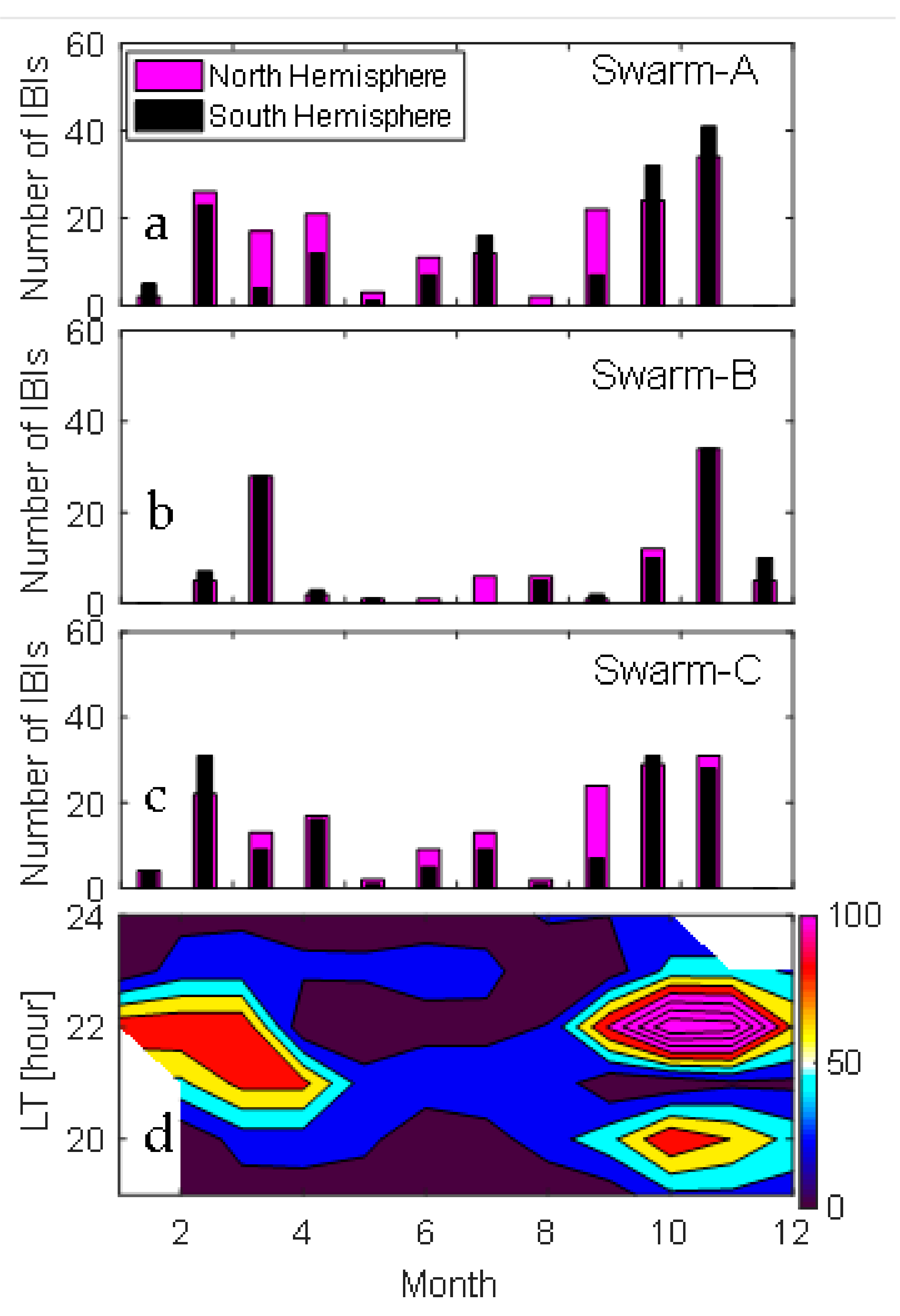
3.3. Seasonal Variations of IBIs at the Altitudes of Swarm Satellites in Both Hemispheres

Figure 7a–c illustrate the number of IBIs with respect to months at the altitudes of Swarm A, B, and C from top to bottom. The numbers of IBIs in the northern and southern hemispheres are marked in magenta and black bars respectively. In both hemispheres, the numbers of IBIs in the months around equinoxes are always larger than the number of IBIs in the summer and winter months. This seasonal variation of the occurrence rate of IBIs is independent of the altitude of Swarm satellites. It is worth noting that we could not make a seasonal variation of the number of IBIs for each type of geomagnetic storm because of the limited number of super and intense storms. This limited number of storms confined the appearance of IBIs within two months during super storms and five months during intense storms as indicated in Table 2. Thereby, the seasonal variations of IBIs during different types of geomagnetic storms are suggested to be investigated in further studies. The number of IBIs in the northern hemispheric summer is larger than in the southern hemisphere. This large occurrence could be attributed to the large electron that develops steeper ${\nabla }_n$ according to Equation (1).

Figure 7d is a contour map of the local time with respect to months for the number of IBIs observed during all types of storms. It shows two maxima of the numbers of IBIs within months 9–11. The first maximum is located within 20:00 LT and the other within 22:00 LT and the minimum number of IBIs is within 21:00 LT. In contrast, months 1–4 have an enhancement in the number of IBIs within 21:00 LT. In the June solstice, there are two small peaks of IBI occurrence, the first around 21:00 LT and the other around 23:00 LT.

Figure 8 shows the seasonal variations of IBIs observed during sunset (17:00–21:00) and pre-midnight (21:00–24:00) local times. IBIs observed by Swarm A, B, and C are marked in red, blue, and cyan colors, respectively. The size of the circle from small to large corresponds to the storm level from moderate to super. The most remarkable points here are, first, the majority of IBIs are observed within the pre-midnight period in all seasons, second, the absence of IBIs during winter months during sunset (local times). The absence of super storm IBIs during the winter months is attributed to the only two super storms that occurred during March and June months. The occurrence of super storm IBIs increases within the pre-midnight period during summer months and sunset during equinoxes. The low occurrence of super EPBs in comparison with moderate EPBs during summer months within the sunset is in agreement with the authors of [53] who found that the number of post-sunset EPBs during quiet periods is larger than those observed during disturbed periods. This low occurrence of super storm IBIs during summer months (sunset) is reversed in local time during equinoxes, which is a novel feature of IBIs in our analysis. The absence of sunset IBIs during winter months could be attributed to the trans−equatorial wind that suppresses the occurrence of EPBs in the winter hemisphere as reported in previous studies, but confirming this suggestion needs further investigation.

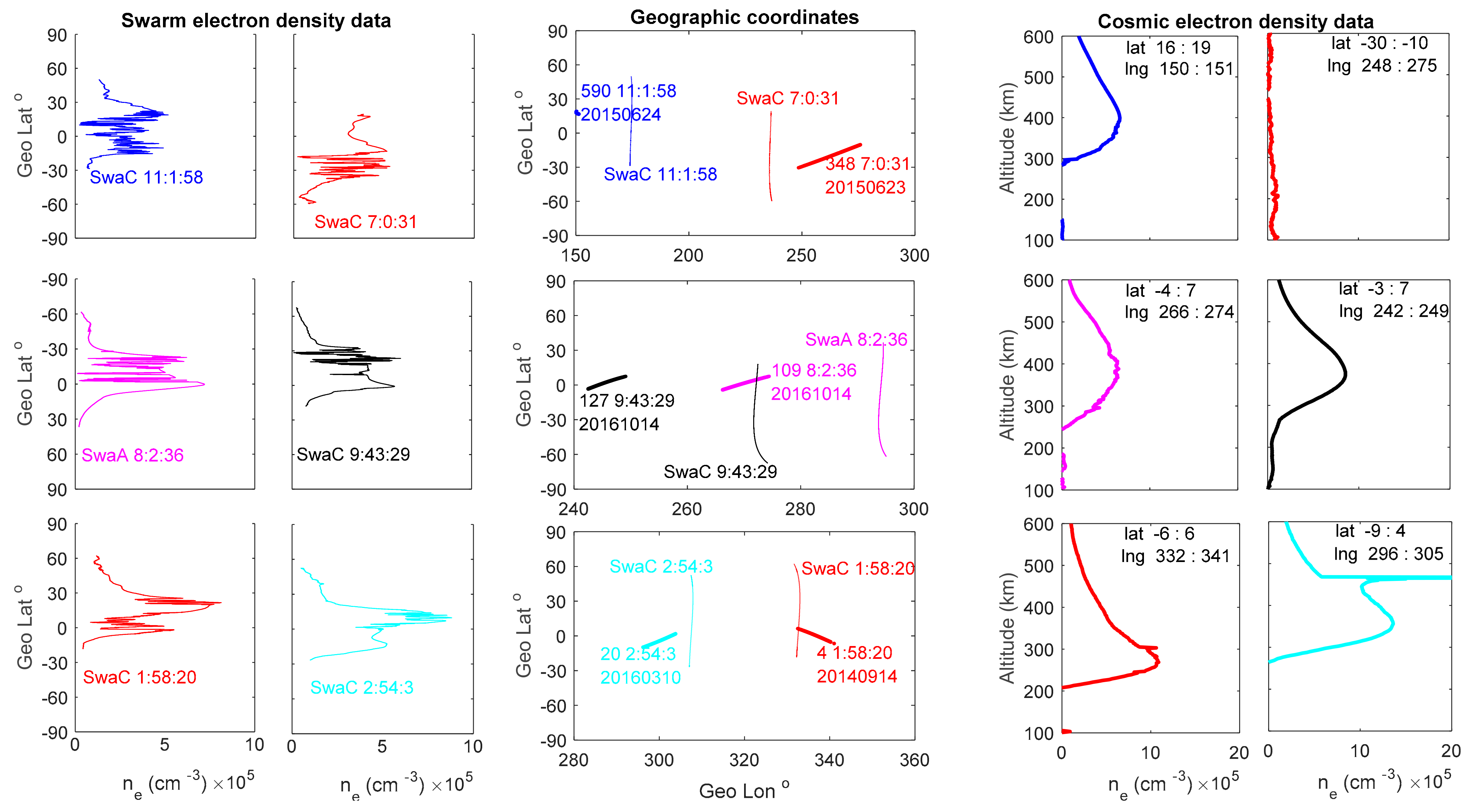
3.4. A Qualitative Investigation of IBI Events Using Swarm and COSMIC $n_e$ Data

To conduct a qualitative investigation of the response of the topside ionospheric $n_e$ profile under different levels of geomagnetic activities, we compared plasma density measurements from Swarm satellites and COSMIC $n_e$ profiles. Figure 9 shows the latitudinal and altitudinal profiles of the $n_e$ observed by Swarm and COSMIC satellites in the left and right columns, respectively. The middle column of Figure 9 illustrates the location of Swarm and COSMIC satellites. Rows ordered from top to bottom corresponding to IBIs during super, intense, and moderate storms, respectively. The same event observed by both Swarm and COSMIC satellites is marked in the same color. The occurrence time of each IBI event is indicated in the middle column of Figure 9. For each type of storm, we found only two IBI events for each type of storm where COSMIC locates within $\pm {30}^{°}$ longitude from Swarm.

During super storms (upper row), the $n_e$ data are not only dramatically decreased/depleted in comparison with other storms, but also the hmF2 is displaced to higher altitudes ~ 400 km. However, these two features are not observed simultaneously for the same event, they are clearly observed independently in our observations of the IBIs occurring on 23 and 24 June 2015. COSMIC−RO observation extends to broad longitudes as shown in the middle panel of the upper row, which means irregularities observed by Swarm satellites extend to large longitudes. Also, Swarm $n_e$ data are intensively disturbed/depleted over a wide range of latitudes due to the existence of large plasma irregularities, which could be seen along the path of Swarm satellites. Moderate geomagnetic storms show low $n_e$ degradation in comparison with super and intense geomagnetic storms. Also, the hmF2 is observed at lower altitudes. Several authors have attributed the intense dynamics of the ionospheric irregularities during super geomagnetic storms to auroral activities [59]. Regardless, the degradation degree increases with the storm activity level, it is hard to correlate it with the size of areas exposed to degradation. This issue is difficult to investigate using the $\pm {30}^{°}$ longitude criterion because of the fewer number of space observatories whereas COSMIC is closer to Swarm for the same IBI event.

Geomagnetic storms observed on June 2015, October 2016, and September 2014 corresponding to super, intense, and moderate types were analyzed in detail using the COSMIC $n_e$ data shown in the left, middle, and right columns, respectively, in Figure 10. Rows from top to bottom correspond to the SYMH index, the hmF2, and the $n_e$ at the hmF2, respectively. The SYMH index shows a strong depression in the Earth’s magnetic field (<−250 nT) on June 23, 2015, corresponding to the super storm criterion set in the data and methodology sections, but on September 14, 2014, there was a low depression in the Earth’s magnetic field corresponding to a moderate storm. The number of IBIs on each day of the storm is superimposed in the form of bars in the same panel of the SYMH index. The number of IBIs during the main phase of the super and intense storms is clearly larger than those that occurred during the recovery phase. This enhanced number of IBIs during the main phase is in agreement with previous studies that correlate the occurrence rate of IBIs with the activity level and the main phase of geomagnetic storms [60,61,62,63]. The reason for that is the PPEF, which is transmitted instantaneously into the equatorial region during the convection processes and becomes intensified during the main phase. Therefore, if we expect the PPEF to be the main driver of IBIs observed during the main phases of intense and super storms, another question arises regarding the IBIs observed during the recovery phase of all storms. This indicates the insignificant role of the PPEF in the generation mechanism of the IBIs. Therefore, another mechanism such as the DDEF or the shielding electric field could be the main reason for generating IBIs during the recovery phase of the storms.

The geographic coordinates and the altitudes of the noontime hmF2 were recorded for each COSMIC profile. The selected noontime events vary from 12:00 LT to 16:00 LT. Subsequently, the selected data were binned into 10 degrees in latitude and one hour UT, where the median altitudinal and $n_e$ values within this binned area were calculated as shown in the middle and lower rows of Figure 10, respectively. Results indicate that, the ionospheric hmF2 varies with respect to the type of geomagnetic storm. The hmF2 was observed to be strongly raised to high altitudes only within the main phase of the super storm, but through the whole recovery phase, it was observed at lower altitudes, while during the moderate storm it was always observed at higher altitudes. The hmF2 of super and intense storms was similar, which was always observed at lower altitudes in comparison with moderate storms. Also, the hmF2 was larger in the northern hemisphere during super storm and strongly shifted poleward from the equator. The large altitudes of the northern hemispheric hmF2 during super storms could be attributed to the trans−equatorial wind, which flows from the summer (northern) hemisphere to the winter (southern) hemisphere and subsequently raises the hmF2 to large altitudes in the summer/northern hemisphere. During intense and moderate geomagnetic storms, the hmF2 is centered on the equator. The reason for this is that, both storms are observed within the autumn equinox.

The $n_e$ profile corresponding to the three types of storms in the lower row shows strong depletion of $n_e$ during super storms in comparison with moderate storms, while in intense storms, it exhibits an intermediate state. Also, the double crests due to the equatorial ionization anomaly in both hemispheres appeared clearly during the moderate geomagnetic storm (panel in the rightmost bottom) and disappeared during super storms (panel in the leftmost bottom).

4. Discussion

As shown in the previous section, we have introduced our observations of the morphology of EPB events recorded by Swarm satellites during different types of geomagnetic storms recorded from 2014 to 2020. We have investigated 59 geomagnetic storms (2 super, 7 intense, and 50 moderate storms) under our classification set in Section 2. A list of 831 IBI events was recorded by the Swarm constellation during all storms.

Figure 2, shows that most IBIs are located within ±20° geomagnetic latitudes and between 90° W and 20° E corresponding to the location of the SAA. The plasma drift velocity $v_z$ is related to the Earth’s magnetic and electric fields in the following form ($v_z\mathit{\propto } \frac{E}{B})$. Therefore, within the dusk sector, the eastward electric field is greatest and subsequently, the R − T irregularities increase rapidly. The number of IBIs in the northern hemisphere is always larger than those in the southern hemisphere. The north−south hemispheric asymmetry of the IBIs in summer months could be attributed to the large electron density which develops steeper ${\nabla }_n$ according to Equation (1) [17,46]. Also, it is worth noting that the large electron density during equinoxes [55] is considered the main reason behind the large equinoctial IBIs. Also, the authors of [53] proposed that the increase in the background plasma density at the topside F region improves the EPB development in two ways: by enhancing the growth of EPD along the flux tube or by maintaining EPB rising upward.

According to individual storms listed in Table 2, the occurrence rate of IBIs is not necessarily increasing with the storm level, as several moderate geomagnetic storms recorded a large number of IBIs in comparison with super storms. These results are in agreement with the authors of [62] who found that the occurrence of EPBs is suppressed or enhanced for individual storm cases.

Generally, we have found a large occurrence of IBIs after sunset times. One of the most significant creation techniques of plasma irregularities within this time is the prereversal enhancement (PRE) eastward electric field [64]. The PRE can supply a suitable circumstance for evolving the R–T instability and raising the equatorial upward drift velocity. The probability of observing EPB at high altitudes (the orbit of Swarm B) increases with the increase in the geomagnetic storm level as shown in Figure 3 and Figure 5. The altitudinal analysis of EPBs presented by the authors of [65] found that the post-midnight EPBs extend to higher altitudes over the African and American sectors. According to Figure 4, these regions are characterized by low magnetic field strength; therefore, the growth rate of EPBs according to Equation (1) is very large. Our analysis shows that, not only does the occurrence rate of IBIs increase over the African and American regions but also, the probability of observing IBIs at high altitudes (orbit of Swarm B) increases during super storms, as shown in Figure 5a. Regardless, the author of [66] found a significant reduction in the height of the F layer within the evening hours and significant enhancement in the post-midnight period of the April 24, 2012 magnetic storm, suppression in the number of IBIs was observed during these local times. They attributed this suppression to the westward electric field associated with the DDEF or other factors such as injection of the ring current and the IMF Bz. Therefore, the large occurrence of IBIs at high altitudes during super storms in our analysis could be interpreted in terms of the enhanced eastward electric field. The enhanced strength of the electric field forces plasma to move into higher altitudes and increases the probability of observing IBIs at higher altitudes especially within the post-sunset period. This suggestion is acceptable only in case of no injection to the ring current and if the IMF Bz is positive. Further studies could distinguish the altitudinal behavior of IBIs with respect to the DDEF, ring current injection, and IMF Bz.

The duration time of IBIs during super, intense, and moderate geomagnetic storms is independent of the type of storm. It also has no correlation with the altitude of the satellite as shown in Figure 6a,b. The duration time of IBIs is only larger from sunset to midnight and independent of the type of the geomagnetic storm and the altitude of the satellite, as it demonstrates a random distribution during different types of geomagnetic storms. It also becomes very large around the SAA region (not shown). According to this observation, if the electric field strength is the main controller in the duration time (Spatial scale) of IBIs, we would find a high correlation between the duration time and the type of the geomagnetic storm level and an inverse relationship between the duration time and the altitude. Because the large electric field strength raises plasma into higher altitudes (orbits of Swarm B) as obtained in Figure 3 and Figure 5, subsequently low altitudinal ionospheric regions would persist degraded from plasma for longer times than those at higher altitudes especially during super storms. Therefore, this result suggests that the electric field strength has an insignificant contribution to the duration time of IBIs. The enhancement of the duration time of IBIs within the dusk side over the SAA region could be interpreted in terms of the high gradient in the electron density and the depression in the Earth’s magnetic field. These are the main factors that could control the scale size (duration time) of the IBI event.

A large occurrence of IBIs is recorded within equinox months (February to April and September to November) is shown in Figure 7, which is consistent with previous studies in [61,65] and references therein. It could be interpreted in terms of the enhanced thermospheric zonal wind during equinoxes [67]. This wind motivates the vertical Pedersen currents that can polarize the initial density disturbance into an unstable mode to trigger plasma bubbles [68].

The low occurrence of IBIs during summer months in both hemispheres is due to the trans−equatorial wind which suppresses the growth rate of the R−T instability [62]. Figure 7a–c confirm that seasonal variations of IBIs during the three types of storms recorded in Table 2 are consistent with the general trend of the seasonal occurrence of IBIs reported in [65]. The trans−equatorial wind may cause a reduction in the local conductivity on the upwind side (summer hemisphere) where the layer is raised and cause an increase in the local conductivity on the downwind side (winter hemisphere) where the layer is lowered. Subsequently, the instabilities in density irregularities near the bubble boundaries may be suppressed in the winter due to the shorted polarization electric field arising from the high conductivity. This might contribute to the slightly lower occurrence rate of the irregularities in the winter hemisphere than the summer hemisphere as shown in Figure 7a–c. The enhanced occurrence of IBIs after sunset times is attributed to the low flux tube integrated conductivity at low magnetic latitudes, where the magnetic field lines are aligned with the terminator [16,69]. The double small peaks of the IBI occurrence during June solstice around 21:00 and 23:00 are similar to those presented in Figure 6b in [65], but the large double peaks within months 9–12 are different from the single equinoxes’ occurrence EPBs peak presented in [65].

The enhancement of super storm IBIs during summer months within the pre-midnight and sunset periods during equinoxes is an interesting observation and needs further investigation. Although the authors of [70] observed an enhancement of the EPBs with the activity level within the post-sunset period (18:00–24:00 LT) during equinoxes, our division of post-sunset LTs into sunset (17:00–21:00 LT) and pre–midnight (21:00–24:00) periods shows deeper details regarding the exact LT enhancement of EPBs with respect to the storm type as shown in Figure 8.

IBI events observed within the 22–25 June 2015 super storm are marked by a vertical red line as shown in Figure 11c. The IBI event on June 23, appeared within the post-midnight (~01:00 LT) period after the occurrence of an intense geomagnetic substorm as shown in Figure 11b. The occurrence of a geomagnetic substorm is clearly indicated by the strong negative variation in the AL index (−1500 nT) at 05:00 UT on June 23. This substorm is also associated with large negative IMF B_z (−40 nT) and positive electric field variation in red solid and black dotted lines, respectively, as shown in Figure 11a, which means a strong injection into the magnetosphere. The depletion of the $n_e$ is associated with the IBI event observed a few hours later at 07:00 UT on the same day. Therefore, the occurrence of IBI could be interpreted in terms of the DDEF which develops a few hours after a geomagnetic substorm. This eastward nightside DDEF has the capability to raise plasma to higher altitudes and subsequently depletes plasma in lower altitudinal ionospheric regions. This is in agreement with the authors of [20] who suggested the DDEF as the main controller of the low latitude ionospheric instabilities which appear a few hours after the start of the storm main phase. In addition, the authors of [63] stated that the DDEF remains for several days during the storm recovery phase, which is clearly inferred from the IBIs occurring during the recovery phase of the moderate geomagnetic storm shown in Figure 10. Also, the authors of [53] stated that after the onset, the DDEF is the main driver of the equatorial plasma depletion because it appeared 5 h after the IMF Bz turned southward during the recovery phase.

Similarly, the IBI event observed on June 24 at 11:00 UT, occurred within the pre-midnight (~22:20 LT) period a few hours after the occurrence of the geomagnetic substorm occurred at 09:30 UT. This IBI event was observed during the insignificant variations in both the IMF B_z and electric field, which means the PPEF has no role in creating such an IBI event. However, both the IMF Bz and the electric field have small negative and positive variations respectively, the hmF2 peak of this event rose to higher altitudes (~400 km), which confirms our suggestion about DDEF.

5. Conclusions

By examining seven years of Swarm L2−IBI data, we studied the occurrence rate of the equatorial plasma bubbles (EPBs) during different levels of geomagnetic storms. The main findings can be summarized in the following:

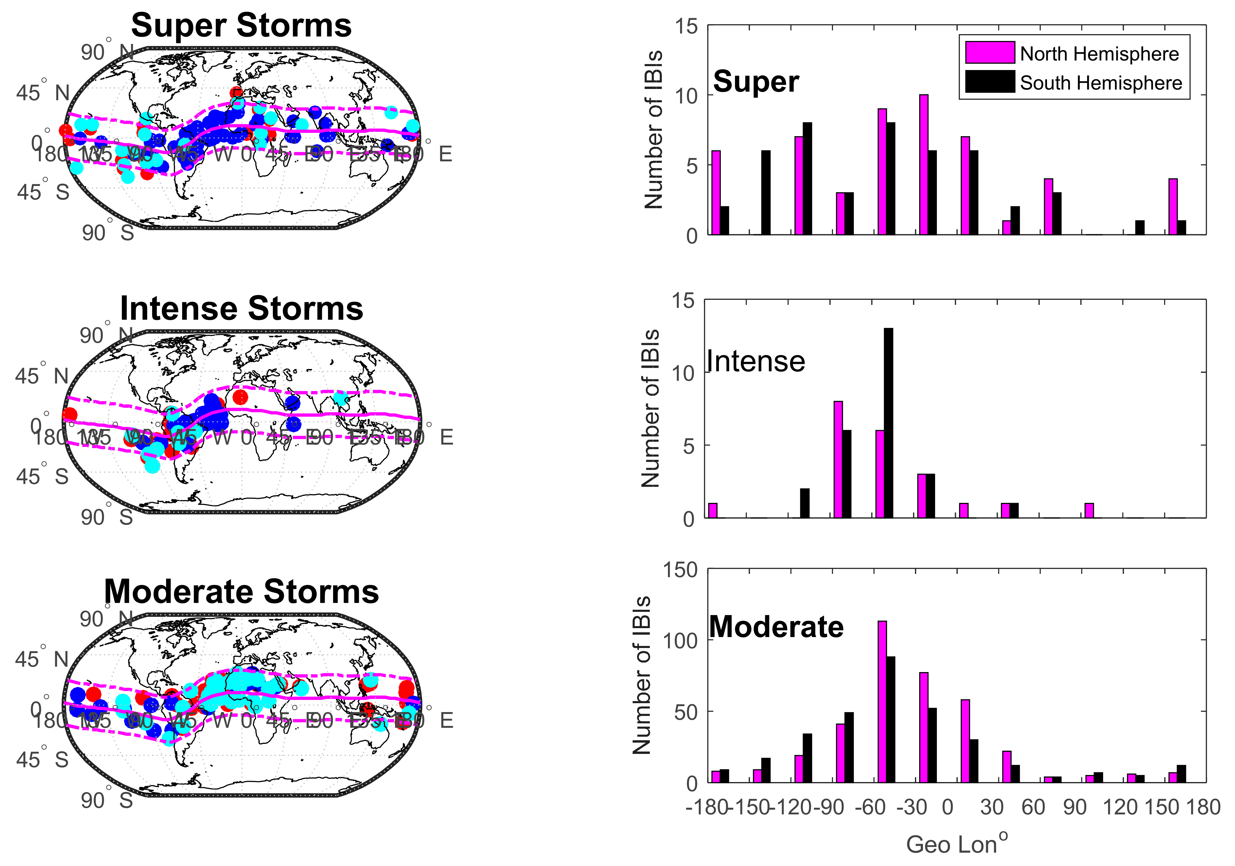
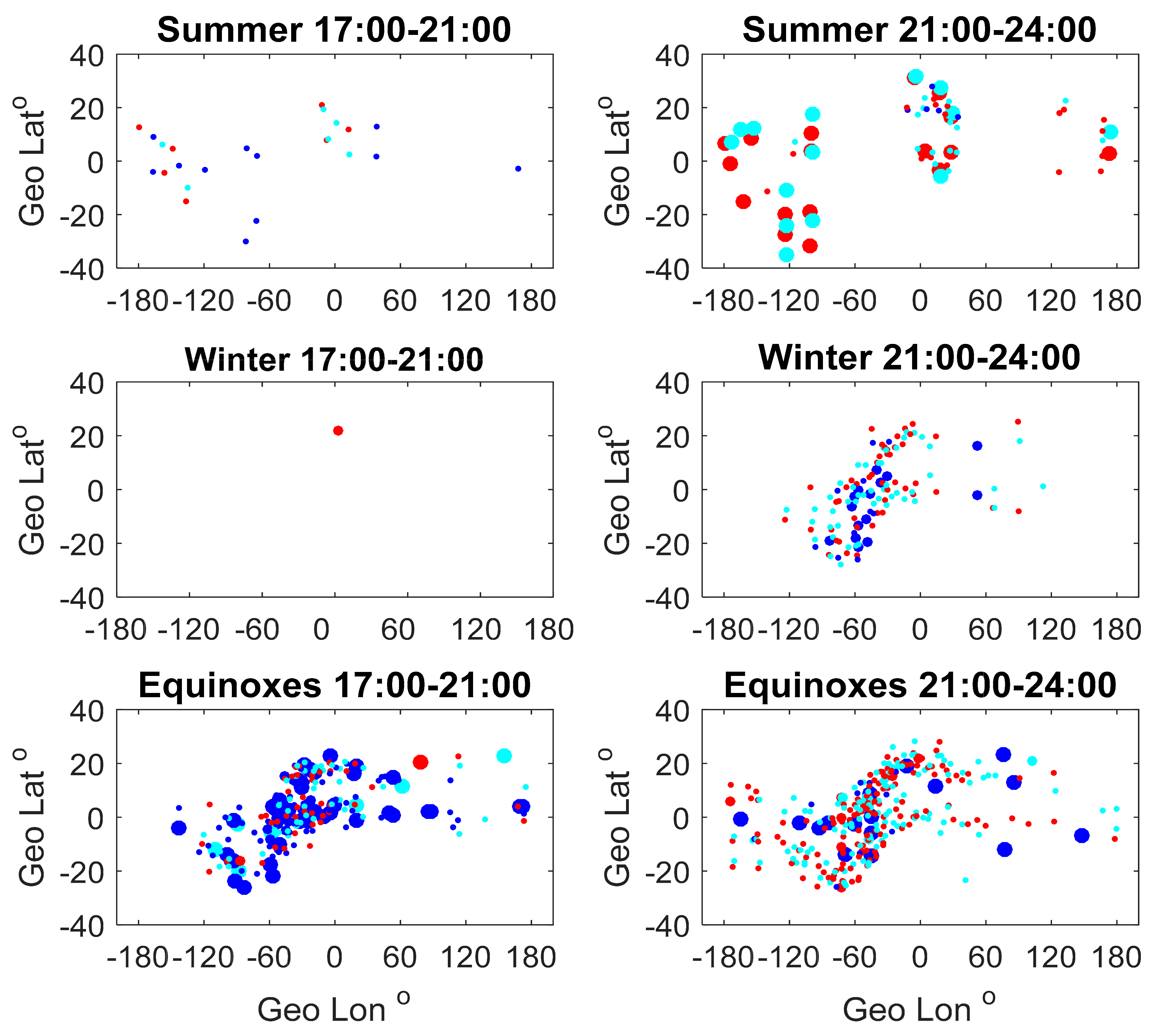
• The majority of IBIs are observed within ±20° latitude around the dip equator. The IBIs observed during moderate and super storms spread over a large range of longitude in comparison with the IBIs observed during intense storms, which are concentrated within limited longitudes over the SAA. The numbers of IBIs in the northern hemisphere are always slightly larger than their corresponding southern hemispheric numbers at all longitudes during super, intense, and moderate geomagnetic storms.
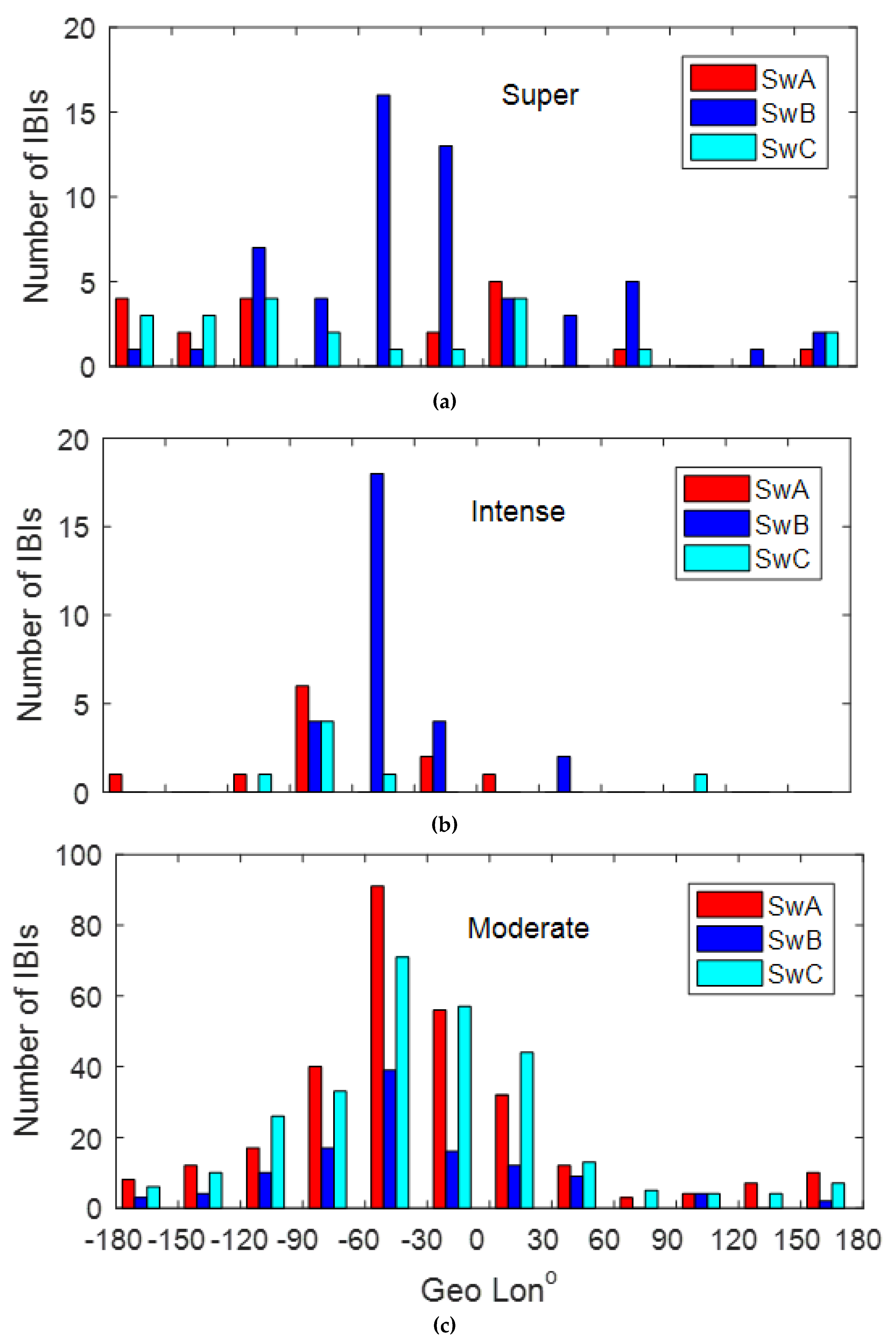
• During super and intense storms, the number of IBIs at the altitudes of Swarm B is larger than those observed at the altitudes of Swarm A and C. During moderate storms the majority number of IBIs are observed by Swarm A and C. Irrespective of storm type, the plasma bubble events have a noticeable longitudinal distribution, as the majority of IBI events are observed within the longitudinal sector (0° E and 110° W), where the SAA is located.
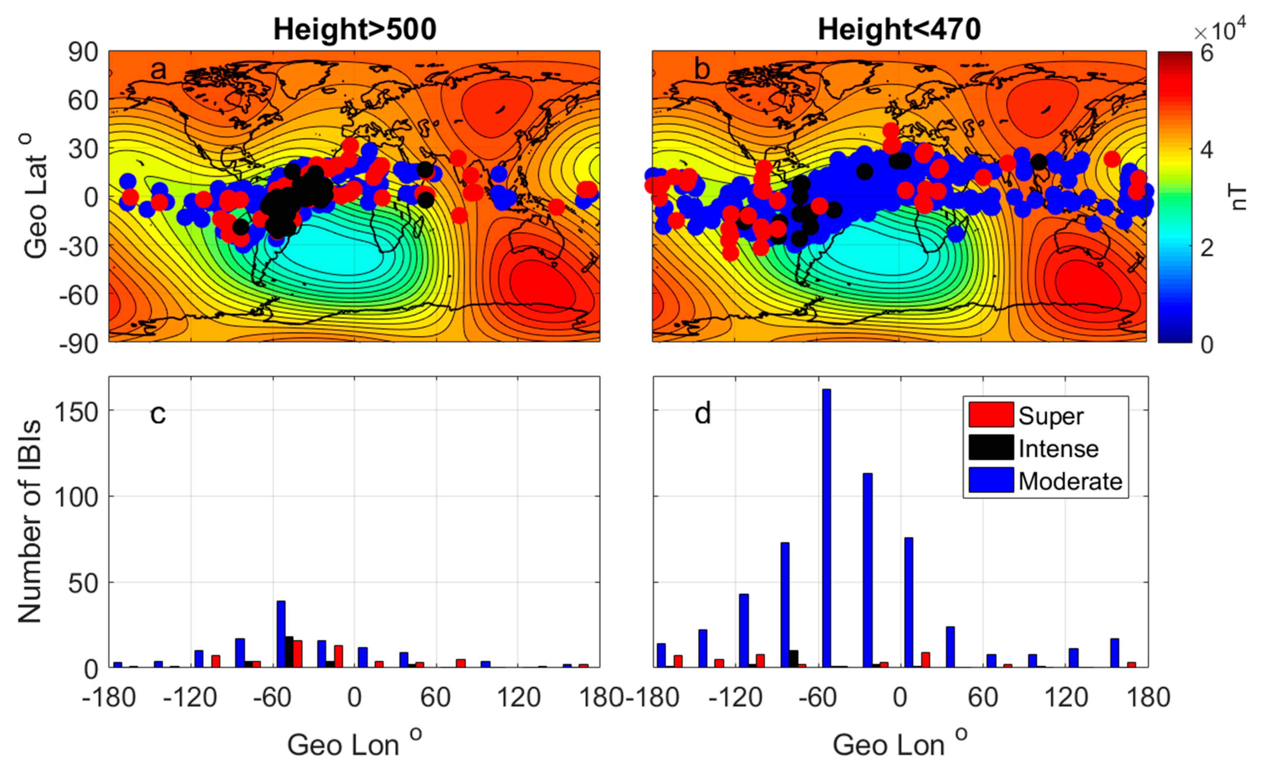
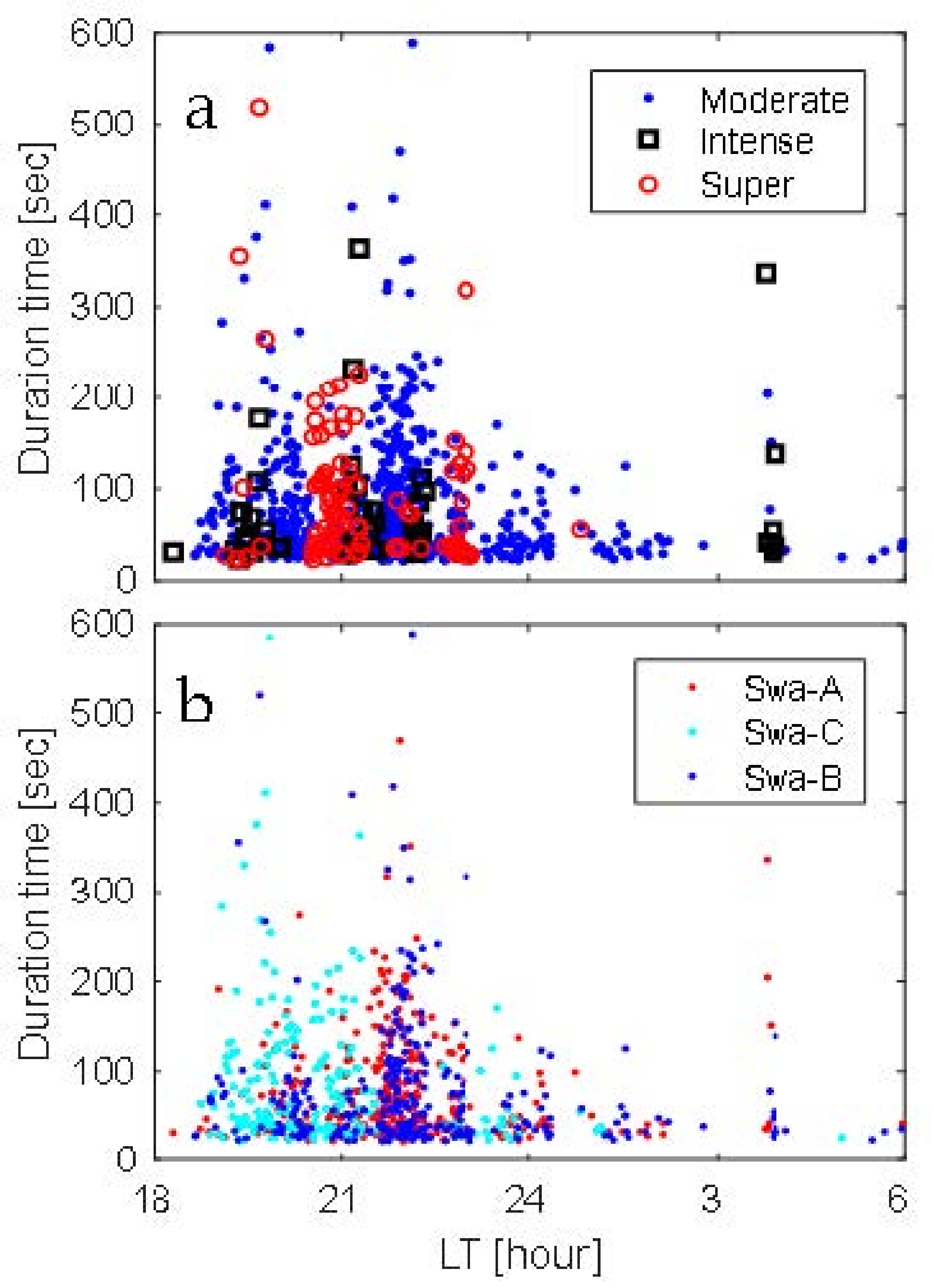
• The number of IBI events at low altitudes (˂470 km) is larger than those observed at higher altitudes (˃500 km) and the probability of finding IBIs at higher altitudes increases with the increase in the level of the geomagnetic storm. No correlation was found between the duration time (scale) of the IBIs and the altitudes because the duration time of IBIs has a random distribution at both altitudes for all types of storms. The duration time only tends to have a significant enhancement over the SAA region.
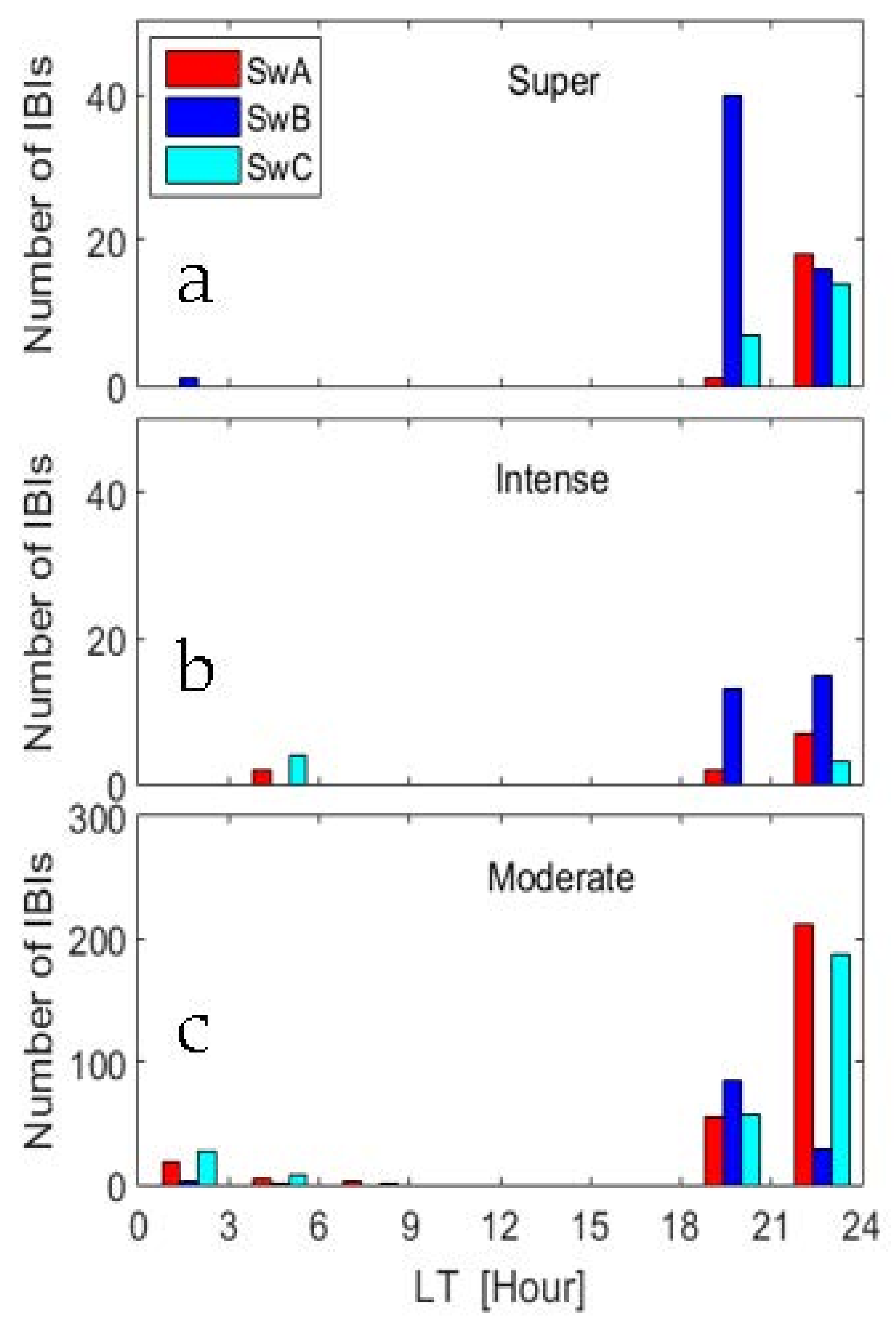
• The local time variation of IBI events shows distinguished patterns over different types of storms. During super storms, the maximum number of IBIs detected by Swarm A and C appeared within the pre-midnight hours (21:00–24:00 LT) and shifted to sunset hours (18:00−21:00 LT) for Swarm B. On the other hand, during intense storms, the probability of observing IBIs by Swarm (A, C) in post-midnight hours (24:00–6:00 LT) is larger in comparison with the super storms. The occurrence rate of IBIs during moderate storms increases with approaching the pre-midnight (21:00–24:00 LT) time. Moreover, the number of IBIs at the altitudes of Swarm A and C is always larger than those observed by Swarm B. In addition, the number of events detected by the three satellites within the post-sunset is larger than those observed within the pre-midnight period.
• The occurrence rate of IBIs with duration times >100s is larger during super storms while the moderate storms showed a larger percentage than intense storms. So, no correlation was found between the duration time of IBIs and the type of geomagnetic storm. The duration time of IBIs only increases from the sunset until midnight, and also over the SAA region. Also, the most remarkable point is the absence of sunset IBI events during the winter months. In addition, the majority of super storm IBIs are only observed within the pre-midnight period during summer months and within the sunset period during equinoxes.
• The seasonal variations of IBIs indicated that the numbers of IBIs in the equinoxes are always larger than those in the summer and winter months. This seasonal variation is independent of the altitude of Swarm satellites. Moreover, the number of IBIs has two crests: one at 20:00 LT and the other at 22:00 LT during months 9–11.
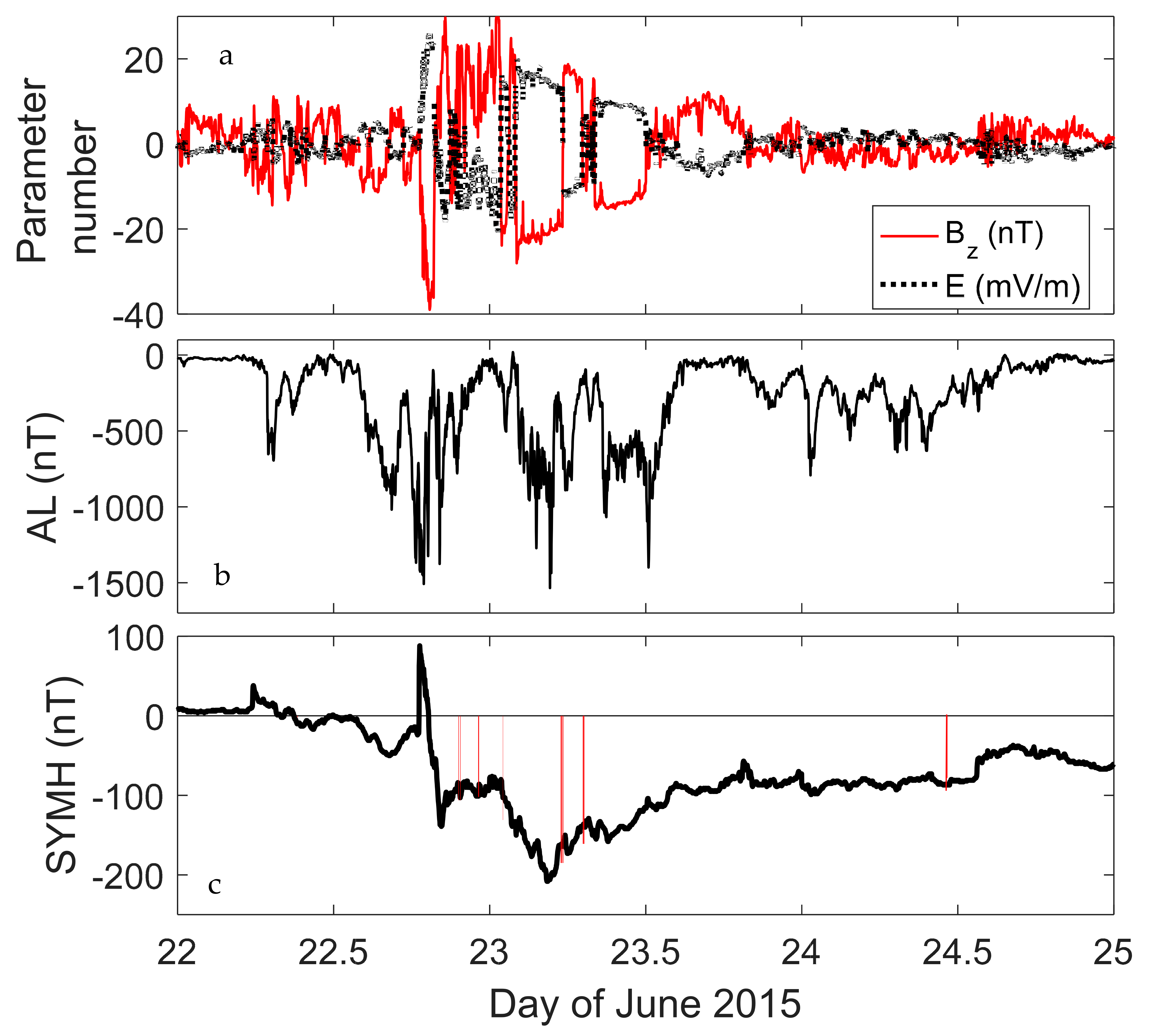
• COSMIC electron density at the F2 layer peak height (hmF2) layer showed that, during super storms, the $n_e$ data are dramatically decreased/depleted in comparison with moderate and intense storms. The hmF2 is displaced to higher altitudes (~400 km) not only during the main phase of super storms but during intense storms and in the recovery phase of super storms, it is observed at lower altitudes in comparison with moderate storms.
• IBIs are found to be observed a few hours later than the onset time of geomagnetic substorms. Therefore, the probable driver of IBIs is suggested to be the DDEF.

References

1. Kelly, M.C.; Heelis, R.A.; Plumb, R.A.; Marshall, J. The Earth’s Ionosphere: Plasma Physics and Electrodynamics; Academic Press: Cambridge, MA, USA, 1989. [Google Scholar]
2. Woodman, R.F.; La Hoz, C. Radar observations of F region equatorial irregularities. J. Geophys. Res. 1976, 83, 5447–5466. [Google Scholar] [CrossRef]
3. Ott, E. Theory of Rayleigh−Taylor bubbles in the equatorial ionosphere. J. Geophys. Res. Space Phys. 1978, 83, 2066–2070. [Google Scholar] [CrossRef]
4. Ossakow, S.L. Spread−F theories—A review. J. Atmos. Terr. Phys. 1981, 43, 437–452. [Google Scholar] [CrossRef]
5. Keskinen, M.J.; Ossakow, S.L.; Basu, S.; Sultan, P.J. Magnetic−flux−tube−integrated evolution of equatorial ionospheric plasma bubbles. J. Geophys. Res. Space Phys. 1998, 103, 3957–3967. [Google Scholar] [CrossRef]
6. Hanson, W.B.; Sanatani, S. Large Ni gradients below the equatorial F peak. J. Geophys. Res. 1973, 78, 1167–1173. [Google Scholar] [CrossRef]
7. Park, J.; Noja, M.; Stolle, C.; Lühr, H. The Ionospheric Bubble Index deduced from magnetic field and plasma observations onboard Swarm. Earth Planets Space 2013, 65, 1333–1344. [Google Scholar] [CrossRef] [Green Version]
8. Aarons, J. The longitudinal morphology of equatorial F−layer irregularities relevant to their occurrence. Space Sci. Rev. 1993, 63, 209–243. [Google Scholar] [CrossRef]
9. Kelley, M.C.; Makela, J.J.; Paxton, L.J.; Kamalabadi, F.; Comberiate, J.M.; Kil, H. The first coordinated ground− and space−based optical observations of equatorial plasma bubbles. Geophys. Res. Lett. 2003, 30. [Google Scholar] [CrossRef]
10. Kil, H.; Su, S.; Paxton, L.J.; Wolven, B.C.; Yeh, H.C.; Zhang, Y.; Morrison, D. Coincident equatorial bubble detection by TIMED/GUVI and ROCSAT−1. Geophys. Res. Lett. 2004, 31. [Google Scholar] [CrossRef]
11. Makela, J.J.; Kelley, M.C. Field−aligned 777.4−nm composite airglow images of equatorial plasma depletions. Geophys. Res. Lett. 2003, 30, 25–31. [Google Scholar] [CrossRef]
12. Burke, W.; Donatelli, D.; Sagalyn, R.; Kelley, M. Low density regions observed at high altitudes and their connection with equatorial spread F. Planet. Space Sci. 1979, 27, 593–601. [Google Scholar] [CrossRef]
13. Huang, C.-S.; Foster, J.C.; Sahai, Y. Significant depletions of the ionospheric plasma density at middle latitudes: A possible signature of equatorial spread F bubbles near the plasmapause. J. Geophys. Res. Space Phys. 2007, 112. [Google Scholar] [CrossRef]
14. Kil, H.; Lee, W.K.; Paxton, L.J.; Hairston, M.R.; Jee, G. Equatorial broad plasma depletions associated with the evening prereversal enhancement and plasma bubbles during the 17 March 2015 storm. J. Geophys. Res. Space Phys. 2016, 121, 10209–10219. [Google Scholar] [CrossRef]
15. Scherliess, L.; Fejer, B.G. Storm time dependence of equatorial disturbance dynamo zonal electric fields. J. Geophys. Res. Space Phys. 1997, 102, 24037–24046. [Google Scholar] [CrossRef]
16. Huang, C.Y.; Burke, W.J.; Machuzak, J.S.; Gentile, L.C.; Sultan, P.J. Equatorial plasma bubbles observed by DMSP satellites during a full solar cycle: Toward a global climatology. J. Geophys. Res. Space Phys. 2002, 107, SIA 7-1–SIA 7-10. [Google Scholar] [CrossRef]
17. Huang, C.Y.; Burke, W.J.; Machuzak, J.S.; Gentile, L.C.; Sultan, P.J. DMSP observations of equatorial plasma bubbles in the topside ionosphere near solar maximum. J. Geophys. Res. Space Phys. 2001, 106, 8131–8142. [Google Scholar] [CrossRef]
18. Ghamry, E.; Lethy, A.; Arafa−Hamed, T.; Elaal, E.A. A comprehensive analysis of the geomagnetic storms occurred during 18 February and 2 March 2014. NRIAG J. Astron. Geophys. 2016, 5, 263–268. [Google Scholar] [CrossRef] [Green Version]
19. Abiriga, F.; Amabayo, E.B.; Jurua, E.; Cilliers, P.J. Statistical characterization of equatorial plasma bubbles over East Africa. J. Atmos. Sol. Terr. Phys. 2020, 200, 105197. [Google Scholar] [CrossRef]
20. Zhou, Y.-L.; Lühr, H.; Xiong, C.; Pfaff, R.F. Ionospheric storm effects and equatorial plasma irregularities during the 17–18 March 2015 event. J. Geophys. Res. Space Phys. 2016, 121, 9146–9163. [Google Scholar] [CrossRef] [Green Version]
21. Hashimoto, K.K.; Kikuchi, T.; Tomizawa, I.; Hosokawa, K.; Chum, J.; Buresova, D.; Nose, M.; Koga, K. Penetration electric fields observed at middle and low latitudes during the 22 June 2015 geomagnetic storm. Earth Planets Space 2020, 72, 1–15. [Google Scholar] [CrossRef]
22. Zhang, K.; Li, X.; Xiong, C.; Meng, X.; Li, X.; Yuan, Y.; Zhang, X. The Influence of Geomagnetic Storm of 7–8 September 2017 on the Swarm Precise Orbit Determination. J. Geophys. Res. Space Phys. 2019, 124, 6971–6984. [Google Scholar] [CrossRef]
23. Nishida, A. Coherence of geomagnetic DP 2 fluctuations with interplanetary magnetic variations. J. Geophys. Res. 1968, 73, 5549–5559. [Google Scholar] [CrossRef] [Green Version]
24. Fejer, B.G.; Jensen, J.W.; Su, S.Y. Seasonal and longitudinal dependence of equatorial disturbance vertical plasma drifts. Geophys. Res. Lett. 2008, 35. [Google Scholar] [CrossRef]
25. Kobea, A.T.; Emery, B.A.; Peymirat, C.; Luhr, H.; Moretto, T.; Hairston, M.; Amory-Mazaudier, C.; Richmond, A.D. Electrodynamic coupling of high and low latitudes: Observations on May 27, 1993. J. Geophys. Res. Space Phys. 2000, 105, 22979–22989. [Google Scholar] [CrossRef] [Green Version]
26. Peymirat, C.; Richmond, A.D.; Kobea, A.T. Electrodynamic coupling of high and low latitudes: Simulations of shielding/overshielding effects. J. Geophys. Res. Space Phys. 2000, 105, 22991–23003. [Google Scholar] [CrossRef]
27. Fejer, B.G.; Emmert, J.T. Low−latitude ionospheric disturbance electric field effects during the recovery phase of the 19–21 October 1998 magnetic storm. J. Geophys. Res. Space Phys. 2003, 108. [Google Scholar] [CrossRef]
28. Ritter, P.; Lühr, H.; Doornbos, E. Substorm−related thermospheric density and wind disturbances derived from CHAMP observations. Ann. Geophys. 2010, 28, 1207–1220. [Google Scholar] [CrossRef] [Green Version]
29. Xiong, C.; Lühr, H.; Fejer, B.G. Global features of the disturbance winds during storm time deduced from CHAMP observations. J. Geophys. Res. Space Phys. 2015, 120, 5137–5150. [Google Scholar] [CrossRef] [Green Version]
30. Richmond, A.D.; Matsushita, S. Thermospheric response to a magnetic substorm. J. Geophys. Res. 1975, 80, 2839–2850. [Google Scholar] [CrossRef]
31. Hocke, K.; Schlegel, K. A review of atmospheric gravity waves and travelling ionospheric disturbances: 1982–1995. Ann. Geophys. 1996, 14, 917–940. [Google Scholar]
32. Bruinsma, S.L.; Forbes, J.M. Global observation of traveling atmospheric disturbances (TADs) in the thermosphere. Geophys. Res. Lett. 2007, 34. [Google Scholar] [CrossRef]
33. Blanc, M.; Richmond, A.D. The ionospheric disturbance dynamo. J. Geophys. Res. Space Phys. 1980, 85, 1669–1686. [Google Scholar] [CrossRef]
34. Huang, C.M. Theoretical effects of geomagnetic activity on low−latitude ionospheric electric fields. J. Geophys. Res. 2005, 110. [Google Scholar] [CrossRef] [Green Version]
35. Yamazaki, Y.; Kosch, M.J. The equatorial electrojet during geomagnetic storms and substorms. J. Geophys. Res. Space Phys. 2015, 120, 2276–2287. [Google Scholar] [CrossRef] [Green Version]
36. Astafyeva, E.; Zakharenkova, I.; Förster, M. Ionospheric response to the 2015 St. Patrick’s Day storm: A global multi−instrumental overview. J. Geophys. Res. Space Phys. 2015, 120, 9023–9037. [Google Scholar] [CrossRef] [Green Version]
37. Xiong, C.; Stolle, C.; Lühr, H. TheSwarmsatellite loss of GPS signal and its relation to ionospheric plasma irregularities. Space Weather 2016, 14, 563–577. [Google Scholar] [CrossRef]
38. Basu, S.; Basu, S.; Makela, J.J.; MacKenzie, E.; Doherty, P.; Wright, J.W.; Rich, F.; Keskinen, M.J.; Sheehan, R.E.; Coster, A.J. Large magnetic storm−induced nighttime ionospheric flows at midlatitudes and their impacts on GPS−based navigation systems. J. Geophys. Res. Space Phys. 2008, 113. [Google Scholar] [CrossRef] [Green Version]
39. Roy, B.; Paul, A. Impact of space weather events on satellite−based navigation. Space Weather 2013, 11, 680–686. [Google Scholar] [CrossRef]
40. Doherty, P.; Coster, A.J.; Murtagh, W. Space weather effects of October-November 2003? GPS Solut. 2004, 8, 267–271. [Google Scholar] [CrossRef]
41. Cherniak, I.; Zakharenkova, I. First observations of super plasma bubbles in Europe. Geophys. Res. Lett. 2016, 43, 11–145. [Google Scholar] [CrossRef]
42. Aarons, J. Global positioning system phase fluctuations at auroral latitudes. J. Geophys. Res. Space Phys. 1997, 102, 17219–17231. [Google Scholar] [CrossRef]
43. Jakowski, N.; Béniguel, Y.; De Franceschi, G.; Pajares, M.H.; Jacobsen, K.S.; Stanislawska, I.; Tomasik, L.; Warnant, R.; Wautelet, G. Monitoring, tracking and forecasting ionospheric perturbations using GNSS techniques. J. Space Weather Space Clim. 2012, 2, A22. [Google Scholar] [CrossRef] [Green Version]
44. Pi, X.; Mannucci, A.J.; Lindqwister, U.J.; Ho, C.M. Monitoring of global ionospheric irregularities using the Worldwide GPS Network. Geophys. Res. Lett. 1997, 24, 2283–2286. [Google Scholar] [CrossRef]
45. Shagimuratov, I.I.; Krankowski, A.; Ephishov, I.; Cherniak, Y.; Wielgosz, P.; Zakharenkova, I. High latitude TEC fluctuations and irregularity oval during geomagnetic storms. Earth Planets Space 2012, 64, 521–529. [Google Scholar] [CrossRef] [Green Version]
46. Xiong, C.; Stolle, C.; Lühr, H.; Park, J.; Fejer, B.G.; Kervalishvili, G.N. Scale analysis of equatorial plasma irregularities derived from Swarm constellation. Earth Planets Space 2016, 68, 121. [Google Scholar] [CrossRef]
47. Basu, S.; MacKenzie, E.; Bridgwood, C.; Valladares, C.E.; Groves, K.M.; Carrano, C. Specification of the occurrence of equatorial ionospheric scintillations during the main phase of large magnetic storms within solar cycle 23. Radio Sci. 2010, 45. [Google Scholar] [CrossRef]
48. Pfaff, R.; Liebrecht, C.; Berthelier, J.; Malingré, M.; Parrot, M.; Lebreton, J. DEMETER Satellite Observations of Plasma Irregularities in the Topside Ionosphere at Low, Middle, and Sub−Auroral Latitudes and their Dependence on Magnetic Storms. In Midlatitude Ionospheric Dynamics and Disturbances; American Geophysical Union: Washington, DC, USA, 2008; pp. 297–310. [Google Scholar]
49. Huang, C.S.; Roddy, P.A. Effects of solar and geomagnetic activities on the zonal drift of equatorial plasma bubbles. J. Geophys. Res. Space Phys. 2016, 121, 628–637. [Google Scholar] [CrossRef]
50. Cherniak, I.; Zakharenkova, I. New advantages of the combined GPS and GLONASS observations for high−latitude ionospheric irregularities monitoring: Case study of June 2015 geomagnetic storm. Earth Planets Space 2017, 69, 66. [Google Scholar] [CrossRef]
51. Carter, B.A.; Yizengaw, E.; Pradipta, R.; Retterer, J.M.; Groves, K.; Valladares, C.; Caton, R.; Bridgwood, C.; Norman, R.; Zhang, K. Global equatorial plasma bubble occurrence during the 2015 St. Patrick’s Day storm. J. Geophys. Res. Space Phys. 2016, 121, 894–905. [Google Scholar] [CrossRef]
52. Astafyeva, E.; Zakharenkova, I.; Alken, P. Prompt penetration electric fields and the extreme topside ionospheric response to the June 22–23, 2015 geomagnetic storm as seen by the Swarm constellation. Earth Planets Space 2016, 68, 152. [Google Scholar] [CrossRef]
53. Wan, X.; Xiong, C.; Wang, H.; Zhang, K.; Zheng, Z.; He, Y.; Yu, L. A statistical study on the climatology of the Equatorial Plasma Depletions occurrence at topside ionosphere during geomagnetic disturbed periods. J. Geophys. Res. Space Phys. 2019, 124, 8023–8038. [Google Scholar] [CrossRef]
54. Friis−Christensen, E.; Lühr, H.; Knudsen, D.; Haagmans, R. Swarm—An Earth Observation Mission investigating Geospace. Adv. Space Res. 2008, 41, 210–216. [Google Scholar] [CrossRef]
55. Fathy, A.; Ghamry, E. A statistical study of single crest phenomenon in the equatorial ionospheric anomaly region using Swarm A satellite. Adv. Space Res. 2017, 59, 1539–1547. [Google Scholar] [CrossRef]
56. Fathy, A.; Ghamry, E.; Arora, K. Mid and low−latitudinal ionospheric field−aligned currents derived from the Swarm satellite constellation and their variations with local time, longitude, and season. Adv. Space Res. 2019, 64, 1600–1614. [Google Scholar] [CrossRef]
57. Loewe, C.A.; Prölss, G.W. Classification and mean behavior of magnetic storms. J. Geophys. Res. Space Phys. 2013, 102, 14209–14213. [Google Scholar] [CrossRef]
58. Finlay, C.C.; Kloss, C.; Olsen, N.; Hammer, M.D.; Tøffner−Clausen, L.; Grayver, A.; Kuvshinov, A. The CHAOS−7 geomagnetic field model and observed changes in the South Atlantic Anomaly. Earth Planets Space 2020, 72, 156. [Google Scholar] [CrossRef]
59. Foster, J.C.; Burke, W.J. SAPS: A new categorization for subauroral electric fields. Eos Trans. Am. Geophys. Union 2002, 83, 393. [Google Scholar] [CrossRef] [Green Version]
60. Astafyeva, E.; Zakharenkova, I.; Hozumi, K.; Alken, P.; Coïsson, P.; Hairston, M.R.; Coley, W.R. Study of the Equatorial and Low−Latitude Electrodynamic and Ionospheric Disturbances During the 22–23 June 2015 Geomagnetic Storm Using Ground−Based and Spaceborne Techniques. J. Geophys. Res. Space Phys. 2018, 123, 2424–2440. [Google Scholar] [CrossRef]
61. Ram, S.T.; Yokoyama, T.; Otsuka, Y.; Shiokawa, K.; Sripathi, S.; Veenadhari, B.; Heelis, R.; Ajith, K.K.; Gowtam, V.S.; Gurubaran, S.; et al. Duskside enhancement of equatorial zonal electric field response to convection electric fields during the St. Patrick’s Day storm on 17 March 2015. J. Geophys. Res. Space Phys. 2016, 121, 538–548. [Google Scholar]
62. Aa, E.; Zou, S.; Liu, S. Statistical Analysis of Equatorial Plasma Irregularities Retrieved From Swarm 2013–2019 Observations. J. Geophys. Res. Space Phys. 2020, 125, e2019JA027022. [Google Scholar] [CrossRef]
63. Xiong, C.; Lühr, H.; Yamazaki, Y. An Opposite Response of the Low-Latitude Ionosphere at Asian and American Sectors During Storm Recovery Phases: Drivers from Below or Above. J. Geophys. Res. Space Phys. 2019, 124, 6266–6280. [Google Scholar] [CrossRef]
64. Eccles, J.V.; Maurice, J.P.S.; Schunk, R.W. Mechanisms underlying the prereversal enhancement of the vertical plasma drift in the low−latitude ionosphere. J. Geophys. Res. Space Phys. 2015, 120, 4950–4970. [Google Scholar] [CrossRef] [Green Version]
65. Yizengaw, E.; Retterer, J.; Pacheco, E.E.; Roddy, P.; Groves, K.; Caton, R.; Baki, P. post-midnight bubbles and scintillations in the quiet−time June solstice. Geophys. Res. Lett. 2013, 40, 5592–5597. [Google Scholar] [CrossRef]
66. Singh, R.; Sripathi, S. A Statistical Study on the Local Time Dependence of Equatorial Spread F (ESF) Irregularities and Their Relation to Low-Latitude Es Layers under Geomagnetic Storms. J. Geophys. Res. Space Phys. 2020, 125, e2019JA027212. [Google Scholar] [CrossRef]
67. Liu, H.; Doornbos, E.; Nakashima, J. Thermospheric wind observed by GOCE: Wind jets and seasonal variations. J. Geophys. Res. Space Phys. 2016, 121, 6901–6913. [Google Scholar] [CrossRef] [Green Version]
68. Kudeki, E.; Akgiray, A.; Milla, M.; Chau, J.L.; Hysell, D.L. Equatorial spread−F initiation: post-sunset vortex, thermospheric winds, gravity waves. J. Atmos Sol. Terr. Phys. 2007, 69, 2416–2427. [Google Scholar] [CrossRef]
69. Tsunoda, R.T. Control of the seasonal and longitudinal occurrence of equatorial scintillations by the longitudinal gradient in the integrated E−region Pedersen conductivity. J. Geophys. Res. 1985, 90, 447–456. [Google Scholar] [CrossRef]
70. Timoçin, E.; Inyurt, S.; Temuçin, H.; Ansari, K.; Jamjareegulgarn, P. Investigation of equatorial plasma bubble irregularities under different geomagnetic conditions during the equinoxes and the occurrence of plasma bubble suppression. Acta Astronaut. 2020, 177, 341–350. [Google Scholar] [CrossRef]
Figure 1. A typical example of an EPB/IBI event observed by Swarm B on March 17, 2015. Black solid line, red dashed line, and blue solid line correspond to the IBI index, the IBI probability, and the n e (cm−3) profile, respectively.
Universe 07 00090 g001
Figure 2. Global distributions of IBI events during super, intense, and moderate storms from top to bottom observed by Swarm A, B, and C in red, blue, and cyan dots, respectively, on the left. The dashed line corresponds to the ±20° latitude from the dip equator. The right column is its corresponding IBI occurrence number in the northern and southern hemispheres in magenta and black bars, respectively.
Universe 07 00090 g002
Figure 3. The occurrence number of IBIs with respect to geographic longitude observed during (a) super, (b) intense, and (c) moderate storms. The IBIs observed by Swarm A, B, and C are marked in red, blue, and cyan bars, respectively.
Universe 07 00090 g003
Figure 4. Earth’s magnetic field map calculated using the CHAOS 7.4 model superimposed on the geographic location of the IBIs observed during super, intense, and moderate storms in red, black, and blue colors respectively at (a) high altitudes at the altitude of Swarm B and (b) low altitudes at the altitude of Swarm A and C. Bars represent the number of IBIs within 30° longitudes at (c) high altitudes and (d) low altitude.
Universe 07 00090 g004
Figure 5. The number of IBIs with respect to local time during (a) super, (b) intense, and (c) moderate geomagnetic storms. Red, blue, and cyan colors correspond to IBIs observed by Swarm A, B, and C satellites, respectively.
Universe 07 00090 g005
Figure 6. The duration time of IBIs with respect to the LT for (a) different types of geomagnetic storms and (b) the altitudes of the three satellites.
Universe 07 00090 g006
Figure 7. The number of IBIs observed in each month in the northern and southern hemisphere in magenta and black bars, respectively, at the altitudes of (a) Swarm A, (b) Swarm B, and (c) Swarm C. (d) a contour map of the local time with respect to months for the number of IBIs.
Universe 07 00090 g007
Figure 8. Shows the geographic distribution of IBIs at different seasons and local times. Rows from top to bottom corresponding to summer, winter, and equinoxes. Left and right columns corresponding to sunset (17:00–21:00) and pre-midnight (21:00–24:00) local times. IBIs observed by Swarm A, B, and C are marked in red, blue, and cyan colors, respectively, and sizes of the circles from small to large correspond to the storm levels of moderate to super.
Universe 07 00090 g008
Figure 9. The n e profiles during super, intense, and moderate geomagnetic storms are shown in the rows from top to bottom, respectively. The middle column shows the geographic coordinates of the Swarm and COSMIC satellites, while the left and right columns correspond to n e data observed by Swarm and COSMIC satellites, respectively.
Universe 07 00090 g009
Figure 10. Rows from top to bottom correspond to the Dst index in nT, a contour map of the hmF2 (km), and a contour map of the value of the n e (cm−3) at the hmF2, respectively. Columns from left to right correspond to super, intense, and moderate geomagnetic storms observed on 21 June 2015; 12 October 2016; and 12 September 2014, respectively.
Universe 07 00090 g010
Figure 11. The solar wind and geomagnetic indices associated with the super storm observed from 22 June 2015 to 24 June 2015. (a) The IMF Bz and solar wind electric field, (b) The AL index, and (c) The SYMH index.
Universe 07 00090 g011