Probing Gravitational Waves from Pulsars in Brans–Dicke Theory

Abstract

This paper comprises the theoretical background for the data analysis of gravitational waves (GWs) from spinning neutron stars in Brans–Dicke (BD) theory. Einstein’s general theory of relativity (GR) predicts only two tensor polarization states, but a generic metric theory of gravity can also possess scalar and vector polarization states. The BD theory attempts to modify the GR by varying gravitational constant G, and it has three polarization states. The first two states are the same as in GR, and the third one is scalar polarization. We derive the response of a laser interferometric detector to the GW signal from a spinning neutron star in BD theory. We obtain a statistic based on the maximum likelihood principle to identify the signal in BD theory in the detector’s noise. This statistic generalizes the well known $\mathcal{F}$-statistic used in the case of GR. We perform Monte Carlo simulations in Gaussian noise to test the detectability of the signal and the accuracy of estimation of its parameters.

1. Introduction

Isaac Newton believed that inertial forces such as centrifugal forces must arise from the acceleration with respect to “absolute space”. On the other hand, Ernst Mach argued that inertial forces are more likely caused by acceleration with respect to the mass of the celestial bodies, and this idea is known as Mach’s principle. This principle made a substantial contribution to the development of a new scalar-tensor theory of gravitation which is known as Brans–Dicke (BD) theory, proposed by Carl Brans and Robert Dicke [1]. The foundations of BD theory are built on the previous work of Pascual Jordan [2], as well as Markus Fierz [3], and sometimes this theory is also referred to as Jordan–Fierz–Brans–Dicke theory.

In the last 100 years, GR has successfully passed various experimental tests, proving itself to be the most promising theory of gravity. But then a natural question arises, why is there a quest to find an alternative theory of gravity? There are plenty of reasons that justify this question, and one of them is related to understanding the accelerated expansion of the universe. It is more reasonable to substitute GR by an alternative theory of gravity instead of introducing the concept of dark energy in Einstein’s field equations to expound this expansion. This is because dark energy does not fit the standard model, and also its nature is not perceived by the laws of modern physics [4]. However, while exploring new models of gravity, one must discern that any new theory must obey some constraints imposed by field theory. GR is also a field theory and the following rules determine the credibility of any new theory of gravity:

• There should exist vibrational modes which are freely excitable in the absence of any source. They are also called degrees of freedom (DOF). So, a theory is classified by the number of vibrational modes and the spin of these modes.
• The next characteristic is the propagation of these modes in an empty space. If the mode is massless, we have Coulomb potential, which results in the long-range force. On the other hand, a massive mode generates Yukawa potential, which is responsible for short-range force.
• Finally, one needs to consider the interaction of these modes with themselves as well as other fields.

We can verify the efficacy of these requirements in BD theory. This theory has three DOF. The first two of them are the same as in GR. They are known as tensor polarization or spin-2 massless graviton. The third polarization is known as scalar polarization or spin-0 graviton. All three polarizations are massless because gravity is a long-range force and gravitational waves travel with the speed of light. The interaction of modes can be understood by considering the Einstein equivalence principle (EEP). The BD theory satisfies the EEP, and hence it is a metric theory of gravity. Furthermore, in metric theories of gravity, only the metric (g) interacts with the matter. So, the scalar field mediates in such a way that it generates a gravitational field along with the matter. Once the gravitational field is set up, it produces a metric which in turn acts back on the matter as described by EEP, but the scalar field cannot respond to the matter directly [5]. For example, let us consider the Schwarzchild metric generated by a compact object. The other astronomical objects in the universe (planets, galaxies, etc.) will source this scalar field and hence deviate the resultant metric from the Schwarzchild metric. In this theory, Newton’s constant of gravitation G is not constant anymore, but G is determined by the totality of the matter in the universe through an auxiliary field equation. This theory still has general coordinate invariance, but it has an additional degree of freedom $\varphi \left(x\right)$ that determines the strength of gravity. In the presence of the scalar field, Einstein’s equation modifies to

$$G_{\mu \nu }=f\left(\varphi \right)\left[T_{\mu \nu }^{\left(matter\right)}+T_{\mu \nu }^{\left(\varphi \right)}\right]$$

(1)

where $f\left(\varphi \right)$ is a coupling constant analogous to the Newton’s constant in the GR, and it depends on $\varphi$, which in turn depends on position $\left(x\right)$. $T_{\mu \nu }^{\left(matter\right)}$ is the energy-momentum tensor produced by the matter, and $T_{\mu \nu }^{\left(\varphi \right)}$ is an energy-momentum tensor produced by the scalar field $\varphi$.

Although BD theory satisfies the EEP, it does not meet the strong equivalence principle (SEP). This is true because the value of coupling constant depends on $\varphi$, which itself depends on the position. On the other hand, a form of velocity dependence in local physics can also enter indirectly if the value of the scalar field changes with time. Then, the rate of variation of the coupling constant could depend on the velocity of the frame. It is worth noting that GR is the only theory which satisfies SEP, otherwise all metric theories violate this principle at some level [5]. Furthermore, for the sake of the complete introduction of the BD theory, we should mention that it is a purely dynamical theory which means that coupled partial differential equations govern its structure and evolution [5].

The plan of the paper is as follows. In Section 2, we present the current status of the experimental verification of Barns–Dicke theory. In Section 3, we derive the response of a laser interferometric detector to the gravitational-wave signal from an asymmetric rotating neutron star. In Section 4, we obtain the statistic to detect the signal in the noise of the detector and estimate its parameters. We present results of the Monte Carlo simulations to verify our detection and parameter estimation method.

2. Experimental Tests of Brans–Dicke Theory

2.1. Post-Newtonian and Parameterized Post-Newtonian Formalism

To understand the experimental tests of the BD theory in the weak-field limit, we need to digress a little bit and get an idea of the post-Newtonian (PN) expansion and parameterized post-Newtonian (PPN) framework. In the PN expansion, we expand the metric in the powers of $\frac{v}{c}$. This approach is valid in the weak-field limit and slow-motion approximation ($v<<c$). When the speed of gravity approaches infinity, we get back to the Newtonian potential. In the PPN formalism, we add parameters (coefficients) in front of the potentials obtained by PN expansion and add a few new potentials with their own parameters. This allows us to obtain a framework that encompasses a broad spectrum of alternative theories, and that can be used to calculate a wide range of testable phenomena. The only aspect that changes from one theory of gravity to the other is the numerical value of the various coefficients that appear in front of the potentials [5,6].

There are ten independent parameters which appear in the PPN formalism, which are named as $\gamma ,\beta ,\xi ,{\alpha }_1,{\alpha }_2,{\alpha }_3,{\zeta }_1,{\zeta }_1,{\zeta }_2,{\zeta }_3$ and ${\zeta }_4$. A heuristic interpretation of these parameters is given below:

• $\gamma$: It measures spatial curvature produced by unit rest mass.
• $\beta$: It measures non-linearity in gravity.
• $\xi$: It is non-zero in any theory of gravity that predicts preferred-location effects, such as galaxy-induced anisotropy in the local gravitational constant.
• ${\alpha }_1,{\alpha }_2,{\alpha }_3$: They measure whether or not the theory predicts post-Newtonian preferred-frame effects.
• ${\alpha }_3,{\zeta }_1,{\zeta }_1,{\zeta }_2,{\zeta }_3,{\zeta }_4$: They determine whether the linear momentum and angular momentum are conserved or not.

The value of $\gamma$ is 1 in GR and $\frac{1+{\omega }_{BD}}{2+{\omega }_{BD}}$ in BD, whereas $\beta$ is united in both theories. Furthermore, parameters ${\alpha }_i$ and ${\zeta }_i$ vanish in GR as well as BD, and hence both theories are conservative with no preferred frame effects. To test the BD theory, we need to measure the value of $\gamma$ with the help of experiments. Once $\gamma$ is obtained, we can infer the value of BD parameter ${\omega }_{BD}$. For a detailed analysis on PN and PPN formalism, refer to [5,6,7].

2.2. Experimental Tests of BD Theory in the Weak-Field Limit

The weak-field limit parameter $ϵ$ is given by

$$ϵ=\frac{GM}{R{c}^2}$$

(2)

where G is the Newtonian gravitational constant, M is the characteristic mass scale of the phenomenon, R is the characteristic distance scale, and c is the speed of light.

In the weak-field limit $ϵ<<1$. This is the case when we study a phenomenon in the solar system where $ϵ<{10}^{-5}$.

Measurement of $\gamma$: In the BD theory, the value of the parameter ${\omega }_{BD}$ is constant. As ${\omega }_{BD}$ tends to infinity, $\gamma$ tends to unity, and the BD theory is no different from GR. Moreover, a higher value of ${\omega }_{BD}$ diminishes the effect of the scalar field. Below we shall discuss the bounds obtained on the value of $\gamma$ from different experimental tests. These methods are:

• The deflection of light: The development of very-long-baseline radio interferometry (VLBI) helped scientists to measure the deflection of light with better accuracy. Early measurements took advantage of a series of the heavenly coincidences where groups of strong quasistellar radio sources pass very close to the Sun. A 1995 VLBI measurement using 3C273 and 3C279 yielded $\gamma -1=(-8\pm 34)\times {10}^{-4}$ [8]. A 2009 measurement using the very long baseline array (VLBA) targeting the same two quasars, plus two other nearby radio sources yielded $\gamma -1=(-2\pm 3)\times {10}^{-4}$ [9]. In recent years, transcontinental and intercontinental VLBI observations of quasars and radio galaxies have been made primarily to monitor the Earth’s rotation. A 2004 analysis of almost 2 million VLBI observations of 541 radio sources, made by 87 VLBI sites, yielded $\gamma -1=(-1.7\pm 4.5)\times {10}^{-4}$ [10]. Analyses that incorporated data through 2010 yielded $\gamma -1=(-0.8\pm 1.2)\times {10}^{-4}$ [5,11,12].
• The time delay of light: A radar signal sent across the solar system past the Sun to a planet or satellite and returned to the Earth suffers an additional non-Newtonian delay in its round-trip travel time. A significant improvement in the value of $\gamma$ was reported in 2003 from Doppler tracking of Cassini spacecraft, while it was on its way to Saturn, with a result $\gamma -1=(2.1\pm 2.3)\times {10}^{-5}$ [13]. Using this result, one maintains that massless scalar-tensor theories must have $\omega >$ 40,000 to be compatible with this constraint [5].

Constancy of G: We have seen that G is not constant in BD theory. So, measuring the quantity $\frac{\dot{G}}{G}$ can provide a deviation from GR. The best limits on a current $\frac{\dot{G}}{G}$ come from improvements in the ephemeris of Mars using range and Doppler data from the Mars Global Surveyor (1998–2006), Mars Odyssey (2002–2008), and Mars Reconnaissance Orbiter (2006–2008), together with improved data and modeling of the effects of the asteroid belt. The limits on $\frac{\dot{G}}{G}$ thus obtained are $(0.1\pm 1.6)\times {10}^{-13}y{r}^{-1}$ [5,14,15]. There are also some constraints imposed using the recent GW observations of binary neutron stars. The events GW170817 and GW190425 yield $-7\times {10}^{-9}y{r}^{-1}\lesssim \frac{\dot{G}}{G}\lesssim 5\times {10}^{-8}y{r}^{-1}$ and $-4\times {10}^{-9}y{r}^{-1}\lesssim \frac{\dot{G}}{G}\lesssim 2\times {10}^{-8}y{r}^{-1}$ respectively [16]. There are also upper bounds on the variation of G obtained from pulsating white dwarfs. For example, the upper bound using the white dwarf G117–B15A is $\frac{\dot{G}}{G}\approx -1.8\times {10}^{-10}y{r}^{-1}$, whereas the bound obtained from R548 is $\frac{\dot{G}}{G}\approx -1.3\times {10}^{-10}y{r}^{-1}$ [17].

Nordtvedt effect: Nordtvedt showed that many metric theories of gravity predict that massive bodies violate the weak equivalence principle—that is, fall with different accelerations depending on their gravitational self-energy [18]. This violation of the equivalence principle by massive bodies is known as the “Nordtvedt effect” and measured by the parameter ${\eta }_N$. In GR, ${\eta }_N$ is zero, and a non-zero value of ${\eta }_N$ gives the deviation from GR. Various experiments have been carried out to measure this effect, but the one conducted by Eöt–Wash group is the most enhanced test. In this experiment, WEP was examined for laboratory bodies whose chemical compositions mimic that of the Earth and Moon, and they obtained the result $|{\eta }_N|=(4.4\pm 4.5)\times {10}^{-4}$ [5].

2.3. Experimental Tests of BD Theory in Strong-Field Limit

The value of $ϵ\approx 1$ defines the strong-field regime. It corresponds to a region in the vicinity of a neutron star or black hole. To test the theories of gravitation in a strong gravity regime, one can consider a binary system. It is known that the orbit of inspiralling binary will decay because of the emission of gravitational radiation. In GR, there is only quadrupolar emission, but scalar-tensor theories also predict dipolar emission. One can test the dipole radiation by observing the rate of change of the orbital period. Before we consider known binary systems, it is worth mentioning two propositions:

• In a binary system with identical objects, dipole emission is suppressed. For example, a system with two neutron stars will result in weak dipole radiation, if there is any [5].
• Roger Penrose proposed that black holes in BD theory are identical to their GR counterparts. Motivated by this remark, Thorne and Dykla showed that during gravitational collapse to form a black hole, the BD scalar field is radiated away, in accordance with Price’s theorem, leaving only its constant asymptotic value, and a GR black hole [5,19].

Although Hulse–Taylor binary (PSR 1913+16) confirmed the existence of gravitational radiation in GR, it could not provide a reliable test for dipole radiation because of the mass ratio of the system.

However, the discovery of binary pulsar systems with a white dwarf companion, such as J1738+0333, J1141–6545 and J0348+0432, has made it possible to perform robust tests of the existence of dipole radiation. This is because such systems are necessarily asymmetrical. Already, significant bounds have been placed on dipole radiation using J1738+0333 and J1141–6545 [20,21]. Furthermore, constraints have been put on the dipole radiation using the event GW170817 [22].

2.4. Search for Nontensorial Gravitational Waves

Another approach to test the BD theory in the strong-field regime is to search for gravitational radiation from isolated rotating neutron stars [23]. One can search for scalar, vector or tensor polarizations in LIGO, Virgo, and KAGRA gravitational detector data [24,25,26]. In [27], the first search has been carried out in LIGO detector data from its first observational run for around 200 known pulsars without relying on any particular alternative theory of gravity. This investigation could not discover any GW signal, but it imposed upper limits for scalar, vector and tensor amplitudes [28].

3. Gravitational-Wave Signal from a Rotating Neutron Star in the Brans–Dicke Theory

3.1. Generation of Gravitational Waves in the Brans–Dicke Theory

The action in the BD theory is given by

$$S=S_g[g_{\mu \nu },\varphi ]+S_m[{\psi }_m,g_{\mu \nu }]$$

(3)

where

$$S_g\equiv \frac{1}{16\pi }\int d^{4}x\sqrt{-g}\left[\varphi R-\frac{{\omega }_{BD\phantom{(}}}{\varphi }{\nabla }^{\mu }\varphi {\nabla }_{\mu }\varphi \right]$$

(4)

and

$$S_m\equiv \int d^{4}x\sqrt{-g}{\mathcal{L}}_m\left[{\psi }_m,g_{\mu \nu }\right].$$

(5)

In the above expressions, $g_{\mu \nu }$ is the metric tensor, $\varphi$ is the scalar field, ${\omega }_{BD\phantom{(}}$ is a parameter, ${\psi }_m$ are the matter fields and ${\mathcal{L}}_m$ is the Lagrangian of matter fields.

The equations obtained after varying the action are

$$R_{\mu \nu }-\frac{1}{2}{g}_{\mu \nu }R=\frac{8\pi }{\varphi }{T}_{\mu \nu }+\frac{{\omega }_{BD\phantom{(}}}{{\varphi }^2}\left[{\partial }_{\mu }\varphi {\partial }_{\nu }\varphi -\frac{1}{2}{g}_{\mu \nu }{g}^{\alpha \beta }{\partial }_{\alpha }\varphi {\partial }_{\beta }\varphi \right]+\frac{1}{\varphi }\left[{\nabla }_{\mu }{\partial }_{\nu }\varphi -g_{\mu \nu }{g}^{\alpha \beta }{\nabla }_{\alpha }{\partial }_{\beta }\varphi \right]$$

(6)

$$R-\frac{{\omega }_{BD\phantom{(}}}{{\varphi }^2}{g}^{\mu \nu }{\partial }_{\mu }\varphi {\partial }_{\nu }\varphi +\frac{2\omega }{\varphi }{g}^{\mu \nu }{\nabla }_{\mu }{\partial }_{\nu }\varphi =0$$

(7)

where

$$T_{\mu \nu }\equiv -\frac{2}{\sqrt{-g}}\frac{\delta S_m}{\delta g^{\mu \nu }}$$

(8)

Our goal is to solve Equations (6) and (7) simultaneously and retrieve the wave solution in the vacuum. This derivation is motivated by Section 13.4 in [6]. To do so, first we linearize the field equations as

$$R_{\mu \nu }-\frac{1}{2}{\eta }_{\mu \nu }R=-{\partial }_{\mu }{\partial }_{\nu }\mathsf{\Phi }+{\eta }_{\mu \nu }\square \mathsf{\Phi }$$

(9)

$$\square \mathsf{\Phi }=0$$

(10)

and then make an infinitesimal gauge transformation, along with introducing a trace-reversed metric. Finally, we impose the Lorentz gauge to extract the independent degrees of freedom. After some algebra, the perturbation metric can be written as

$$h_{\mu \nu }=\left[\begin{array}{cccc}0& 0& 0& 0\\ 0& h_{+}+h_S& h_{\times }& 0\\ 0& h_{\times }& -h_{+}+h_S& 0\\ 0& 0& 0& 0\end{array}\right]$$

(11)

where $h_{+}$ corresponds to the plus polarization, $h_{\times }$ corresponds to the cross polarization and $h_S$ denotes the scalar polarization. This form of the metric assumes that the wave travels in the z-direction, whereas distortion occurs in the xy-plane. In general, a metric theory can have six polarization states, but there are only three in BD theory, two tensor polarizations $h_{+}$, $h_{\times }$ and one scalar polarization $h_S$.

In the following, it will be convenient to use the parameter $\zeta$ instead of the parameter ${\omega }_{BD\phantom{(}}$:

$$\zeta \equiv \frac{1}{2{\omega }_{BD\phantom{(}}+4}.$$

(12)

To obtain approximate expressions for the two polarizations $h_{+}$ and $h_{\times }$, we use the standard quadrupole formalism (see Chapter 1.7 of [29]). Assuming that the wave propagates in the $+z$ direction, we have the following formulae for $h_{+}$ and $h_{\times }$ polarizations

$$\begin{array}{ccc}\hfill h_{+}& =& \frac{G}{r{c}^4}(1-\zeta )({\ddot{Q}}_W^{xx}\left(t^{\prime }\right)-{\ddot{Q}}_W^{yy}\left(t^{\prime }\right))\hfill \\ \hfill h_{\times }& =& \frac{2G}{r{c}^4}(1-\zeta ){\ddot{Q}}_W^{xy}\left(t^{\prime }\right)\hfill \end{array}$$

(13)

where G is the gravitational constant, c is the speed of light, $t^{\prime }$ is the retarded time, r is the distance of the source, ${\ddot{Q}}_W^{ij}$ is the second time derivative of the mass quadrupole moment in the wave frame. In the limit ${\omega }_{BD\phantom{(}}\to \infty$, i.e., $\zeta \to 0$ the above expressions for the two polarizations reduce to the expression in classical general relativity given by Equation (1.114) of [29].

The scalar polarization is derived in Chapter 13.5 of [6] and it is given by the following expression (see Equations (13.164) and (13.168a) in [6])

$$h_S=\frac{2G}{r{c}^2}\zeta \left[M\left(t^{\prime }\right)+\frac{1}{c}{\dot{D}}_W^z\left(t^{\prime }\right)-\frac{1}{2c^2}{\ddot{Q}}_W^{zz}\left(t^{\prime }\right)\right]$$

(14)

where ${\dot{D}}_W^i$ is the first time derivative of the mass dipole moment in the wave frame and M is the mass monopole moment. In GR, there is no contribution from the mass monopole moment and dipole moment because of mass and linear momentum conservation. However, monopole and dipole radiation appear in BD theory because the scalar field $\varphi$ does not satisfy a conservation law.

3.2. Rotating Neutron Star

If the star is perfectly symmetric, both dipole and quadrupole moments vanish, and there is no gravitational radiation. However, a real neutron star is not perfectly symmetrical because there may be some elastic deformations of its solid crust, which may be due to strong magnetic fields present in the neutron stars. We model the deformation as a mountain on a neutron star. This asymmetry leads both to quadrupolar and dipolar gravitational-wave emission.

The multipole expansion $I^{<L>}$ in terms of symmetric trace-free (STF) tensors is given by [6]

$$I^{<L>}\left(t\right)=\int \rho \left(\overrightarrow{x}\right)x^{<L>}{d}^{3}x$$

(15)

where $\overrightarrow{x}=(x,y,z)$ are Cartesian coordinates, $\rho$ is the density of the star and $d^{3}x$ is the volume element. $<L>$ denotes the STF tensor and L represents a collection of l individual indices. When $l=1$ and $<L>=<i>$, we get

$$x^{<L>}=x^i$$

(16)

and when $l=2$ and $<L>=<ij>$ we have

$$x^{<L>}=x^i{x}^j-\frac{1}{3}{r}^2{\delta }^{ij}$$

(17)

where $r^2$ is equal to $x^2+y^2+z^2$ and ${\delta }_{ij}$ is the Kronecker delta function. Using the above relations, the i component of the dipole moment $D_s^i$ in the star’s frame is given by

$$D_s^i\equiv I^{<i>}=\int \rho x^i{d}^{3}x.$$

(18)

Similarly, the $ij$ component of the quadrupole tensor $Q_s^{ij}$ in the star’s frame is calculated as

$$Q_s^{ij}\equiv I^{<ij>}=\int \rho [x^i{x}^j-{\displaystyle \frac{1}{3}}{r}^2{\delta }_{ij}]d^{3}x$$

(19)

For simplicity, we consider the star to be a sphere of radius a, and we assume that the size of the mountain is minimal compared to the radius of the star. Consequently, we can model the mountain as a point mass. Moreover, we assume that the Cartesian coordinates of the mountain are $(a,0,0)$. Thus, the mass density $\rho$ of the mountain is given by

$$\rho =m\delta (x-a)\delta \left(y\right)\delta \left(z\right)$$

(20)

where $\delta$ is the Dirac delta function and m is the mass of the mountain. Using the equations above, we can easily determine the components of the dipole and quadrupole moments for this model.

$$D_s=[ma,0,0]$$

(21)

and

$$Q_s=\left[\begin{array}{ccc}{\displaystyle \frac{2}{3}}m{a}^2& 0& 0\\ 0& -{\displaystyle \frac{1}{3}}m{a}^2& 0\\ 0& 0& -{\displaystyle \frac{1}{3}}m{a}^2\end{array}\right].$$

(22)

Since our system is nearly spherical, it can also be expanded in terms of multipole moments $I_{lm}$ given by

$$I_{lm}=\int \rho r^l{Y}_{lm}^{*}(\theta ,\varphi )d^{3}x$$

(23)

where $(r,\theta ,\varphi )$ are usual spherical coordinates, $Y_{lm}^{*}(\theta ,\varphi )$ is the complex conjugate of spherical harmonics functions and $d^{3}x=r^{2}sin\theta drd\theta d\varphi$. The density of the mountain in spherical coordinates can be written as

$$\rho =m\frac{\delta (r-a)\delta (\theta -\frac{\pi }{2})\delta \left(\varphi \right)}{r^{2}sin\theta }.$$

(24)

For the quadrupolar emission, the most dominant moment is $I_{22}$, and for the case of our model, it can be simplified as

$$I_{22}=\sqrt{\frac{15}{32\pi }}m{a}^2.$$

(25)

3.3. Gravitational Wave Signal from a Rotating Neutron Star

To obtain the explicit equations for the polarization function $h_{+}$, $h_{\times }$, and $h_S$, we first transform the dipole vector $D_s$ and quadrupole matrix $Q_s$ from the source to wave frame. Following the construction in Chapter 2.5 of [29], we have

$$D_W\left(t\right)=S·R\left(t\right)·D_s$$

(26)

and

$$Q_W\left(t\right)=S·R\left(t\right)·Q_s·R{\left(t\right)}^T·S^T$$

(27)

where S is the transformation matrix from the source frame to an inertial frame, and R is the transformation matrix from the inertial frame to the wave frame. The matrix R is given by

$$R\left(t\right)=\left[\begin{array}{ccc}cos{\varphi }_s\left(t\right)& -sin{\varphi }_s\left(t\right)& 0\\ sin{\varphi }_s\left(t\right)& cos{\varphi }_s\left(t\right)& 0\\ 0& 0& 1\end{array}\right]$$

(28)

where ${\varphi }_s\left(t\right)$ is the instantaneous rotational phase of the star. The matrix S has the form

$$S=\left[\begin{array}{ccc}cos\iota & 0& -sin\iota \\ 0& 1& 0\\ sin\iota & 0& cos\iota \end{array}\right]$$

(29)

where $\iota$ is the angle between the angular momentum vector of the rotating neutron star and the direction along which the wave travels. We assume that the rotational phase ${\varphi }_s\left(t\right)$ is slowly varying, and it can be modelled by Taylor expansion as

$${\varphi }_s\left(t\right)={\varphi }_o+2\pi \sum _{k=0}^s{f}_0^{\left(k\right)}\frac{t^{k+1}}{(k+1)!}$$

(30)

where ${\varphi }_o$ is a constant phase offset, $f_0^{\left(k\right)}$ is the kth time derivative of the instantaneous frequency evaluated at $t=0$ at and s is the number of spin-down parameters.

Using Equation (13) and neglecting the second order time derivatives of the phase $\varphi \left(t\right)$, we obtain the following expressions for the two tensor polarizations

$$h_{+}\left(t\right)=h_o\frac{1+{cos}^2\iota }{2}cos2{\varphi }_s\left(t\right)$$

(31)

$$h_{\times }\left(t\right)=h_{o}cos\iota sin2{\varphi }_s\left(t\right)$$

(32)

where $h_o$ is the constant amplitude given by

$$h_o=\frac{16{\pi }^{2}G}{c^4}(1-\zeta )Q\frac{f_0^2}{r}$$

(33)

where quadrupole parameter Q is given by

$$Q=Q_s^{xx}-Q_s^{yy}$$

(34)

and $f_0$ is the spin frequency of the star. We notice that when $\zeta \to 0$, the expressions for $h_{+}$ and $h_{\times }$ reduce to the polarizations in classical general relativity.

To calculate the scalar polarization, we make a simplifying assumption that the only non-vanishing component of the dipole moment in the star’s frame is in the x-direction, like in the simple mountain model in Section 3.3, i.e., we have

$$D_s=(D,0,0).$$

(35)

With this assumption, we obtain the following formula for the scalar polarization, neglecting the mass monopole’s contribution (see [6]). The scalar polarization has contributions both from the dipole and quadrupole parts.

$$h_S\left(t\right)=-h_o^{d}sin\iota sin{\varphi }_s\left(t\right)+h_o^q\frac{{sin}^2\iota }{2}cos2{\varphi }_s\left(t\right).$$

(36)

where constant amplitudes $h_o^d$ and $h_o^q$ are given by

$$h_o^d=\frac{4\pi G}{c^3}\zeta D\frac{f_0}{r},$$

(37)

$$h_o^q=\frac{16{\pi }^{2}G}{c^4}\zeta Q\frac{f_0^2}{r}.$$

(38)

We see that the quadrupole part of the radiation gives in a signal at twice the spin frequency of the star, whereas dipole radiation results in a signal at once in spin frequency.

3.4. Response of the Interferometric Detector to a Gravitational-Wave Signal Forming a Rotating Neutron Star

To derive the detector’s response function to gravitational-wave signal from a rotating neutron star, we follow the formalism presented in Section II of [30]. We obtain the response separately for the tensor and the scalar polarization. Thus, we divide the three-dimensional matrix $H\left(t\right)$ of the spatial metric perturbation produced in the wave frame into tensor part $H_T\left(t\right)$ and the scalar part $H_S\left(t\right)$ defined by

$$H_T\left(t\right)=\left[\begin{array}{ccc}{h}_{+}\left(t\right)& h_{\times }\left(t\right)& 0\\ h_{\times }\left(t\right)& -h_{+}\left(t\right)& 0\\ 0& 0& 0\end{array}\right]$$

(39)

and

$$H_S\left(t\right)=\left[\begin{array}{ccc}{h}_S\left(t\right)& 0& 0\\ 0& h_S\left(t\right)& 0\\ 0& 0& 0\end{array}\right].$$

(40)

Then, the response function $h_T^{BD\phantom{(}}$ to the tensor polarization and the response function $h_S^{BD\phantom{(}}$ to the scalar polarization are given by

$$h_T^{BD\phantom{(}}\left(t\right)=\frac{1}{2}{\mathbf{n}}_1·\left[{\tilde{H}}_T\left(t\right){\mathbf{n}}_1\right]-\frac{1}{2}{\mathbf{n}}_2·\left[{\tilde{H}}_T\left(t\right){\mathbf{n}}_2\right]$$

(41)

and

$$h_S^{BD\phantom{(}}\left(t\right)=\frac{1}{2}{\mathbf{n}}_1·\left[{\tilde{H}}_S\left(t\right){\mathbf{n}}_1\right]-\frac{1}{2}{\mathbf{n}}_2·\left[\widetilde{H_S}\left(t\right){\mathbf{n}}_2\right].$$

(42)

In the above expressions, ${\mathbf{n}}_1$ and ${\mathbf{n}}_2$ denote the unit vectors parallel to the arm number 1 and 2 respectively. ${\mathbf{n}}_1\times {\mathbf{n}}_2$ points outwards from the surface of the Earth. The responses are defined as the difference between the wave-induced relative length changes of the two interferometer arms. We assume that the detector arms are orthogonal and choose the x-axis to be along the first interferometer arm and the y-axis to be along the second arm. Hence, we have

$${\mathbf{n}}_1=(1,0,0),{\mathbf{n}}_2=(0,1,0).$$

(43)

The matrices ${\tilde{H}}_T\left(t\right)$ and ${\tilde{H}}_S\left(t\right)$ are tensorial and scalar matrices respectively of the spatial metric perturbation produced by the wave in the proper reference frame of the detector. They are related to matrices in the wave frame by the following transformations

$${\tilde{H}}_T\left(t\right)=M\left(t\right)H_T\left(t\right)M{\left(t\right)}^T$$

(44)

and

$${\tilde{H}}_S\left(t\right)=M\left(t\right)H_S\left(t\right)M{\left(t\right)}^T.$$

(45)

The matrix M is a three-dimensional orthogonal matrix that transforms from the wave Cartesian coordinates in the wave frame to the Cartesian coordinates in the detector’s proper reference frame. We have assumed that the wave travels in the $+z$-direction. The matrix M can be expressed as

$$M=M_3{M}_2{M}_1^T.$$

(46)

$M_1$ is the matrix of transformation from wave to celestial sphere frame coordinates given by

$$\begin{array}{c}{M}_1=\left[\begin{array}{ccc}sin\alpha cos\psi -cos\alpha sin\delta sin\psi & -cos\alpha cos\psi -sin\alpha sin\delta sin\psi & cos\delta sin\psi \\ -sin\alpha sin\psi -cos\alpha sin\delta cos\psi & cos\alpha sin\psi -sin\alpha sin\delta cos\psi & cos\delta cos\psi \\ -cos\alpha cos\delta & -sin\alpha cos\delta & -sin\delta \end{array}\right]\end{array}$$

(47)

where $\delta$ is the declination of the gravitational-wave source, $\alpha$ is its right ascension and $\psi$ is the polarization angle. $M_2$ is the matrix of transformation from celestial coordinates to cardinal coordinates

$$\begin{array}{c}{M}_2=\left[\begin{array}{ccc}sin\lambda cos({\varphi }_r+{\mathsf{\Omega }}_{r}t)& sin\lambda sin({\varphi }_r+{\mathsf{\Omega }}_{r}t)& -cos\lambda \\ -sin({\varphi }_r+{\mathsf{\Omega }}_{r}t)& cos({\varphi }_r+{\mathsf{\Omega }}_{r}t)& 0\\ cos\lambda cos({\varphi }_r+{\mathsf{\Omega }}_{r}t)& cos\lambda sin({\varphi }_r+{\mathsf{\Omega }}_{r}t)& sin\lambda \end{array}\right]\end{array}$$

(48)

where $\lambda$ is the latitude of the detector’s site, ${\mathsf{\Omega }}_r$ is the rotational angular velocity of the Earth, ${\varphi }_r$ is the deterministic phase which defines the position of the Earth in its diurnal motion at time $t=0$. $({\varphi }_r+{\mathsf{\Omega }}_{r}t)$ coincides with the local sidereal time of the detector’s site. $M_3$ is the matrix of transformation from cardinal coordinates to detector of proper reference frame coordinates.

$$\begin{array}{c}{M}_3=\left[\begin{array}{ccc}-sin(\gamma +\frac{\pi }{4})& cos(\gamma +\frac{\pi }{4})& 0\\ -cos(\gamma +\frac{\pi }{4})& -sin(\gamma +\frac{\pi }{4})& 0\\ 0& 0& 1\end{array}\right]\end{array}$$

(49)

where the angle $\gamma$ determines the orientation of the detector’s arms with respect to local geographical directions.

Tensor response. The tensor response has exactly the same form as the response of the detector in classical general relativity, except for the factor $1-\zeta$ in the constant amplitude $h_o$ (see Equation (33)). The detailed derivation is given in Section II of [30]. Here, we only summarize the basic formulae. The tensor response can be expressed as a linear combination of four time-dependent functions $h_i\left(t\right)$.

$$h_T^{BD\phantom{(}}\left(t\right)=\sum _{i=1}^4{A}_i{h}_i\left(t\right)$$

(50)

where $A_i$ are four constant amplitudes given by

$$A_1=h_o\left[\frac{1}{2}(1+{cos}^2\iota )cos2\psi cos2{\varphi }_o-cos\iota sin2\psi sin2{\varphi }_o\right]$$

(51)

$$A_2=h_o\left[\frac{1}{2}(1+{cos}^2\iota )sin2\psi cos2{\varphi }_o+cos\iota cos2\psi sin2{\varphi }_o\right]$$

(52)

$$A_3=h_o\left[-\frac{1}{2}(1+{cos}^2\iota )cos2\psi sin2{\varphi }_o-cos\iota sin2\psi cos2{\varphi }_o\right]$$

(53)

$$A_4=h_o\left[-\frac{1}{2}(1+{cos}^2\iota )sin2\psi sin2{\varphi }_o+cos\iota cos2\psi cos2{\varphi }_o\right].$$

(54)

where ${\varphi }_o$ is the constant phase offset. The four time-dependent functions $h_i\left(t\right)$ have the form

$$h_1=a\left(t\right)cos2\varphi \left(t\right)$$

(55)

$$h_2=b\left(t\right)cos2\varphi \left(t\right)$$

(56)

$$h_3=a\left(t\right)sin2\varphi \left(t\right)$$

(57)

$$h_4=b\left(t\right)sin2\varphi \left(t\right).$$

(58)

The expressions for two amplitude modulation functions $a\left(t\right)$ and $b\left(t\right)$ read.

$$\begin{array}{cc}\hfill a\left(t\right)& =\frac{1}{16}sin2\gamma (3-cos2\lambda )(3-cos2\delta )cos\left[2(\alpha -{\varphi }_r-{\mathsf{\Omega }}_{r}t)\right]\hfill \\ \hfill & -\frac{1}{4}cos2\gamma sin\lambda (3-cos2\delta )sin\left[2(\alpha -{\varphi }_r-{\mathsf{\Omega }}_{r}t)\right]\hfill \\ \hfill & +\frac{1}{4}sin2\gamma sin2\lambda sin2\delta cos[\alpha -{\varphi }_r-{\mathsf{\Omega }}_{r}t]-\frac{1}{2}cos2\gamma cos\lambda sin2\delta sin[\alpha -{\varphi }_r-{\mathsf{\Omega }}_{r}t]\hfill \\ \hfill & +\frac{3}{4}sin2\gamma {cos}^2\lambda {cos}^2\delta ,\hfill \end{array}$$

(59)

$$\begin{array}{cc}\hfill b\left(t\right)& =cos2\gamma sin\lambda sin\delta cos\left[2(\alpha -{\varphi }_r-{\mathsf{\Omega }}_{r}t)\right]+\frac{1}{4}sin2\gamma (3-cos2\lambda )sin\delta sin\left[2(\alpha -{\varphi }_r-{\mathsf{\Omega }}_{r}t)\right]\hfill \\ \hfill & +cos2\gamma cos\lambda cos\delta cos[\alpha -{\varphi }_r-{\mathsf{\Omega }}_{r}t]+\frac{1}{2}sin2\gamma sin2\lambda cos\delta sin[\alpha -{\varphi }_r-{\mathsf{\Omega }}_{r}t].\hfill \end{array}$$

(60)

The phase $\varphi \left(t\right)$ of the signal in the detector’s frame is approximately given by

$$\varphi \left(t\right)=2\pi \sum _{k=0}^s{f}_0^{\left(k\right)}\frac{t^{k+1}}{(k+1)!}+\frac{2\pi }{c}{\mathbf{n}}_0·{\mathbf{r}}_d\left(t\right)\sum _{k=0}^s{f}_0^{\left(k\right)}\frac{t^k}{k!}$$

(61)

where ${\mathbf{n}}_0$ is the constant unit vector in the direction of the star in the SSB reference frame

$$\begin{array}{c}{\mathbf{n}}_0=\left[\begin{array}{c}cos\alpha cos\delta \\ sin\alpha cos\delta \\ sin\delta \end{array}\right]\end{array}$$

(62)

and ${\mathbf{r}}_d$ is the position vector of the detector in that frame. The approximation that led to Equation (61) above is discussed in detail in Section IIB and Appendix A of [30].

Scalar response We obtain the formula for the response of a detector to the scalar polarization by plugging in matrices $M_1$, $M_2$, and $M_3$ given by Equations (47)–(49) into the Equation (42). An extensive algebraic manipulations yields

$$h_S^{BD\phantom{(}}\left(t\right)=c\left(t\right)h_S$$

(63)

where $c\left(t\right)$ is the amplitude modulation function given by

$$\begin{array}{cc}\hfill c\left(t\right)& =\frac{1}{8}\left[(-1+3cos2\delta ){cos}^2\lambda sin2\gamma +2cos(\alpha -{\varphi }_r-t{\mathsf{\Omega }}_r)sin2\gamma sin2\delta sin2\lambda \right]\hfill \\ \hfill & +\frac{1}{8}{cos}^2\delta \left[(-3+cos2\lambda )cos\left[2(-\alpha +{\varphi }_r+t{\mathsf{\Omega }}_r)\right]sin2\gamma +4cos2\gamma sin\lambda sin\left[2(\alpha -{\varphi }_r+t{\mathsf{\Omega }}_r)\right]\right]\hfill \\ \hfill & -\frac{1}{2}cos2\gamma cos\lambda sin2\delta sin(\alpha -{\varphi }_r-t{\mathsf{\Omega }}_r).\hfill \end{array}$$

(64)

The scalar polarization can be written as a linear combination of four time-dependent functions $h_{iS}\left(t\right)$

$$h_S^{BD\phantom{(}}\left(t\right)=\sum _{i=1}^4{A}_{iS}{h}_{iS}\left(t\right)$$

(65)

where the four constant amplitudes $A_{iS}$ are given by

$$A_{1S}=-h_o^{d}sin\iota sin{\varphi }_o$$

(66)

$$A_{2S}=-h_o^{d}sin\iota cos{\varphi }_o$$

(67)

$$A_{3S}=h_o^q{sin}^2\iota cos2{\varphi }_o$$

(68)

$$A_{4S}=-h_o^q{sin}^2\iota sin2{\varphi }_o.$$

(69)

The amplitudes $h_o^d$ and $h_o^q$ are given by Equations (37) and (38), respectively. The time-dependent functions $h_{iS}\left(t\right)$ have the form

$$h_{1S}\left(t\right)=c\left(t\right)cos\varphi \left(t\right)$$

(70)

$$h_{2S}\left(t\right)=c\left(t\right)sin\varphi \left(t\right)$$

(71)

$$h_{3S}\left(t\right)=c\left(t\right)cos2\varphi \left(t\right)$$

(72)

$$h_{4S}\left(t\right)=c\left(t\right)sin2\varphi \left(t\right).$$

(73)

We see that the scalar part of the response has contributions both from the dipole and quadrupole radiation. The functions $h_{1S}\left(t\right)$ and $h_{2S}\left(t\right)$ determine the response corresponding to the dipole contribution, whereas $h_{3S}\left(t\right)$ and $h_{4S}\left(t\right)$ define quadrupole contribution.

It is helpful to rewrite the above equations as a correction to the GR part. To do so, first, we rewrite constant amplitudes for tensor polarizations as

$$\begin{array}{cc}\hfill A_1& =h_o^{GR\phantom{(}}\left[\frac{1}{2}(1+{cos}^2\iota )cos2\psi cos2{\varphi }_o-cos\iota sin2\psi sin2{\varphi }_o\right]\hfill \\ \hfill & -\zeta h_o^{GR\phantom{(}}\left[\frac{1}{2}(1+{cos}^2\iota )cos2\psi cos2{\varphi }_o-cos\iota sin2\psi sin2{\varphi }_o\right]\hfill \end{array}$$

(74)

$$\begin{array}{cc}\hfill A_2& =h_o^{GR\phantom{(}}\left[\frac{1}{2}(1+{cos}^2\iota )sin2\psi cos2{\varphi }_o+cos\iota cos2\psi sin2{\varphi }_o\right]\hfill \\ \hfill & -\zeta h_o^{GR\phantom{(}}\left[\frac{1}{2}(1+{cos}^2\iota )sin2\psi cos2{\varphi }_o+cos\iota cos2\psi sin2{\varphi }_o\right]\hfill \end{array}$$

(75)

$$\begin{array}{cc}\hfill A_3& =h_o^{GR\phantom{(}}\left[-\frac{1}{2}(1+{cos}^2\iota )cos2\psi sin2{\varphi }_o-cos\iota sin2\psi cos2{\varphi }_o\right]\hfill \\ \hfill & -\zeta h_o^{GR\phantom{(}}\left[-\frac{1}{2}(1+{cos}^2\iota )cos2\psi sin2{\varphi }_o-cos\iota sin2\psi cos2{\varphi }_o\right]\hfill \end{array}$$

(76)

$$\begin{array}{cc}\hfill A_4& =h_o^{GR\phantom{(}}\left[-\frac{1}{2}(1+{cos}^2\iota )sin2\psi sin2{\varphi }_o+cos\iota cos2\psi cos2{\varphi }_o\right]\hfill \\ \hfill & -\zeta h_o^{GR\phantom{(}}\left[-\frac{1}{2}(1+{cos}^2\iota )sin2\psi sin2{\varphi }_o+cos\iota cos2\psi cos2{\varphi }_o\right]\hfill \end{array}$$

(77)

where

$$h_o^{GR\phantom{(}}\equiv \frac{16{\pi }^{2}G}{c^4}Q\frac{f_0^2}{r}$$

(78)

The combined tensor and scalar response can be written as

$$h\left(t\right)=h_T^{BD\phantom{(}}\left(t\right)+h_S^{BD\phantom{(}}\left(t\right)$$

(79)

which can be simplified to

$$h\left(t\right)=h_T^{GR\phantom{(}}\left(t\right)-\zeta h_T^{GR\phantom{(}}\left(t\right)+h_S^{BD\phantom{(}}\left(t\right)$$

(80)

We notice that the last two terms in Equation (80) are corrections to the GR.

It is also advantageous to express the constant amplitude functions in terms of numerical astrophysical values.

$$\begin{array}{ccc}\hfill h_o& =& 4.22\times {10}^{-25}(1-\frac{\zeta }{{10}^{-3}})\left(\frac{1\mathrm{kpc}}{\mathrm{r}}\right){\left(\frac{f_0}{100\mathrm{Hz}}\right)}^2\left(\frac{\mathrm{Q}}{{10}^{33}\mathrm{kg}{\mathrm{m}}^2}\right)\hfill \end{array}$$

(81)

$$\begin{array}{ccc}\hfill h_o^d& =& 1.01\times {10}^{-26}\left(\frac{\zeta }{{10}^{-3}}\right)\left(\frac{1\mathrm{kpc}}{\mathrm{r}}\right)\left(\frac{f_0}{100\mathrm{Hz}}\right)\left(\frac{\mathrm{D}}{{10}^{29}\mathrm{kg}\mathrm{m}}\right)\hfill \end{array}$$

(82)

$$\begin{array}{ccc}\hfill h_o^q& =& 4.22\times {10}^{-28}\left(\frac{\zeta }{{10}^{-3}}\right)\left(\frac{1\mathrm{kpc}}{\mathrm{r}}\right){\left(\frac{f_0}{100\mathrm{Hz}}\right)}^2\left(\frac{\mathrm{Q}}{{10}^{33}\mathrm{kg}{\mathrm{m}}^2}\right)\hfill \end{array}$$

(83)

Often, an asymmetric rotating neutron star is modeled as an ellipsoid rotating about its principal axis. In the model, the quadrupole coefficient Q in Equations (81) and () is given by

$$Q=I_{zz}ϵ$$

(84)

$I_{zz}$ is the moment of inertia of the neutron star about the z-axis, and $ϵ$ is the ellipticity defined as

$$ϵ=\frac{|I_{xx}-I_{yy}|}{I_{zz}}$$

(85)

where $I_{xx}$ and $I_{yy}$ are the moments of inertia about the x and the y axis, respectively. In terms of fiducial astrophysical values, Q can be expressed as

$$Q={10}^{33}\mathrm{kg}{\mathrm{m}}^2\left(\frac{I_{zz}}{{10}^{38}\mathrm{kg}{\mathrm{m}}^2}\right)\left(\frac{ϵ}{{10}^{-5}}\right).$$

(86)

4. Detection Statistic and Parameter Estimation

To obtain the detection statistic for the signal derived in the previous section, we use the maximum likelihood method described in Chapter 6 of [29]. We assume that the noise $n\left(t\right)$ in the detector is an additive and zero-mean Gaussian process. Thus, when the signal $s\left(t\right)$ is present, the data can be written as

$$x\left(t\right)=n\left(t\right)+s\left(t\right).$$

(87)

For the Gaussian case, the log-likelihood function is given by

$$ln\mathsf{\Lambda }=\left(x\right|s)-\frac{1}{2}\left(s\right|s).$$

(88)

where, for the case of white noise with one-sided spectral density $S_o$, the scalar product $\left(·\right|·)$ is defined as

$$\left(x\right|y)\equiv \frac{2}{S_o}{\int }_0^{T_0}x\left(t\right)y\left(t\right)dt.$$

(89)

Our signal is represented by a linear combination of time-dependent functions $h_l\left(t\right)$.

$$s\left(t\right)=A_1{h}_1\left(t\right)+A_2{h}_2\left(t\right)+A_3{h}_3\left(t\right)+A_4{h}_4\left(t\right)+A_{3S}{h}_{3S}\left(t\right)+A_{4S}{h}_{4S}\left(t\right)+A_{1S}{h}_{1S}\left(t\right)+A_{2S}{h}_{2S}\left(t\right),$$

(90)

where the eight amplitudes depend on the six parameters $h_0$, $h_0^d$, $h_0^q$, $\psi$, $\iota$ and ${\varphi }_0$. The first six terms in the signal (90) originate from the quadrupolar radiation, whereas the last two are the dipolar contribution.

The signal $s\left(t\right)$ can be expressed in the following compact form

$$s\left(t\right)=\sum _{l=1}^8{A}_l{h}_l\left(t\right)=A^T·h,$$

(91)

where $A^T$ is the transpose of A and $·$ denotes matrix multiplication. A is a vector of constant amplitudes and h represents a vector of time-dependent functions $h_l\left(t\right)$ given.

$$A=\left[\begin{array}{c}{A}_1\\ .\\ .\\ .\\ A_8\end{array}\right]\mathrm{and}h=\left[\begin{array}{c}{h}_1\left(t\right)\\ .\\ .\\ .\\ h_8\left(t\right)\end{array}\right]$$

(92)

By substituting Equation (91) into the likelihood function (88), we get

$$ln\mathsf{\Lambda }=A^T·N-\frac{1}{2}{A}^T·M·A,$$

(93)

where N is a vector with components

$$N_l\equiv \left(x\right|h_l),l=1,...,8$$

(94)

and M is a matrix with components

$$M_{ij}\equiv \left(h_i\right|h_j),i,j=1,...,8.$$

(95)

The maximum likelihood estimators are found by maximizing the Equation (93) with respect to amplitudes

$$\frac{\partial ln\mathsf{\Lambda }}{\partial A_i}=N-A·M=0$$

(96)

and this results in

$$\widehat{A}=M^{-1}·N$$

(97)

By substituting these estimators back in Equation (93), we obtain the $\mathcal{L}$-statistic. The final result is

$$\mathcal{L}=\frac{1}{2}{N}^T·M^{-1}·N.$$

(98)

Two fundamental quantities for the data analysis method presented in this paper are the signal-to-noise ratio $\rho$ and the Fisher matrix $\mathsf{\Gamma }$. The signal-to-noise ratio is defined as

$$\rho =\sqrt{\left(s\right|s)}$$

(99)

and for the signal (91), it is given by

$$\rho =\sqrt{A^T·M·A}.$$

(100)

The Fisher matrix for the case of Gaussian noise is defined by

$${\mathsf{\Gamma }}_{A_l{A}_{l^{\prime }}}=\left(\frac{\partial s}{\partial A_l}|\frac{\partial s}{\partial A_{l^{\prime }}}\right),l,l^{\prime }\in [1,8].$$

(101)

and for the case of signal (91), we simply have

$$\mathsf{\Gamma }\left(A\right)=M.$$

(102)

For the case of Gaussian noise, the signal-to-noise ratio determines the probability of detection of the signal. For a large signal-to-noise ratio, the inverse of the Fisher matrix approximates the covariance matrix of the estimators of the parameters. For the case of signal (91), which is a linear function of the amplitude parameters, one can show that the maximum likelihood estimators of the amplitudes given by Equation (97) are unbiased, and their covariance matrix is precisely equal to the inverse of the Fisher matrix.

We shall now obtain an explicit form of the $\mathcal{L}$-statistic for the case of the gravitational-wave signal from a rotating neutron star in BD theory. First, we need the matrix M given by Equation (95). It can approximately be computed as

$$M=\left(\begin{array}{cc}\begin{array}{c}{M}_Q\end{array}& \mathbf{0}\\ \mathbf{0}& \begin{array}{c}{M}_D\end{array}\end{array}\right),$$

(103)

where

$$M_Q\approx \frac{1}{2}\left(\begin{array}{c}\begin{array}{cccccc}A& C& 0& 0& E& 0\\ C& B& 0& 0& G& 0\\ 0& 0& A& C& 0& E\\ 0& 0& C& B& 0& G\\ E& G& 0& 0& H& 0\\ 0& 0& E& G& 0& H\end{array}\end{array}\right)$$

(104)

and

$$M_D\approx \frac{1}{2}\left(\begin{array}{c}\begin{array}{cc}H& 0\\ 0& H\end{array}\end{array}\right).$$

(105)

$A\equiv \left(a\right|a)$, $B\equiv \left(b\right|b)$, $C\equiv \left(a\right|b)$, $E\equiv \left(a\right|c)$, $G\equiv \left(b\right|c)$ and $H\equiv \left(c\right|c)$. To obtain the above approximation, we assume that the phase $\varphi \left(t\right)$ has many oscillations over the observation time $T_0$. Consequently, we have ${\int }_0^{T}sin\varphi \left(t\right)dt\approx 0$ and ${\int }_0^{T_0}cos\varphi \left(t\right)dt\approx 0$.

Similarly, we can split the column vector N into a quadrupolar part as well as a dipolar part and write it as

$$N=\left[\begin{array}{c}{N}_Q\\ N_D\end{array}\right],$$

(106)

where

$$N_Q=\left[\begin{array}{c}\left(x\right|h_1)\\ \left(x\right|h_2)\\ \left(x\right|h_3)\\ \left(x\right|h_4)\\ \left(x\right|h_{3S})\\ \left(x\right|h_{4S})\end{array}\right],$$

(107)

and

$$N_D=\left[\begin{array}{c}\left(x\right|h_{1S})\\ \left(x\right|h_{2S})\end{array}\right].$$

(108)

Consequently, the likelihood ratio statistic $\mathcal{L}$ can be expressed as a sum of the two statistics ${\mathcal{F}}_Q^{BD\phantom{(}}$ and ${\mathcal{F}}_D^{BD\phantom{(}}$ for the quadrupole and dipole part of the signal, respectively.

$$\mathcal{L}={\mathcal{F}}_Q^{BD\phantom{(}}+{\mathcal{F}}_D^{BD\phantom{(}}$$

(109)

where

$${\mathcal{F}}_Q^{BD\phantom{(}}=\frac{1}{2}{N}_Q^T{M}_{11}^{-1}{N}_Q$$

(110)

and

$${\mathcal{F}}_D^{BD\phantom{(}}=\frac{1}{2}{N}_D^T{M}_{22}^{-1}{N}_D.$$

(111)

The explicit expressions for ${\mathcal{F}}_Q^{BD\phantom{(}}$ and ${\mathcal{F}}_D^{BD\phantom{(}}$ are given by

$$\begin{array}{cc}\hfill {\mathcal{F}}_Q^{BD\phantom{(}}& =\frac{(G^2-BH)[{\left(x\right|h_1)}^2+{\left(x\right|h_3)}^2]+(E^2-AH)[{\left(x\right|h_2)}^2+{\left(x\right|h_4)}^2]-AB[{\left(x\right|h_{3S})}^2+{\left(x\right|h_{4S})}^2]}{2U}\hfill \\ \hfill & +\frac{2[CH-GE]\left(x\right|h_1)\left(x\right|h_2)+2CH\left(x\right|h_3)\left(x\right|h_4)}{2U}\hfill \\ \hfill & +\frac{2\left[(GA-CE)\left(x\right|h_2)+(BE-GE)\left(x\right|h_1)\right]\left(x\right|h_{3S})}{2U}\hfill \\ \hfill & +\frac{2[(GA-CE)\left(x\right|h_4)+(BE-GC)\left(x\right|h_3)]\left(x\right|h_{4S})}{2U}\hfill \end{array}$$

(112)

where

$$U=E^{2}B-2CEG+C^{2}H+A{G}^2-ABH$$

(113)

and

$${\mathcal{F}}_D^{BD\phantom{(}}=\frac{{\left(x\right|h_{1S})}^2+{\left(x\right|h_{2S})}^2}{H}$$

(114)

From Equation (97) the amplitude estimators take the following explicit form

$${\widehat{A}}_1=2\frac{\left(x\right|h_1)(G^2-BH)+\left(x\right|h_2)(CH-GE)+\left(x\right|h_{3S})(EB-GC)}{U},$$

(115)

$${\widehat{A}}_2=2\frac{\left(x\right|h_1)(CH-EG)+\left(x\right|h_2)(E^2-AH)+\left(x\right|h_{3S})(AG-EC)}{U},$$

(116)

$${\widehat{A}}_3=2\frac{\left(x\right|h_3)(G^2-BH)+\left(x\right|h_4)(CH-GE)+\left(x\right|h_{4S})(EB-GC)}{U},$$

(117)

$${\widehat{A}}_4=2\frac{\left(x\right|h_3)(CH-EG)+\left(x\right|h_4)(E^2-AH)+\left(x\right|h_{4S})(AG-EC)}{U},$$

(118)

$${\widehat{A}}_{3S}=2\frac{\left(x\right|h_1)(EB-CG)+\left(x\right|h_2)(AG-CE)+\left(x\right|h_{3S})(C^2-AB)}{U},$$

(119)

$${\widehat{A}}_{4S}=2\frac{\left(x\right|h_3)(EB-CG)+\left(x\right|h_4)(AG-CE)+\left(x\right|h_{4S})(C^2-AB)}{U},$$

(120)

$${\widehat{A}}_{1S}=2\frac{\left(x\right|h_{1S})}{H},$$

(121)

$${\widehat{A}}_{2S}=2\frac{\left(x\right|h_{2S})}{H}.$$

(122)

It should be noted that amplitude estimators $({\widehat{A}}_1,{\widehat{A}}_2,{\widehat{A}}_3,{\widehat{A}}_4)$ are related to the quadrupolar part in the tensor polarization, the estimators $({\widehat{A}}_{3S},{\widehat{A}}_{4S})$ correspond to the quadrupolar part in scalar polarization and $({\widehat{A}}_{1S},{\widehat{A}}_{2S})$ represent the dipole part in the scalar polarization. The quadrupole part has six amplitudes, four from tensor polarization and two from scalar polarization. On the other hand, the dipole part has only two amplitudes from the scalar polarization. The observations indicate that the $\zeta$ coefficient in the Brans–Dicke theory is small. Consequently, the quadrupole part from the scalar polarization is small compared to the quadrupole part from the tensor polarizations.

Furthermore, the amplitude $h_0$ is deviated from its GR counterpart by a factor of $(1-\zeta )$, and to first approximation, we can neglect parameter $\zeta$ in $h_0$.

Thus, we can safely approximate the quadrupole radiation in BD theory by quadrupole radiation in ordinary GR.

Thus, the statistic $\mathcal{L}$ in Equation (109) can be approximated by

$$\mathcal{L}=\mathcal{F}+\mathcal{D},$$

(123)

where $\mathcal{F}$ is the statistic for the quadrupole signal in Einstein’s GR and $\mathcal{D}$ is the statistic for the dipole signal in BD theory. The $\mathcal{F}$-statistic is given by

$$\begin{array}{cc}\hfill \mathcal{F}& =\frac{B\left[{\left(x\right|h_1)}^2+{\left(x\right|h_3)}^2\right]+A\left[{\left(x\right|h_2)}^2+{\left(x\right|h_4)}^2\right]}{V}\hfill \\ \hfill & -\frac{2C\left[\left(x\right|h_1)\left(x\right|h_2)+\left(x\right|h_3)\left(x\right|h_4)\right]}{V}\hfill \end{array}$$

(124)

and corresponding amplitude estimators are

$${\widehat{A}}_1=2\frac{B\left(x\right|h_1)-C\left(x\right|h_2)}{V},$$

(125)

$${\widehat{A}}_2=2\frac{A\left(x\right|h_2)-C\left(x\right|h_1)}{V},$$

(126)

$${\widehat{A}}_3=2\frac{B\left(x\right|h_3)-C\left(x\right|h_4)}{V},$$

(127)

$${\widehat{A}}_4=2\frac{A\left(x\right|h_4)-C\left(x\right|h_3)}{V}$$

(128)

where

$$V=AB-C^2.$$

(129)

The $\mathcal{D}$-statistic is equal to ${\mathcal{F}}_D^{BD\phantom{(}}$ given by Equation (114). F-statistic has been used extensively in searching GWs from known pulsars [31,32,33].

With the approximations above, we are left only with the six amplitude parameters $\mathcal{A}=(A_1,A_2,A_3,A_4,A_{1S},A_{2S})$ which depend on five astrophysical parameters $\theta =(h_o,h_o^d,\psi ,\iota ,{\varphi }_0)$ and the GW signal in Equation (90) simplifies to

$$s=A_1{h}_1+A_2{h}_2+A_3{h}_3+A_4{h}_4+A_{1S}{h}_{1S}+A_{2S}{h}_{2S}.$$

(130)

4.1. Data Analysis Method

In this section, we shall present the data analysis method to detect the signal $s\left(t\right)$ given by Equation (130) and estimate its parameters. The signal $s\left(t\right)$ is a linear combination of six amplitudes, and these amplitudes are functions of five astrophysical parameters. To detect the signal, we adopt the likelihood ratio test which is equivalent to comparing the statistic $\mathcal{L}$ given by Equation (109) to a threshold. Once the signal is detected, we obtain the maximum likelihood estimators ${\widehat{A}}_l$ of the six amplitude parameters $A_l$ using the Equations (121), (122), (125)–(128). It is important to estimate the five astrophysical parameters $h_o,h_o^d,\psi ,\iota ,$ and ${\varphi }_0$. We estimate these five parameters by a least-squares (LS) fit determined by six amplitude parameters.

The estimators are obtained by minimizing the following function with respect to the astrophysical parameters:

$$LS=\sum _{l=1}^6\sum _{l^{\prime }=1}^6\left[{\widehat{A}}_l-A_l(h_o,h_o^d,\psi ,\iota ,{\varphi }_0)\right]{\mathsf{\Gamma }}_{A_l{A}_{l^{\prime }}}\left[{\widehat{A}}_{l^{\prime }}-A_{l^{\prime }}(h_o,h_{oS}^d,\psi ,\iota ,{\varphi }_0)\right],$$

(131)

where ${\mathsf{\Gamma }}_{A_l{A}_{l^{\prime }}}$ are components of the Fisher matrix given by Equation (102). The least-squares fit involves a non-linear minimization procedure for which we need the initial values for the five parameters ($h_o$, $h_o^d$, $\psi$, $\iota$, ${\varphi }_0$) with respect to which the $LS$ function is minimized. We use an analytic solution for the six parameters in terms of the amplitude estimators for the initial values. Several such solutions exist, but we use the one given by the equations below. Firstly, we introduce the following auxiliary quantities.

$$A\equiv {\widehat{A}}_1^2+{\widehat{A}}_2^2+{\widehat{A}}_3^2+{\widehat{A}}_4^2,$$

(132)

$$P\equiv {\widehat{A}}_1{\widehat{A}}_4-{\widehat{A}}_2{\widehat{A}}_3,$$

(133)

$$h_{0+}=\sqrt{\frac{1}{2}(A+\sqrt{A^2-4P^2})},$$

(134)

$$h_{0\times }=sign\left(P\right)\sqrt{\frac{1}{2}(A-\sqrt{A^2-4P^2})}.$$

(135)

The quadrupole amplitude $h_0^Q$ is then given by

$$h_o=h_{0+}+\sqrt{{\left(h_{0+}\right)}^2-{\left(h_{0\times }\right)}^2}.$$

(136)

The expressions for parameters $\psi$ and $\iota$ are

$$tan4\psi =\frac{2({\widehat{A}}_1{\widehat{A}}_2+{\widehat{A}}_3{\widehat{A}}_4)}{{\widehat{A}}_1^2+{\widehat{A}}_3^2-{\widehat{A}}_2^2-{\widehat{A}}_4^2}$$

(137)

and

$$\iota =arccos\left(\frac{h_{0\times }}{h_o}\right).$$

(138)

We see that the quadrupole amplitude and angles $\psi$ and $\iota$ can be calculated from the four amplitudes of the quadrupole signal. With the value of inclination angle $\iota$ obtained from Equation (138) above, we easily obtain expressions for dipole amplitude $h_o^d$ and phase angle ${\varphi }_o$ from the two dipole amplitudes.

$$h_{0S}^d=\frac{\sqrt{{\widehat{A}}_{1S}^2+{\widehat{A}}_{2S}^2}}{sin\iota }$$

(139)

$${\varphi }_o=arctan\left(\frac{{\widehat{A}}_{1S}}{{\widehat{A}}_{2S}}\right)$$

(140)

4.2. Monte Carlo Simulations

We have performed Monte Carlo simulations to test the performance of the data analysis method proposed in the previous Section. Each simulation consists of generating a signal given by Equation (130) and adding it to white, Gaussian noise. Then, for each simulation, we calculate the $\mathcal{F}$ and $\mathcal{D}$ statistics given by Equations (124) and (114) and we estimate the four quadrupole amplitudes and the two dipole amplitudes from Equations (121), (122), (125)–(128) respectively. We perform the simulations for a range of signal-to-noise ratios. For each value of the signal-to-noise ratio, we repeat our simulations 1000 times for different realizations of noise.

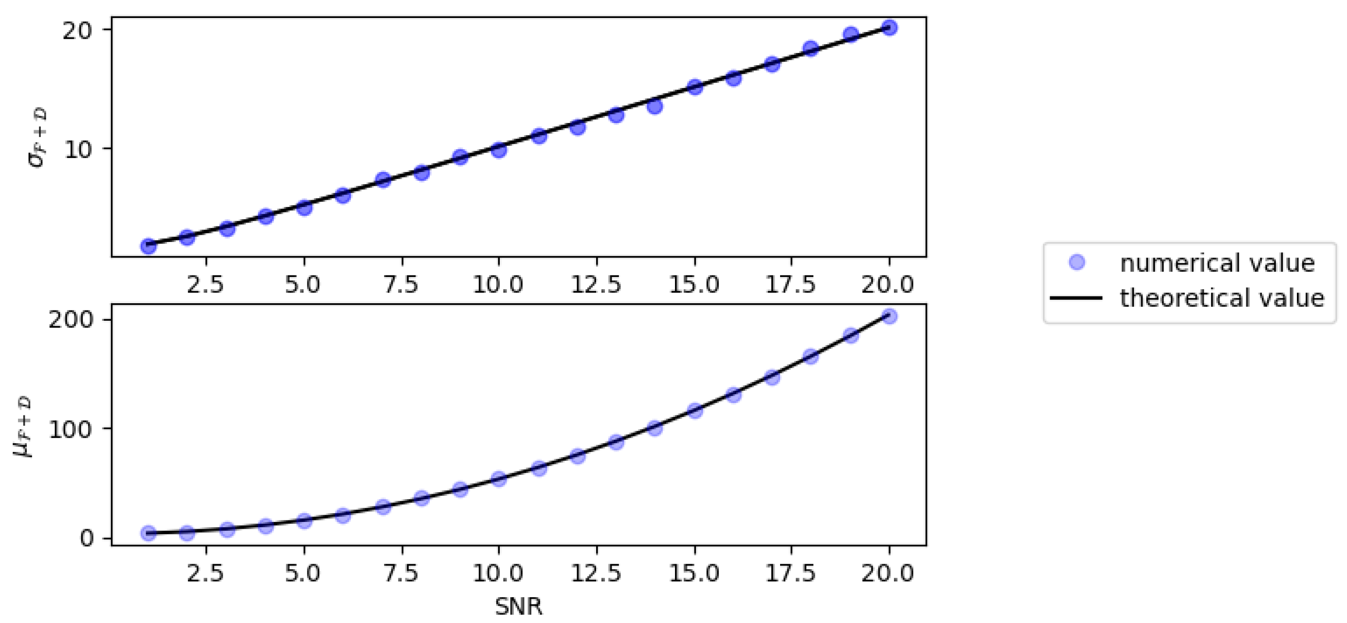
Figure 1 shows the plots of the means and standard deviations of the $\mathcal{D}$-statistic and the $\mathcal{F}$- statistic against the signal-to-noise ratio of the signals added, whereas Figure 2 shows the sum of $\mathcal{D}$ and $\mathcal{F}$ statistics. We compare the simulated values with the theoretical predictions. In Gaussian noise, the $2\times \mathcal{F}$-statistic has the non-central ${\chi }^2$ distribution with 4 degrees of freedom and non-centrality parameter equal to ${\rho }^2$, whereas $2\times \mathcal{D}$-statistic has the non-central ${\chi }^2$ distribution with 2 degrees of freedom. For any non-central ${\chi }^2$ distribution with k independent degrees of freedom, the mean ($\mu$) and standard deviations ($\sigma$) are given by

$$\mu =k+\lambda$$

(141)

and

$$\sigma =\sqrt{2(k+2\lambda )}$$

(142)

where $\lambda$ is the non-centrality parameter. In our case, $\lambda ={\rho }^2$, where $\rho$ is the signal-to-noise ratio defined by Equation (99).

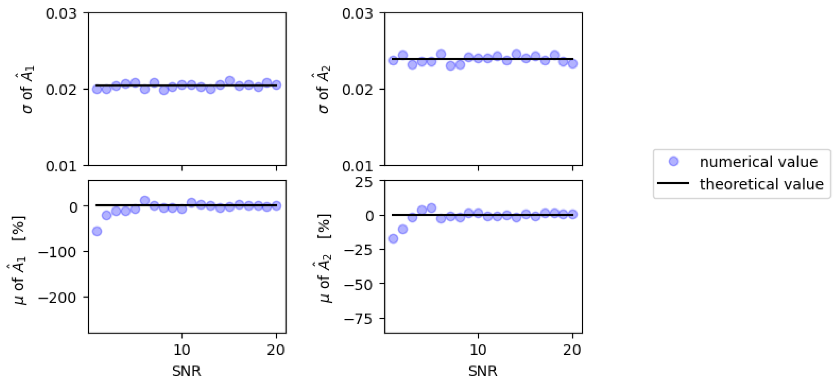
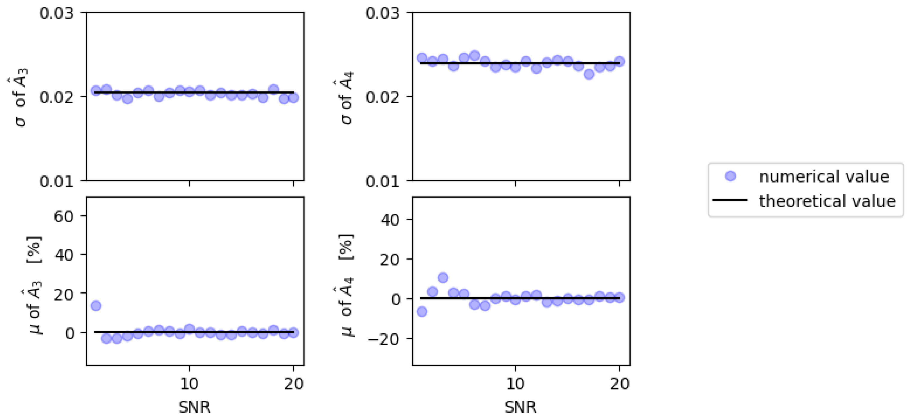
For the case of amplitude parameters, we calculate biases and variances of the parameter estimators and compare them with the theoretical values. For a parameter, the numerical bias is calculated as $\frac{\mathrm{numerical}\mathrm{value}-\mathrm{theoretical}\mathrm{value}}{\mathrm{theoretical}\mathrm{value}}\times 100$. The theoretical biases of parameter estimators are zero, whereas the variances are square roots of the diagonal elements of the inverse of the Fisher matrix given by Equation (102). Figure 3 and Figure 4 show the biases and standard deviations of the estimators of the four quadrupole amplitudes.

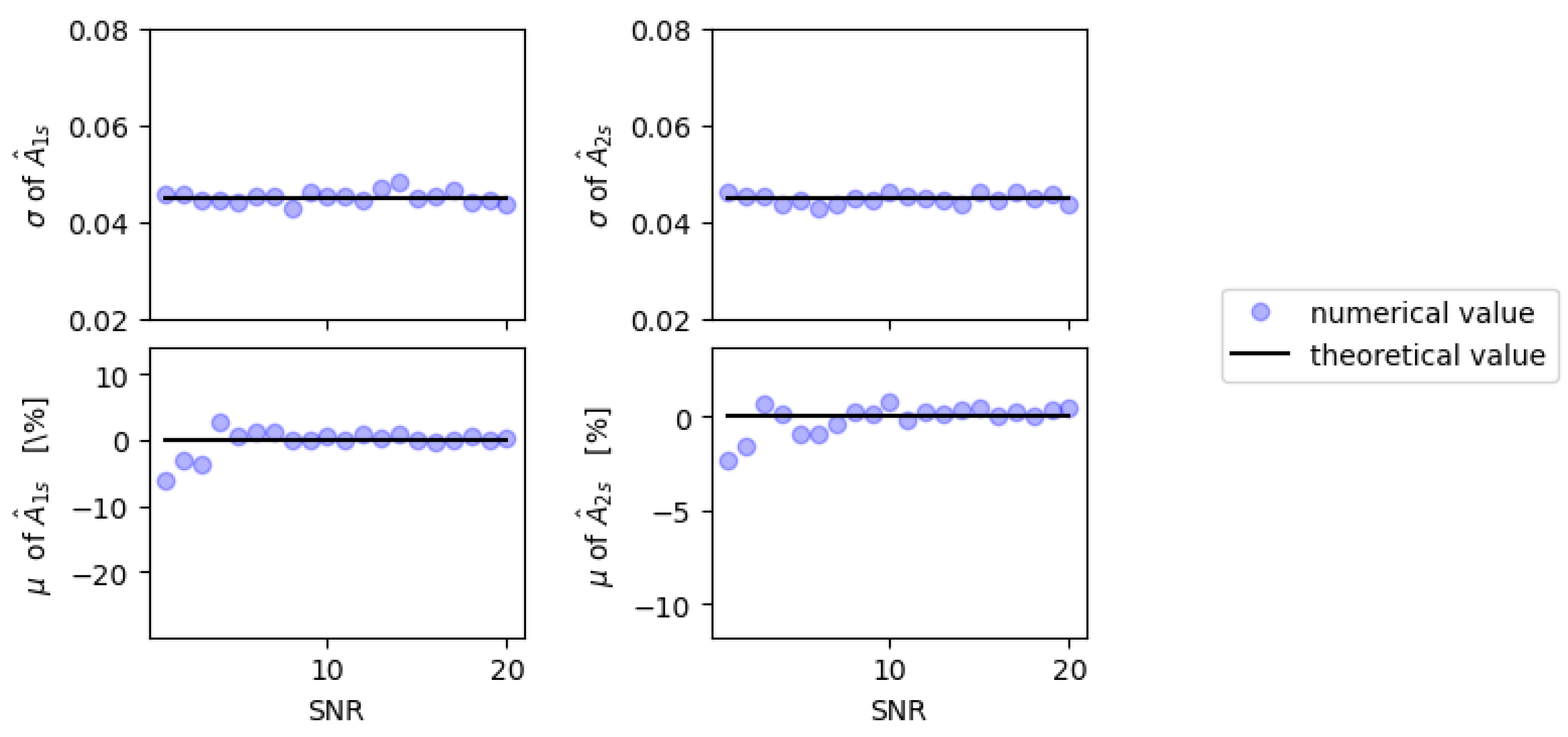
In Figure 5, we present the bias and standard deviation of the estimators of two amplitudes from the dipole radiation.

From our simulations, we also estimate the five astrophysical parameters $\mathit{\theta }=(h_o,h_o^d,\psi ,\iota ,{\varphi }_o)$ using the least squares procedure presented in the previous section. The theoretical estimates of the standard deviation can be obtained from the Fisher matrix $\mathsf{\Gamma }\left(\mathit{\theta }\right)$ for the astrophysical parameters, which is given by the following formula

$$\mathsf{\Gamma }\left(\mathit{\theta }\right)=J^T·\mathsf{\Gamma }\left(\mathcal{A}\right)·J$$

(143)

where $\mathsf{\Gamma }\left(A\right)$ is the Fisher matrix for the amplitude parameters given by Equation (102) and J is the $6\times 5$ Jacobi matrix with elements $J_{lm}=\frac{\partial A_l}{\partial {\mathit{\theta }}_m}$ ($l\in [1,6]$ and $m\in [1,5]$).

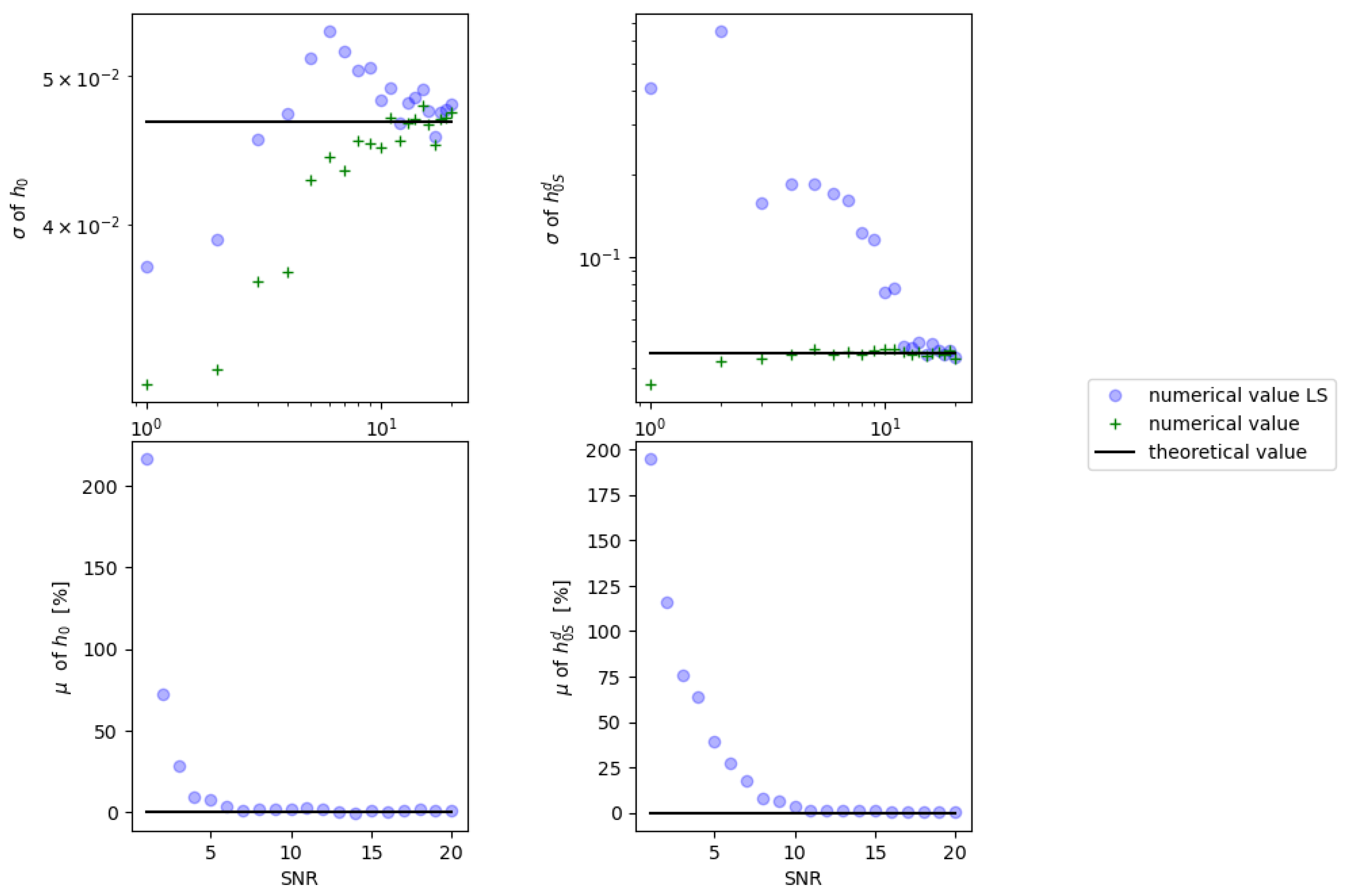
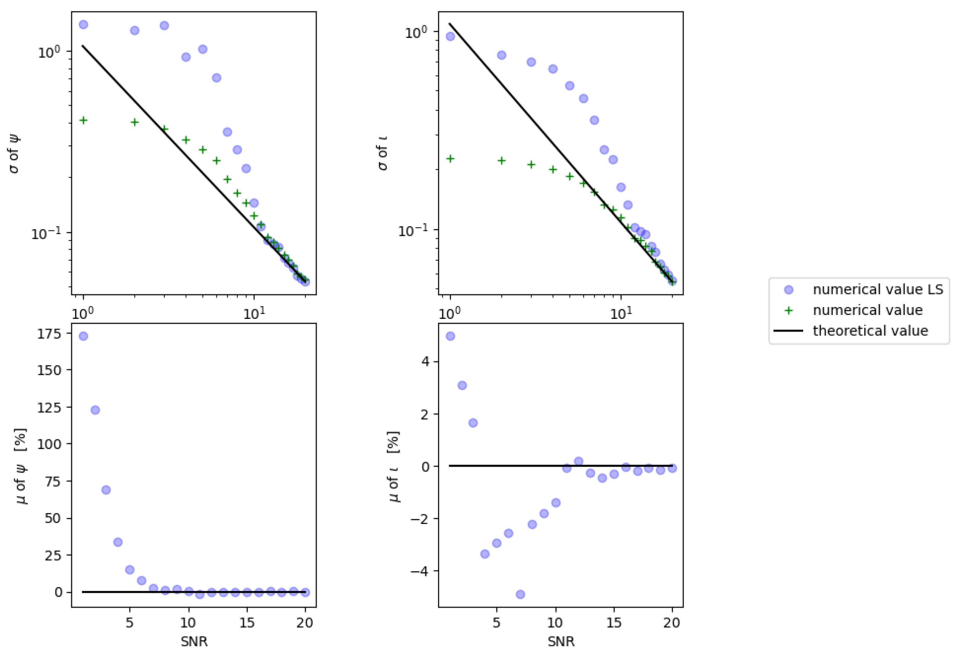
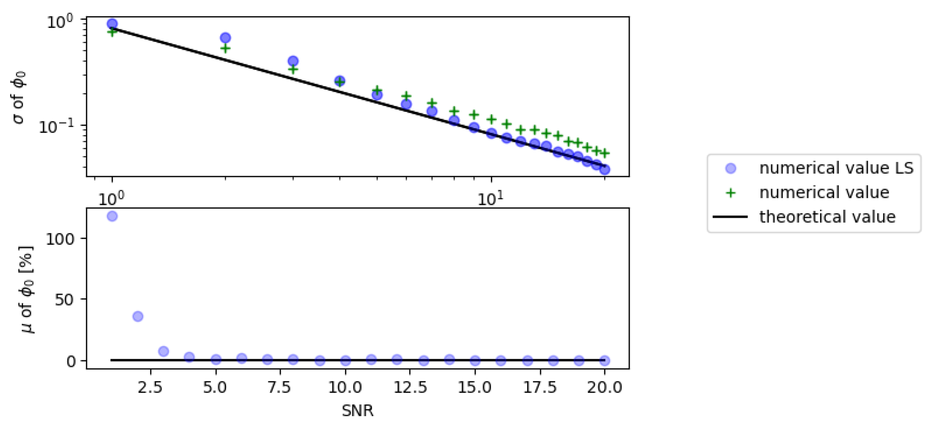
Figure 6, Figure 7 and Figure 8 present the biases and standard deviations of the five astrophysical parameters. We have plotted the theoretical mean and standard deviation against the initial estimators and estimators obtained from the LS procedure.

The astrophysical parameters are related to amplitude parameters by non-linear transformation; consequently, we can expect that their estimators will be unbiased and minimum variance only asymptotically, for a large signal-to-noise ratio. Moreover, the estimators obtained from the LS procedure agree well with the theoretical predictions.

4.3. Conclusions

In this paper, we have derived the response of a laser interferometric detector to a GW signal from a non-axisymmetric rotating neutron star in the BD theory. We have also obtained the maximum likelihood ratio statistic to detect such a signal in the detector data and estimate its parameters. We find that in the Brans–Dicke theory, a non-negligible contribution to gravitational radiation from a rotating neutron star can come from the time-varying dipole moment. We have proposed a scheme whereby detecting both the quadrupole and the dipole radiation, we can estimate the GW amplitude of dipole radiation in the BD theory. We have performed Monte Carlo simulations in white Gaussian noise, which indicate that our scheme detects the signal and estimates its parameters with the theoretically predicted efficiency and accuracy.

References

1. Brans, C.; Dicke, R.H. Mach’s Principle and a Relativistic Theory of Gravitation. Phys. Rev. Lett. 1961, 124, 925. [Google Scholar] [CrossRef]
2. Jordan, P. Zum gegenwärtigen Stand der Diracschen kosmologischen Hypothesen. Z. Phys 1959, 157, 112–121. [Google Scholar] [CrossRef]
3. Fierz, M. Über die physikalische Deutung der erweiterten Gravitationstheorie P. Jordans. Helv. Phys. Acta 1956, 29, 128–134. [Google Scholar]
4. Bertolami, O.; Martins, P.J. Nonminimal coupling and quintessence. Phys. Rev. D 2000, 61, 064007. [Google Scholar] [CrossRef] [Green Version]
5. Will, C.M. The Confrontation between General Relativity and Experiment. Living Rev. Relativ. 2014, 17, 4. [Google Scholar] [CrossRef] [Green Version]
6. Poisson, E.; Will, C.M. Gravity Newtonian, Post-Newtonian, Relativistic; Cambridge University Press: Cambridge, UK, 2014. [Google Scholar]
7. Misner, C.W.; Thorne, K.S.; Wheeler, J.A. Gravitation; W. H. Freeman and Company: San Francisco, CA, USA, 1973. [Google Scholar]
8. Lebach, D.E.; Corey, B.E.; Shapiro, I.I.; Ratner, M.I.; Webber, J.C.; Rogers, A.E.E.; Davis, J.L.; Herring, T.A. Measurement of the Solar Gravitational Deflection of Radio Waves Using Very-Long-Baseline Interferometry. Phys. Rev. Lett. 1995, 75, 1439. [Google Scholar] [CrossRef] [PubMed]
9. Fomalont, E.; Kopeikin, S.; Lanyi, G.; Benson, J. Progress in Measurements of the Gravitational Bending of Radio Waves Using the VLBA. Astrophys. J. 2009, 699, 1395. [Google Scholar] [CrossRef] [Green Version]
10. Shapiro, S.S.; Davis, J.L.; Lebach, D.E.; Gregory, J.S. Measurement of the Solar Gravitational Deflection of Radio Waves using Geodetic Very-Long-Baseline Interferometry Data, 1979–1999. A&A 2009, 499, 1. [Google Scholar]
11. Lambert, S.B.; Le Poncin-Lafitte, C. Determining the relativistic parameter γ using very long baseline interferometry. A&A 2009, 499, 331–335. [Google Scholar]
12. Lambert, S.B.; Le Poncin-Lafitte, C. Improved determination of γ by VLBI. A&A 2011, 529, A70. [Google Scholar]
13. Bertotti, B.; Iess, L.; Tortora, P. A test of general relativity using radio links with the Cassini spacecraft. Nature 2003, 425, 374–376. [Google Scholar] [CrossRef]
14. Konopliv, A.S.; Asmar, S.W.; Folkner, W.M.; Karatekin, O.; Nunes, D.C.; Smrekar, S.E.; Yoder, C.F.; Zuber, M.T. Mars high resolution gravity fields from MRO, Mars seasonal gravity, and other dynamical parameters. Icarus 2011, 211, 401–428. [Google Scholar] [CrossRef]
15. Pitjeva, E.V. Relativistic Effects and Solar Oblateness from Radar Observations of Planets and Spacecraft. Astron. Lett. 2005, 31, 340–349. [Google Scholar] [CrossRef]
16. Vijaykumar, A.; Kapadia, S.J.; Ajith, P. Constraints on the Time Variation of the Gravitational Constant Using Gravitational Wave Observations of Binary Neutron Stars. Phys. Rev. Lett. 2021, 126, 141104. [Google Scholar] [CrossRef] [PubMed]
17. Córsico, A.H.; Althaus, L.G.; Berro, E.G.; Romero, A.D. An independent constraint on the secular rate of variation of the gravitational constant from pulsating white dwarfs. JCAP 2013, 2013, 32. [Google Scholar] [CrossRef]
18. Nordtvedt, K., Jr. Equivalence Principle for Massive Bodies. I. Phenomenology. Phys. Rev. D 1968, 169, 1014. [Google Scholar] [CrossRef]
19. Thorne, K.S.; Dykla, J.J. Black Holes in the Dicke-Brans Theory of Gravity. Astrophys. J. Lett. 1971, 166, L35–L38. [Google Scholar] [CrossRef]
20. Freire, P.C.C.; Wex, N.; Esposito-Farése, G.; Verbiest, J.P.W.; Bailes, M.; Jacoby, B.A.; Kramer, M.; Stairs, I.H.; Antoniadis, J.; Janssen, G.H. The relativistic pulsar–white dwarf binary PSR J1738+0333 – II. The most stringent test of scalar–tensor gravity. MNRAS 2012, 423, 3328. [Google Scholar] [CrossRef]
21. Bhat, N.D.R.; Bailes, M.; Verbiest, J.P.W. Gravitational-radiation losses from the pulsar white-dwarf binary PSR J1141 6545. Phys. Rev. D 2008, 77, 124017. [Google Scholar] [CrossRef]
22. Abbott, B.P.; Abbott, R.; Abbott, T.D.; Acernese, F.; Ackley, K.; Adams, C.; Adams, T.; Addesso, P.; Adhikari, R.X.; Adya, V.B. Tests of General Relativity with GW170817. Phys. Rev. Lett. 2019, 123, 011102. [Google Scholar] [CrossRef] [Green Version]
23. Riles, K. Recent searches for continuous gravitational waves. Mod. Phys. Lett. A 2017, 32, 1730035. [Google Scholar] [CrossRef]
24. Aasi, J.; Abbott, B.P.; Abbott, T.; Abernathy, M.R.; Ackley, K.; Adams, C.; Adams, T.; Addesso, P.; Adhikari, R.X.; Adya, V.; et al. Advanced LIGO. Class. Quantum Grav. 2015, 32, 074001. [Google Scholar]
25. Acernese, F.; Agathos, M.; Agatsuma, K.; Aisa, D.; Allemandou, N.; Allocca, A.; Amarni, J.; Astone, P.; Balestri, G.; Ballardin, G.; et al. Advanced Virgo: a second-generation interferometric gravitational wave detector. Class. Quantum Grav. 2015, 32, 024001. [Google Scholar] [CrossRef] [Green Version]
26. Akutsu, T.; Ando, M.; Arai, K.; Arai, Y.; Araki, S.; Araya, A.; Aritomi, N.; Aso, Y.; Bae, S.; Bae, Y.; et al. Overview of KAGRA: Detector design and construction history. arXiv 2005, arXiv:2005.05574. [Google Scholar]
27. Abbott, B.P.; Abbott, R.; Acernese, F.; Ackley, K.; Adams, C.; Adams, T.; Addesso, P.; Adhikari, R.X.; Adya, V.B.; Affeldt, C.; et al. First Search for Nontensorial Gravitational Waves from Known Pulsars. Phys. Rev. Lett. 2018, 120, 031104. [Google Scholar] [CrossRef] [PubMed] [Green Version]
28. Isi, M.; Pitkin, M.; Weinstein, A.J. Probing Dynamical Gravity with the Polarization of Continuous Gravitational Waves. Phys. Rev. D. 2017, 96, 042001. [Google Scholar] [CrossRef] [Green Version]
29. Królak, A.; Jaranowski, P. Analysis of Gravitational-Wave Data; Cambridge University Press: Cambridge, UK, 2009. [Google Scholar]
30. Jaranowski, P.; Królak, A.; Schutz, B.F. Data analysis of gravitational-wave signals from spinning neutron stars: The signal and its detection. Phys. Rev. D 1998, 58, 063001. [Google Scholar] [CrossRef] [Green Version]
31. Abbott, R.; Abbott, T.D.; Abraham, S.; Acernese, F.; Ackley, K.; Adams, A.; Adams, C.; Adhikari, R.X.; Adya, V.B.; Affeldt, C.; et al. Gravitational-wave Constraints on the Equatorial Ellipticity of Millisecond Pulsars. Astrophys. J. Lett. 2020, 902, L21. [Google Scholar] [CrossRef]
32. Abbott, B.P.; Abbott, R.; Abbott, T.D.; Abraham, S.; Acernese, F.; Ackley, K.; Adams, C.; Adhikari, R.X.; Adya, V.B.; Affeldt, C.; et al. Narrow-band search for gravitational waves from known pulsars using the second LIGO observing run. Phys. Rev. D 2019, 2002. [Google Scholar] [CrossRef] [Green Version]
33. Abbott, B.P.; Abbott, R.; Abbott, T.D.; Abernathy, M.R.; Acernese, F.; Ackley, K.; Adams, C.; Adams, T.; Addesso, P.; Adhikari, R.X.; et al. First Search for Gravitational Waves from Known Pulsars with Advanced LIGO. Astrophys. J. 2017, 839, 12. [Google Scholar] [CrossRef]
Figure 1. Simulated mean μ and standard deviation σ of the F -statistic (left panels) and the D -statistic (right panel) for an array of SNRs. Continuous lines are the theoretical predictions.
Universe 07 00235 g001
Figure 2. Simulated mean μ and standard deviation σ of the sum of F -statistic and D -statistic for an array of SNRs. Continuous lines are the theoretical predictions.
Universe 07 00235 g002
Figure 3. Bias and standard deviation of the quadrupole amplitudes A 1 (left panel) and A 2 (right panel). Theoretical predictions are drawn as continuous lines.
Universe 07 00235 g003
Figure 4. Bias and standard deviation of the quadrupole amplitudes A 3 (left panel) and A 4 (right panel). Theoretical predictions are drawn as continuous lines.
Universe 07 00235 g004
Figure 5. Bias and standard deviation of dipole amplitudes: A 1 S (left) and A 2 S (right).
Universe 07 00235 g005
Figure 6. Bias and standard deviation of estimators of the two amplitude parameters h o (left panels) and h o d (right panels). The crosses are for initial estimators obtained from the Equations (136) and (139) and the dots are for the estimators from the least-squares procedure. Continuous lines are theoretical predictions from the Fisher matrix. The standard deviation is a log-log plot.
Universe 07 00235 g006
Figure 7. Bias and standard deviation of estimators of angles ψ (left panels) and ι (right panels). The crosses are for initial estimators obtained from the Equations (137) and (138) and the dots are for the estimators from the least-squares procedure. Continuous lines are theoretical predictions from the Fisher matrix. The standard deviation is a log-log plot.
Universe 07 00235 g007
Figure 8. Bias and standard deviation of phase angle ϕ o . The crosses are for initial estimators obtained from the Equation (140) and the dots are for the estimators from the least-squares procedure. Continuous lines are theoretical predictions from the Fisher matrix. The standard deviation is a log-log plot.
Universe 07 00235 g008
Publisher’s Note: MDPI stays neutral with regard to jurisdictional claims in published maps and institutional affiliations.