Article

Lensing Magnification Seen by Gravitational Wave Detectors

1
Centre for Astroparticle Physics, Département de Physique Théorique, Université de Genève, 24 quai Ernest-Ansermet, 1211 Geneva, Switzerland
2
Institut d’Astrophysique de Paris, Sorbonne Université, CNRS, UMR 7095, 98 bis Boulevard Arago, 75014 Paris, France
*
Author to whom correspondence should be addressed.
Universe 2022, 8(1), 19; https://doi.org/10.3390/universe8010019
Submission received: 26 November 2021 / Revised: 17 December 2021 / Accepted: 20 December 2021 / Published: 30 December 2021
(This article belongs to the Special Issue Gravitational Radiation in Cosmological Spacetimes)

Abstract

:
In this paper, we studied the gravitational lensing of gravitational wave events. The probability that an observed gravitational wave source has been (de-)amplified by a given amount is a detector-dependent quantity which depends on different ingredients: the lens distribution, the underlying distribution of sources and the detector sensitivity. The main objective of the present work was to introduce a semi-analytic approach to study the distribution of the magnification of a given source population observed with a given detector. The advantage of this approach is that each ingredient can be individually varied and tested. We computed the expected magnification as both a function of redshift and of the observedsource luminosity distance, which is the only quantity one can access via observation in the absence of an electromagnetic counterpart. As a case study, we then focus on the LIGO/Virgo network and on strong lensing ( μ > 1 ).

1. Introduction

The direct detection of gravitational waves (GWs) from inspiraling binary black holes and neutron stars by the LIGO and Virgo experiments [1,2,3,4,5,6,7,8,9,10,11] has been one of the greatest successes in experimental physics and observational astronomy in recent years. Not only did it lead to unprecedented insights into black holes and especially neutron stars, but it also allowed us to test general relativity (GR) and cosmology.
An interesting aspect is the fact that the clustered matter between the gravitational wave source and the observer can amplify the observed signal. This may lead to an underestimation of the distance to the source and therefore of its redshift which in turn leads to an overestimation of the chirp mass [12]. The effects of gravitational lensing on the apparent properties of detected sources and the possible identification of unique lensing features were extensively studied [13,14,15,16,17,18,19,20,21,22,23,24,25,26,27,28]. The prospects of the lensing of gravitational waves alone or in combination with other data as a probe of dark matter or of general relativity have also been investigated [29,30,31,32].
In this paper, we sought to determine the probability that an event of a given strain amplitude, or rather of a given signal-to-noise ratio (SNR) for fixed experimental characteristics, is being significantly magnified by lensing. In particular, we studied the dependence of the lensing probability and of the mean magnification on redshift and on the strain amplitude (or SNR). Similar studies were already present in the literature [12,15,18,25,26,33,34,35]. The main difference with the present work is that, instead of full numerical simulations with ray tracing, we presented semi-analytic formulae which can be applied to an arbitrary lens and source distribution, maintaining full control of the modeling and transparency of all physical effects. This allowed us to study the dependence of the result on the lens and/or source distribution which is otherwise quite obscure. Our analysis can also be easily adapted to an arbitrary experiment given the expected number of sources as a function of their SNR and redshift. Moreover, unlike previous studies on this subject, we compute the expected magnification as a function of redshift, but also as a function of the observed luminosity distance, which is the only quantity one can access observationally in the absence of an electromagnetic counterpart. While in principle it is possible to determine the redshift of an inspiraling binary black hole from the light curve, the LIGO/Virgo observations have by far too large error bars to do this. Here, we assume the Planck concordance cosmology to determine the redshift from the luminosity distance. If lensing is relevant, this redshift is, however, not correct, as the inferred distance is affected by lensing. The advantage of having a semi-analytic analysis is that it allows us to answer the question of whether it is feasible that some or most of the observed LIGO/Virgo events are strongly lensed, as proposed in [16,17,27,36]. We show that, in order to achieve a significant lensing probability for more than one of these events, one has to tweak the lens and source distribution in a way that is in contradiction with the present observational constraints and with results from simulations.
In this work, we focus on strong lensing. We are indeed interested in working out the distribution of magnification μ > 1 for sources visible by LIGO/Virgo/Kagra. The magnification induced by a cosmological large scale-structure, which can also lead to de-magnification, μ < 1 , is negligible for this study. For the distances of the LIGO/Virgo sources, it only leads to small corrections to the results presented herein. We modeled the lenses as singular isothermal spheres (SISs) which is reasonable for galaxies. While SISs are not realistic when considering lensing by individual clusters, they are roughly sufficient for statistical purposes, as can be seen in the detailed study of [37,38]. The main advantage of SISs is of course that they allow for analytic results. Note that we are only interested in the magnification of the strongest image and not in the more detailed structure of the lensing event such as the time delays or the relative strength of images.
We concentrate on transient sources, such as compact binary coalescences which can be observed with LIGO/Virgo/Kagra [1,2,3,4,5,6,8,9,10,11]. The degeneracy between the intrinsic chirp mass and redshift of such systems may pose interesting questions. Many of the binary black holes (BBHs) detected by LIGO/Virgo are much more massive than those known from X-ray binaries in the galaxy (the latter have masses only up to ∼ 25 M ) and in some cases, BBHs detected in GW have masses well above 60 M [6,8]. Black hole (BH) masses above ∼ 25 M are expected in low-metallicity environments and are indeed predicted by various stellar evolution models (e.g., [39,40,41,42,43,44,45,46,47,48]). However, standard stellar evolution models struggle to explain masses in the so-called ’pair-instability mass gap’ in the range between ∼ 60 M and ∼ 130 M , where no BHs are expected to form [49]. An intriguing possibility could be that the apparent high masses are the result of redshifting, implying that at least some of the observed BBHs are high-redshift sources with low intrinsic masses that underwent significant gravitational lensing [16].
A detailed analysis of the individual events in Ref. [33] concluded that the probability of lensing for the sources observed by LIGO/Virgo runs O(1) and O(2) is vanishingly small, with the consequence that BH population models can be reasonably informed by GW observations to date [8,11,50]. In this work, we confirmed this finding with a statistical analysis. We present predictions for the probability that an event observed by LIGO/Virgo at a given distance has been magnified by a given amount: while the probability for more than one event is very small (the probability that two events are magnified by more than a factor 5 is approximately 10 10 for the typical distances of LIGO/Virgo events), it slowly decays with increasing magnification, i.e., there is a non-negligible probability of having extremely highly magnified events (the probability that an event at a distance larger than 2500 Mpc is magnified by a factor of more than 100 is approximately 10 7 ).
The remainder of this paper is structured as follows. In the next section, we present the lens model and we derive expressions for the cross-section, optical depth and lensing probability for a distribution of lenses. The results presented in this section are not new. The optical depth for strong lensing was already derived in the pioneering works of Turner et al. and later by Fukugita et al. and Oguri et al. [51,52,53]. Probability distributions for different lensing properties were derived from numerical N-body simulations in [54,55]. Our results are in agreement with this work. In Section 3, we derive the expression for the probability that a source seen from a given observed distance was magnified by a given factor and we compute the mean magnification and its variance both as a function of the (unobservable) cosmological redshift and the observed distance which can be converted into an ‘apparent’ redshift under the assumption of Λ CDM cosmology with Planck values for the cosmological parameters. In Section 4, we introduce a numerical study for the population of lenses and sources and we present numerical results for the magnification as a function of both cosmological and observed redshift, for the LIGO/Virgo detector network. We also compute the probability of magnification for a source with given observed properties. In Section 5, we discuss our results and conclude. In a series of appendices, we discuss a simple analytical model which is useful to understand the physics and we present results for the mean magnification for different choices of source distribution.
Notation: In this paper, we set c = 1 but keep the gravitational constant G. We define θ and β as the lensed and the unlensed angular position of the source. The optical axis connects the observer to the center of mass of the lens. We introduce a vector in the source plane from the optical axis to the source, b = d s β and a vector ξ in the lens plane defined as ξ = θ d . This fixes the geometry. Here, d = d ( z ) , d s = d ( z , z s ) and d s = d ( z s ) are the angular diameter distances from the observer to the lens, from the lens to the source and from the observer to the source, respectively. These quantities are illustrated in Figure 1. A glossary with a list of the main symbols introduced in this article and their corresponding definitions can be found in Table 1.

2. Lens Modeling

We describe galaxies acting as lenses as singular isothermal spheres and we derive expressions for the magnification between multiple images as a function of the geometrical quantities entering the picture. Most of this section follows Refs. [51,52,56]. SISs are not a very realistic lens model but since we are interested in statistical averages and not in the detailed modeling of a single lens, the fact that individual lenses will in general be triaxial is expected to average out. Furthermore, the neglected substructure may actually lead to some additional magnification. In this sense, our model is rather conservative. However, a recent numerical study has shown that the SIS model is surprisingly close to the observed lensing probability [38]. Note also that our results are only sensitive to the magnification of the most highly magnified image but not to the geometry or the number of images.

2.1. Basic Strong Lensing Quantities

The matter density of a singular isothermal sphere is given by
ρ ( r ) = σ v 2 2 π G r 2 ,
where σ v denotes the velocity dispersion of the lens. Despite the singularity in the center and the infinite total mass, this can be considered as a rather realistic mass distribution for lensing by a galaxy (see [34,56]), where σ v is the velocity dispersion inside the galaxy. Integrating along the line of sight, we obtain the surface density:
Σ ( θ ) = σ v 2 2 G 1 d θ .
We introduce Σ c = ( 4 π G ) 1 d s / ( d s d ) so that the convergence κ is given by
κ ( θ ) = Σ ( θ ) Σ c = 2 π σ v 2 d s d s 1 θ .
An SIS has a constant deflection angle given by
α ( θ ) = 4 π σ v 2 d s d s = 2 θ κ ( θ ) α 0 .
We now rescale our variables by α 0 , defining the rescaled image and source positions as x = θ / α 0 and y = β / α 0 , respectively. In terms of these rescaled variables, the lens equation for the SIS simply becomes y = x x / | x | . For y = 0 , the solution is the Einstein ring | x | = 1 , and for y = | y | < 1 , there are two solutions: one with x 1 = | x 1 | = 1 + y on the same side of the line of sight as the source (positive parity); and one with x 2 = | x 2 | = 1 y on the opposite side (negative parity). For y > 1 , the second solution no longer exists. The Jacobian of the lens map is:
A i j = δ i j 1 1 | x | + x i x j | x | 3 , det A = 1 1 | x | , μ = 1 | det A | = | x | | 1 | x | | ,
where we introduced the magnification μ . Expressing the total magnification of a point source at position y in terms of y, we find:
μ ( y ) = μ ( x 1 ) + μ ( x 2 ) = y + 1 y + 1 y y = μ 1 + μ 2 = 2 y , y 1 , y + 1 y = 1 + 1 y , y 1 .

2.2. Optical Depth and Lensing Probability

The impact parameter of the source (in the source plane) is given by | b | = b = β d s = y α 0 d s . A source with an impact parameter smaller or equal to b was amplified by a factor of at least μ ( y ) . Hence, the cross-section for amplification by more than a factor of μ 1 of the stronger image from a SIS lens with velocity dispersion σ v is:
σ ( μ 1 , z , z s , σ v ) = π b 2 = π ( y α 0 d s ) 2 = π ( 4 π ) 2 σ v 4 d s 2 ( μ 1 1 ) 2 .
Note that this cross-section gives the area, centered along the line of sight of the lens, within which a source at z s must lie so that it is amplified by a factor μ 1 or larger by the lens at z . Expression (7) also remains valid for y 1 , where we have only one image with magnification μ 1 which tends to 1 when y .
In our study of the strong lensing of gravitational waves, we only considered one image and not the sum of both since we expect to see a short burst of GWs which only comes from one image. The second image is delayed in time, with a typical time delay of the order of a few months (as can be seen in, e.g., [12]), which is much longer than the GW burst. Since we are interested in magnification, we shall compute the cross-section for the stronger image. This point has been neglected in the previous literature: in Equation (7), y 1 = μ 1 1 is usually replaced by y 1 = μ / 2 = ( μ 1 + μ 2 ) / 2 which is the correct expression for a static situation in which both images are seen together. For strong amplification, μ 1 μ 2 1 —a difference which reduces the cross-section by a factor of 4.
To compute the optical depth to the source of magnification by at least μ , denoted by τ ( μ , z s ) , we need to know the physical density n ( σ v , z ) of lenses (galaxies) with a given velocity dispersion σ v at redshift z . We define the density function n ( σ v , z ) such that its integral n ( σ v , z ) d σ v simply gives the total density of lenses at redshift z .
The optical depth for lensing with magnification μ (of the most strongly magnified image in the case of two images) for a source at redshift z s is:
τ ( μ , z s ) = 0 z s d z d r d z d d s 2 σ ( μ , z , z s , σ v ) n ( σ v , z ) d σ v ,
where d r is the physical length element at redshift z . Note also that we rescaled the cross-section to the lens redshift, σ σ ( d / d s ) 2 , since in Equation (8), we multiply by the lens density at z . Inserting this and (7) for the cross-section in Equation (8), we obtain:
τ ( μ , z s ) = = π ( 4 π ) 2 ( μ 1 ) 2 0 z s d z χ 2 ( z , z s ) χ 2 ( z ) χ 2 ( z s ) ( 1 + z ) 3 H ( z ) 0 d σ v σ v 4 n ( σ v , z ) ,
where χ ( z 1 , z 2 ) denotes the co-moving distance from the redshift z 1 to z 2 and χ ( z ) = χ ( 0 , z ) . Equation (9) is the optical depth for magnification larger than  μ .
Often, only the strong lensing case is considered and the magnification from the two images is added to give the total magnification. To do this, one has to replace 1 / ( μ 1 ) 2 by 4 / μ 2 . As already mentioned above, we cannot do this herein since in the case of strong magnification and double images, we expect a considerable time delay, so that typically, we observe only one image at one given time. Here, we assume this to be the stronger image. In the strong magnification case, μ 2 , this difference is roughly a factor 4, while in the limit y 1 where μ 2 and the second image disappears, the two expressions agree.
The probability of having an event from redshift z s magnified by more than μ is:
P ( > μ , z s ) = 1 exp ( τ ( μ , z s ) ) = μ p ( μ , z s ) d μ ,
where p ( μ , z s ) is the probability density for magnification by μ :
p ( μ , z s ) = d d μ P ( > μ , z s ) = d τ d μ exp ( τ ( μ , z s ) ) .
To understand Equation (10), note that d τ / d z is the scattering rate leading to a magnification larger than μ (per redshift). Hence the probability for magnification larger than μ satisfies the differential equation d P ( > μ , z ) / d z = ( 1 P ) d τ / d z with solution (10). The factor ( 1 P ) is essential to keep the probability normalized also when τ becomes large. In the limit of small optical depth, P ( > μ , z s ) = τ ( μ , z s ) .
Note that, while our formula also holds if there is only one image, μ < 2 , it cannot describe the de-magnification which happens when a beam (from a GW or a light source) crosses an under-density. An SIS is always an over-density. Therefore, our formulas are restricted to μ > 1 .
The probability density and probability defined in this section only depend on the lens model and lens distribution but not on the distribution of sources or on the sensitivity of the instrument. They are detector-independent functions which depend on the cosmological source redshift, which is a quantity that cannot be accessed observationally (without assuming the existence of an optical counterpart) as it is degenerate with the (unknown) magnification. The physically interesting quantity is rather the probability that a source that we observe from a given observed distance has been magnified by a given amount. We introduced this quantity in the next section and we will see that it depends on both the distribution of sources and the specifications of a given instrument.

3. Inclusion of Lensing Selection Effects

In this section, we derive expressions for the probability that a given source observed from a given distance has a magnification μ , as a function of both redshift and observed source distance. Several ingredients enter the computation: the probability distribution of magnification given a lens population p ( μ , z ) given by Equations (9) and (11), the underlying source population and the sensitivity curve of a given instrument. As an instrument has finite sensitivity, highly magnified sources are easier to detect than non-magnified ones: hereafter, we dub these effects lensing selection effects. These results are valid for a generic distribution of magnification p ( μ , z ) , in particular, they also stay valid when one adds weak lensing contribution to the distribution of strong lensing studied in this work. We will come back to this point in the discussion session.

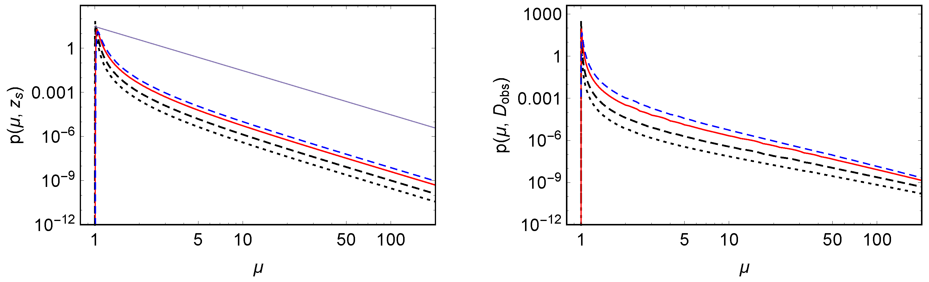
3.1. Magnification Distribution as Function of Redshift

Compact binary coalescences can be detected using matched filtering techniques, where a model of the signal, which depends on the physical parameters of the source, is matched against the observed signal (see [9] for a description and further references). For a given detector sensitivity and a given template bank used to perform the matched filtering, the obtained SNR ρ can be related to a false alarm rate (FAR), which in turn sets a threshold for detection. For example, the O3a LIGO/Virgo catalog [9] includes sources with the FAR below 2 y 1 . For simplicity, we will work directly with a limiting SNR ρ lim and assume that the signal is detected if ρ ρ lim , where the SNR ρ is defined by [57]
ρ 2 = 4 | h ( f ) | 2 S n ( f ) d f = ρ 2 ( f ) d f .
Here, S n ( f ) is the noise of the detector at frequency f, as can be seen in [58].
If an event is magnified by μ > 1 , we observe it even if without magnification, its SNR would have been ρ lim / μ < ρ lim . It follows that in the presence of magnification, the total number of objects which we expect to see from a redshift bin d z is given by the following convolution:
d N obs ( z , ρ lim ) = 0 d μ p ( μ , z ) N ( μ , z ) ,
where p ( μ , z ) is the distribution of lensing magnification as a function of cosmological redshift and:
d N ( μ , z ) d z ρ lim / μ N ( ρ , z ) d ρ ,
is the number of sources that we see from redshift z in the presence of magnification μ . In Equation (14) N ( ρ , z ) is the number density of sources as a function of redshift and ρ . We denote by ρ the SNR of a source computed assuming no lensing effects. The mean amplification of a source at redshift z is:
μ ( z ) = 0 d μ μ p ( μ , z ) d N ( μ , z ) 0 d μ p ( μ , z ) d N ( μ , z ) .
Note that (15) is the first moment of the probability distribution of magnification:
P z ( μ , z ) C p ( μ , z ) d N ( μ , z ) d z ,
where C is a normalization constant. Equation (16) depends on three basic ingredients: (i) distribution of magnification p ( μ , z ) ; (ii) distribution of sources as a function of redshift and luminosity (or analogously ρ ); (iii) sensitivity curve of a given experiment which determines ρ lim .
For sufficiently high μ , p ( μ , z s ) d τ / d μ μ 3 , while the number of sources which we see with magnification μ or more from a redshift bin around z s , defined in Equation (14), becomes independent of μ for large values of μ . Indeed, in the presence of very high magnification, we simply see all sources that are present. This last statement is general and does not depend on the details of the distribution of sources. It follows from the physical assumption that there exists a minimum value for the intrinsic luminosity emitted, L min , and once μ is such that L lim / μ < L min , we see all sources and the luminosity integral no longer depends on μ . The probability of having magnification bigger than μ for a given source redshift is given by the integral of the probability distribution of magnification, Equation (16), from a minimum value μ . We denote this quantity as P z ( > μ ) . For large values of magnification P z ( > μ ) μ 2 , the variance of the distribution, defined by Var ( μ ) μ 2 μ 2 , is log-divergent. We stress that this is a general property of the probability distribution of magnification in strong lensing. It does not depend on the details of the distribution of sources, nor on the details of the lens distribution. Moreover, it also applies to the case of transient electromagnetic sources lensed by galaxies. Of course, this divergence is not physical. When the magnification becomes very large, y is very small and the geometric optics treatment adopted here breaks down. Nevertheless, this indicates that the distribution has a significant tail with large magnification. Even though, as we shall see, the probability for a magnification of, e.g., 10, is very small; it is not exponentially small as it would be for a Gaussian distribution, but it only decays as a mild power law.

3.2. Magnification Distribution as Function of Observed Distance

The functions determined thus far, however, are not observable as we typically do not know the intrinsic cosmological redshift of a GW event. We usually infer it by assuming that the observed luminosity distance is the one of the background universe without magnification. This is of course not true when magnification is relevant. We therefore rewrite (13) and (15) as functions of the observed luminosity distance which is directly extracted from observations. It is given by
D obs ( z s , μ ) D s ( z s ) μ .
The number of sources that we can see from an observed luminosity distance D obs ± d D obs / 2 is obtained from (13), rewriting all quantities as functions of the observed distance and replacing the redshift bin d z s by ( d D obs / d z s ) 1 d D obs = μ ( d D s / d z s ) 1 d D obs . This gives:
d N obs ( D obs , ρ lim ) = 0 d μ p ( μ , z s ( D obs , μ ) ) d N ( μ , D obs ) ,
where:
d N ( μ , D obs ) = d D obs μ D s ( z s ) ρ lim / μ N ( ρ , z s ( D obs , μ ) ) d ρ ,
is the number of sources which we see from a luminosity distance D obs ± d D obs / 2 , with magnification μ . In these expressions, z s ( D obs , μ ) z s ( D s = μ D obs ) is the cosmological redshift that corresponds to the observed distance D obs = μ D s ( z s ) . Not to be confused with the redshift inferred by an observer who assumes that D obs is the luminosity distance of the background universe (without magnification). This latter, which we denote by z obs , is given by D s ( z obs ) = D obs . In Equation (19) D s ( z s ) d D s / d z s . The average amplification as a function of the observed luminosity distance is therefore:
μ ( D obs ) = 0 d μ μ p ( μ , D obs ) d N ( μ , D obs ) / d D obs 0 d μ p ( μ , D obs ) d N ( μ , D obs ) / d D obs ,
which of course depends on the threshold ρ lim , i.e., on the detector sensitivity. In full analogy with Equation (16), we introduce the probability distribution of magnification as a function of the observed luminosity distance of the source:
P obs ( μ , D obs ) C p ( μ , D obs ) d N ( μ , D obs ) d D obs ,
where C is a constant of normalization which is given by the denominator of (20). Equations (13)–(16) and Equations (18)–(21) are the main results of this section.
From Equation (19), it follows that d N ( μ , D obs ) / d D obs μ for μ 1 as both the lower integration bound and D s tend towards constant asymptotic values for large magnification μ . The probability density p ( μ , D obs ) in (21) also depends on μ through the observed luminosity as we defined p ( μ , D obs ) p ( μ , z s ( μ D obs ) ) . Recalling that p ( μ , z s ) μ 3 , it follows that p ( μ , D obs ) will have a milder decay with magnification. Indeed, for a fixed D obs and μ > 1 , p ( μ , D obs ) p ( μ , z s ( μ D obs ) ) also receives contributions from redshifts higher than z s ( D obs ) and therefore the lensing probability is higher. The exact scaling of p ( μ , D obs ) with μ depends on the details of the lens distribution.
We anticipate here some results that we will obtain in Section 4.1 when considering a realistic model for the galaxy distribution and evolution. For a realistic distribution with co-moving number density of lenses which reproduces observations (or hydrodynamical simulations calibrated to observations), we find that p ( μ , D obs ) μ α . The value of α increases from 2 to 3 as we increase the observed luminosity distance from ∼300 Mpc to 5000 Mpc, where it saturates to the asymptotic value α = 3 . It follows that the probability distribution (21) scales as P obs ( μ ) μ α + 1 / 2 and its integral from μ to infinity behaves as P obs ( > μ ) μ α + 3 / 2 for large values of μ . It follows that, for any fixed value of D obs , the variance of the distribution diverges as μ α + 7 / 2 . We stress that this is a general property of the probability distribution of magnification (for different observed redshift), independent from the details of the distribution of sources. Moreover, it also applies to the case of strongly lensed sources of electromagnetic radiation. Furthermore, in that case, the variance of the distribution of magnification (for a given observed redshift or luminosity distance) is divergent. We observed that for realistic models of lens distribution, the mean of (21) also diverges for small observed distances where α 2 . The fact that the variance of the distribution diverges is due to the presence of extremely highly magnified sources, i.e., sources aligned along the lens–observer direction for which the magnification μ , as can be seen in Equation (6). This is also at the origin of the divergence of the mean of the magnification at small observed distances. Physically, the magnification tends to a finite value and as mentioned above, the presence of the divergence is due to the geometric optics approximation, which breaks down in the vicinity of caustics, where wave effects need to be taken into account. The fact that the mean of the magnification diverges only for small observed distances is due to the fact that, if a given source is very highly magnified, it appears to be at a small observed distance D obs . We will get back to this point in Section 4 and Section 5.

4. Numerical Results

In this section, we model the redshift distribution and redshift evolution of lenses (galaxies) using fits to hydrodynamical simulations. We also model the distribution of GW sources using a phenomenological model of the binary BH population. We then compute the distribution of magnification as a function of the cosmological source redshift and of the observed one. We focus on the case of the two LIGO/Virgo detectors.

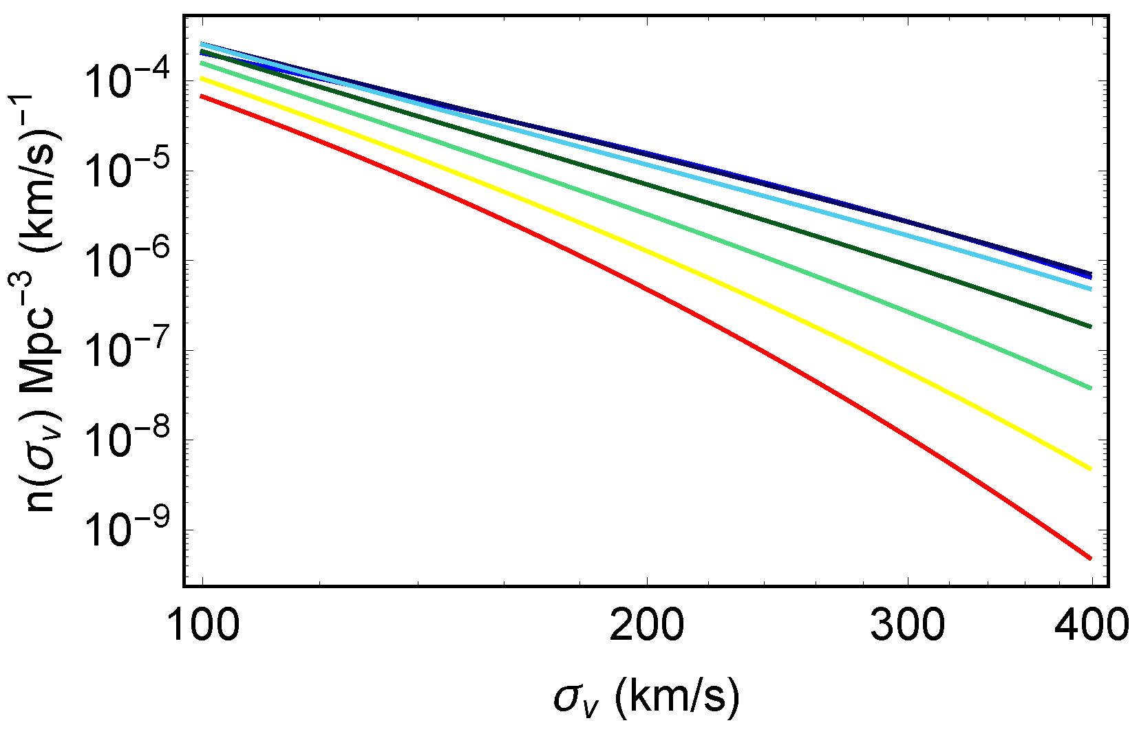
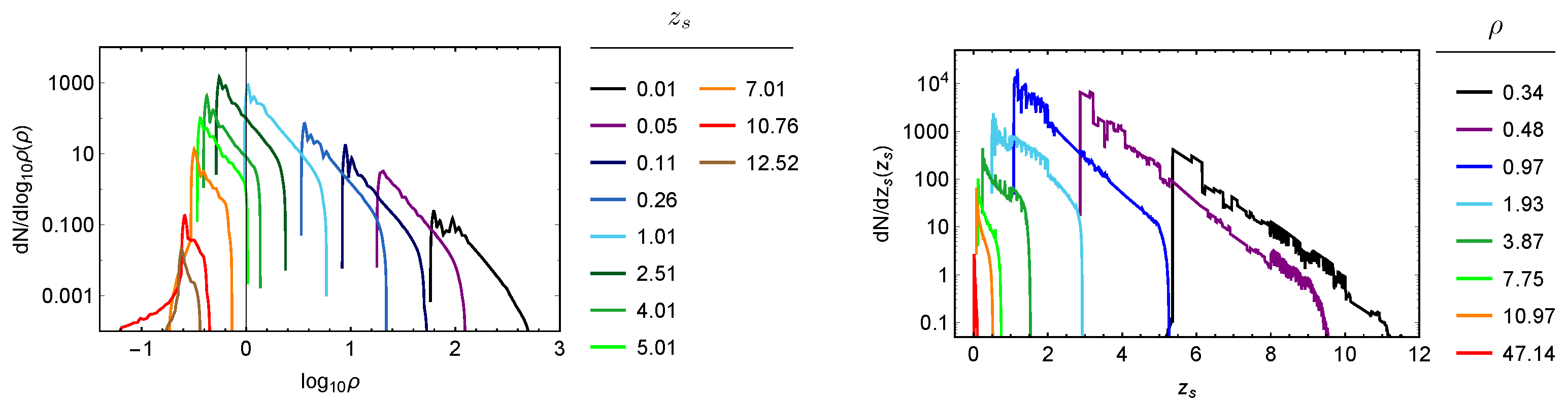
4.1. The Lens Distribution

We model the number density of galaxies (lenses) as a function of the velocity dispersion σ v , taking into account the evolution of galaxies with redshift. We used the results of Torrey et al. [59], based on the Illustris hydrodynamical simulation, to describe the number density of galaxies as a function of their velocity dispersion. The Illustris simulation [60,61,62] is a cosmological hydrodynamical simulation run in a periodic box of size L = 106.5 Mpc, dark matter mass resolution of m DM = 6.3 × 10 6 M and baryon mass resolution of m bar = 1.3 × 10 6 M . Illustris includes prescriptions for gas cooling, star formation and feedback, chemical evolution of the interstellar medium and supermassive black hole growth and feedback. While many of these physical processes are described with sub-grid models, the simulation was calibrated to match the present day stellar mass function and the cosmic star formation rate history, and was shown to reproduce the observed stellar mass function out to a high redshift. Torrey et al. [59] calculated the cumulative velocity dispersion function of the Illustris galaxies N ( > σ v , z ) , where the velocity dispersion σ v is the three-dimensional standard deviation of the stellar velocity within the stellar half-mass radius of the galaxy, and provided fitting functions for this distribution. We use the values in Table 6 in the ArXiv version of Ref. [59], and the fit is [63]:
log 10 N ( > σ v , z ) = A ( z ) + α ( z ) log 10 σ v γ ( z ) + + β ( z ) log 10 σ v γ ( z ) 2 σ v × 10 γ ( z ) 1 / ln ( 10 ) ,
where the numerical value of σ v is to be taken in units of km/sec. We stress that, here, σ v represents the redshift-independent velocity dispersion. The functions A, α , β and γ are polynomial functions of redshift given in Appendix A. While these simulations cannot resolve sub-structures smaller than 10 6 M , we expect these to have a relatively small effect on the total magnification (in Ref. [38]; it was found that a resolution of approximately 10 11 M is sufficient for a good estimation of the total magnification). From the comparison with the simulations, we expect the fit to be accurate within a factor of at least 2. We define the co-moving number density of galaxies as
n com ( σ v , z ) d N d σ v ( > σ v , z ) .
The result for different redshifts is shown in Figure 2.
The analysis of the Illustris simulation [59] which we use here revealed a very mild evolution in the galaxy velocity dispersion function for redshifts 0 z 2 , and a significant evolution beyond z = 2 . Interestingly, the level of redshift evolution of the velocity dispersion function was found to be much lower than for the stellar mass function.
It is important to stress that the galaxy velocity dispersion distribution function that we use in this work depends on galaxy build-up and therefore the details of the baryonic physics implementation in the Illustris simulation. However, the analysis in [59] found that the median number density evolution of galaxies is nearly identical when traced using the stellar velocity dispersion of dark matter halo mass. It is therefore reasonable to assume that the results are relatively insensitive to the specific implementation of baryonic physics, and mostly depends on the dark matter halos, whose evolution is a rather robust outcome of the simulation.

4.2. Results for Magnification Probability Density

In Figure 3, we plot the (normalized) lensing probability density as a function of the magnification for different redshifts. On the left hand panel, we present curves for fixed-source redshifts, while in the right hand panel, we fix the observer distance D obs = D ( z s ) / μ . Note that the probability distribution is always strongly peaked at μ 1 . We stress that both optical depth and probability density only depend on the lens model and on the model for the distribution of lenses, but they are observatory-independent and they do not depend on the distribution of sources. Similar results have been obtained in the past, as can be seen in [38,54,55,64] and are in good quantitative agreement with our findings.

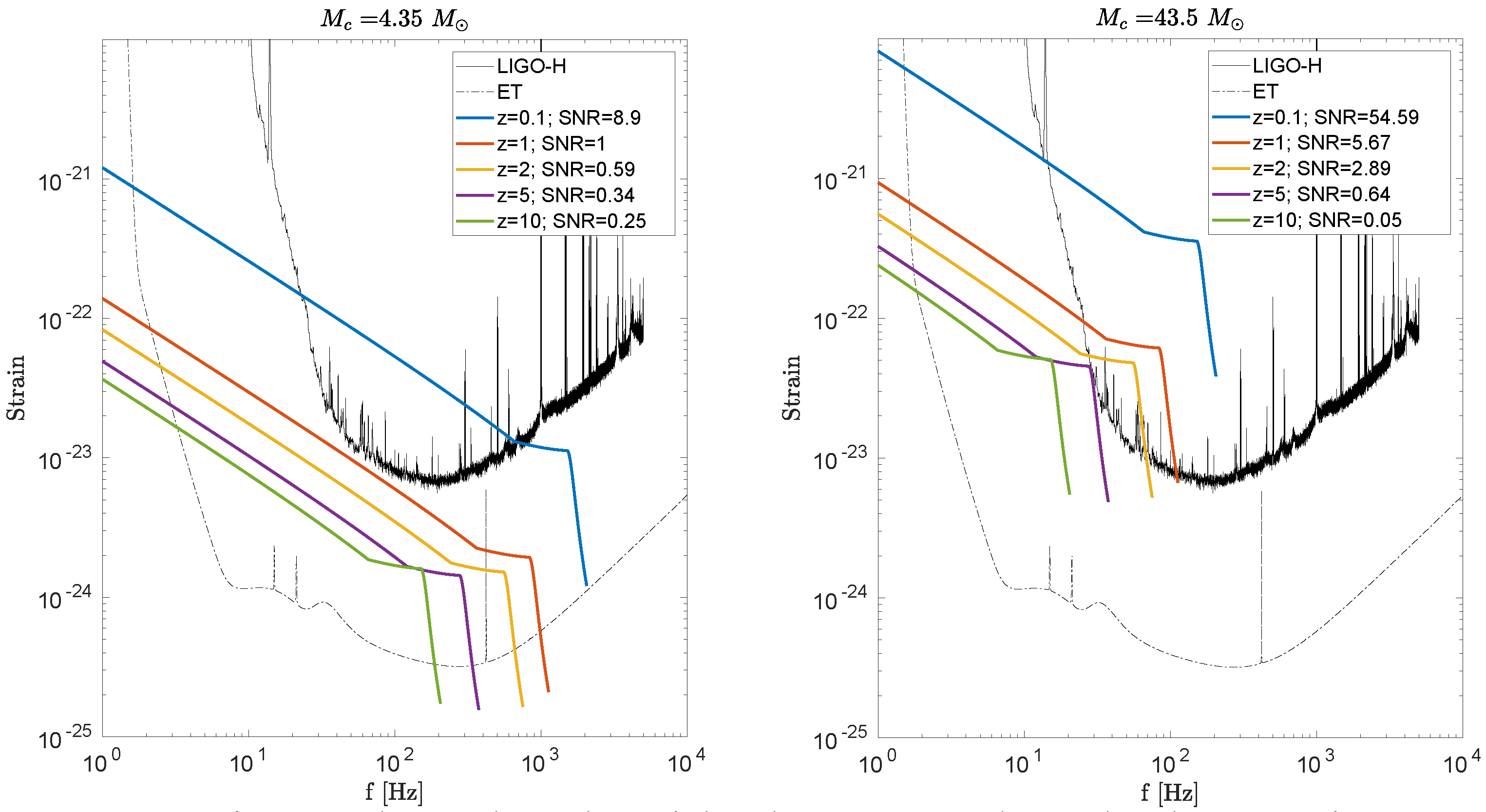
4.3. Compact Binary Population

We focused below on BBH events and assumed that their masses are in the range of [ 5 , 50 ] M [8,50]. We further assume that their formation rate is proportional to the cosmic star formation rate (SFR), for which we use the following parametric form [65]:
Ψ ( t ( z ) ) = A a e b ( z z m ) a b + b · e a ( z z m ) ,
with A = 0.24 M /yr/Mpc 3 , z m = 2.3 , a = 2.2 and b = 1.4 which peaks at z m . Note that we use this parameterization in the redshift range [ 0 , 20 ] even though it was derived using observations up to z = 9 . We define an efficiency parameter ϵ to describe the fraction of mass in BBH that merges within the age of the Universe that form out of a given stellar population. Moreover, we assume a delay time t delay between the formation of the progenitor star and the coalescence of the BBH, where the latter is distributed as
P d ( t delay ) t delay 1 ,
in the range [ t min , t max ] with t min = 50 Myr and t max equal to the age of the Universe. We also assume that the mass of the primary BH is distributed as
P ( m 1 ) m 1 α ,
in the range [ 5 , 50 ] M with α = 2.35 , while the mass of the secondary BH is uniformly distributed in the range [ 5 , m 1 ] so that p ( m 2 ) = c o n s t . in this range and p ( m 1 , m 2 ) = p ( m 1 ) p ( m 2 ) [50]. Note that this mass distribution is independent of redshift. We assume zero spins for all BHs. The merger rate is then given by the following integral over the delay time distribution:
d R d m 1 d m 2 d z = = ϵ T obs Ψ ( t ( z ) t delay ) p ( m 1 , m 2 ) P d ( t delay ) d V d z d t delay .
We calculate the SNR of each merger using Equation (12). We use the PhenomB inspiral–merger–ringdown waveforms to calculate the strain [66] and we use the noise power spectral density publicly available from [67,68]. We consider the event observable if it has ρ ρ lim = 10 . The normalization parameter ϵ was obtained by comparing the number of observable events in our model to the number of events observed during the first two LIGO/Virgo observational runs O1 + O2; note that the most recent merger rate from the O3 LIGO/Virgo catalog is on the low end but consistent with the O1 + O2 rate:
N obs = ρ ( m 1 , m 2 , z ) 10 d R d m 1 d m 2 d z d m 1 d m 2 d z
The merger rate per unit redshift and SNR is then calculated from Equation (27).
In Figure 4, we show the number of GW events per unit of SNR in different redshift bins. At low redshift, the slope and the width of the curves are constant; while at high redshift, the curves develop a low-SNR tail. The reason for this can be understood from Figure 5 where we plot the characteristic strain of BBH mergers with two different values of chirp mass (left and right panel) and for different redshifts, together with the O2 LIGO-Hanford detector noise (black solid) and the ET detector noise (black dashed). At low redshift, the SNR of high-mass events is always bigger than the one of low-mass events due to their higher amplitude. At high redshift, however, the sharp increase in the noise curve at low frequencies reduces the SNR of high masses more than the one of low masses which have higher frequencies so that the situation becomes actually reversed and low masses have a higher SNR. This leads to a spread of the SNR for different events over a large range. Of course, for all masses at high redshift, the SNR is very small and they can only be observed if they are highly magnified:

4.4. Probability of Strong Lensing for LIGO/Virgo Events

In Figure 6, we present the number density of magnified objects that we observe from a distance D obs as a function of magnification. We plot this quantity for three different values of D obs . In the right-hand panel of Figure 6, we multiply each line of the left-hand panel by the probability density of lensing as a function of magnification to obtain the (normalized) probability distribution of magnification for objects observed from different distances, D obs , i.e., Equation (21), as a function of magnification. Note that, while the number of objects which can be seen by the given survey (with fixed magnification) is somewhat lower for D obs = 3000 Mpc than for D obs = 500 Mpc, the probability of seeing such objects is higher for D obs = 3000 Mpc than for D obs = 500 Mpc. This is due to the fact that p ( μ , D obs ) is monotonically increases with D obs , as can be seen in Figure 3. For the product of p ( μ , D obs ) d N / d D obs , the increase in p wins over the decrease in N for D obs = 3000 Mpc.
In Figure 7, we plot the same quantities for different values of the cosmological redshift of the source. At a low redshift, d N / d z tends towards a constant at high magnification since we see all events (black curve, left panel). The product p ( z , μ ) d N / d z nearly tends towards a constant at high redshift which indicates that d N / d z grows similarly to μ 3 at high redshift (blue dashed curve, right panel).
In Figure 8, we present the results for the average amplification factor as a function of the cosmological redshift and luminosity distance of the sources (left panel) and as a function of observed redshift and luminosity distance of the sources (right panel). No sources are observable beyond 5500 Mpc. (This can be understood by computing the probability of seeing a source from a given observed distance, i.e., integrating p ( μ , D obs ) over μ . The probability of seeing an object from a distance bigger than 5000 Mpc is smaller than 10 7 .) The minimum amplification needed to detect sources from a redshift z s and with a given ρ max ( z s ) > ρ lim is given by
μ min ( z s ) = ρ lim ρ max 2 ,
hence, we can see sources from a maximum observed distance given by
D obs max ( z s ) = D ( z s ) μ min = D ( z s ) ρ max ( z s ) ρ lim .
For low redshifts, z s 2 , and we can work out the scaling of this quantity with redshift using a simple analytical approach, as can be seen in Appendix C. The probability P obs ( > μ ) that an object that LIGO/Virgo observes from a distance D obs was magnified more than μ is presented in Figure 9 for different values of D obs as a function of μ .

5. Discussion and Conclusions

Due to cosmological expansion, the frequencies of gravitational waves are redshifted. Since the frequencies of the GW signal from BBH mergers are degenerate with the mass, the quantity that we directly measure from the signal is the redshifted chirp mass M z = ( 1 + z ) M , where M is the intrinsic (true) chirp mass of the binary at a redshift z. The estimated luminosity distance can be converted into a redshift estimate (by choosing a cosmological model), which can, in turn, be used to estimate the intrinsic chirp mass M of the binary. The unknown lensing magnification will bias our estimation of the intrinsic mass and the distance (or equivalently, the redshift) of the binary. Therefore, lensed binaries will appear as a population at a lower redshift and with higher masses. The question is whether this effect is relevant for a given population of GW sources or whether it can be neglected.
In this article, we proposed a semi-analytical approach to study the lensing of gravitational waves by galaxies. The framework we propose can be applied to any detector or detector network once the strain noise of the observatory is known. We presented results for the probability of strong lensing for BBH visible by LIGO/Virgo, as a function of the redshift and magnification and for the average amplification as a function of cosmological redshift and observed distances. The numerical results are in good qualitative agreement with a simple model (valid for low redshift sources) that we present in a series of appendices.
Results for the probability that a source with cosmological redshift z s is magnified by μ are presented in Figure 3 as a function of both the cosmological and observed redshift (or rather distance) of the source. We stress that this result does not depend on the properties of the distribution of sources, nor on the specifics of a given observatory. The probability is small, but it slowly decays as a function of magnification. More specifically, for large values of magnification, the probability as a function of cosmological redshift scales as p ( μ , z s ) μ 3 . This scaling is independent of the lens distribution model. The probability density, as a function of the observed distance, p ( μ , D obs ) p ( μ , z s ( μ D obs ) ) , has an even slower decay with magnification, as can be seen in the right panel of Figure 3. Indeed, for a fixed D obs and μ > 1 , p ( μ , D obs ) p ( μ , z s ( μ D obs ) ) takes contributions from a higher redshift than z s ( D obs ) and is therefore larger. The exact scaling of p ( μ , D obs ) with μ depends on the details of the lens distribution. For a realistic distribution with a co-moving number density of lenses which fits numerical simulations (Illustris), we find that p ( μ , D obs ) μ α . The value of α increases from 2 to 3 as the observed luminosity distance varies from ∼300 Mpc to 5000 Mpc where it saturates to the asymptotic value α = 3 .
Selection effects related to the sensitivity curve (and hence to the horizon) of a given detector network enter into the game when computing the probability that a source that we can observe with a given observatory has a given magnification. This probability distribution P obs ( μ ) is defined in Equations (16) and (21) as a function of the cosmological redshift of a source and as a function of the observed luminosity distance, respectively. We focused on the LIGO/Virgo network in our analysis. Plots of the distribution of magnification for different cosmological redshifts and observed luminosity distances are presented in Figure 6 and Figure 7 (right panels). The distribution highly peaks at μ = 1 for low observed distances but it has more and more power at higher magnification as we move towards higher redshift or observed distances. The integral of this distribution multiplied by μ gives the average magnification expected for a given observed distance and the given experiment. For the LIGO/Virgo observatory, this is shown in Figure 8.
The probability distribution of magnification P obs ( μ ) for a given observed distance scales as P obs ( μ ) μ α + 1 / 2 and its integral from μ to infinity behaves as P obs ( > μ ) μ α + 3 / 2 for large values of μ with α [ 2 , 3 ] . The probability P obs ( > μ ) is presented in Figure 9 for different values of D obs . From this scaling, it follows that the mean of the magnification at small observed distances, which have α 2.5 , diverges at large μ . This is due to the presence of rare but extremely highly magnified sources, i.e., sources aligned along the lens–observer direction for which the magnification μ , see Equation (6). It also follows that, for any fixed value of D obs , the variance of the distribution diverges as μ α + 7 / 2 . We stress that this is a general property of the probability distribution of magnification, which is independent from the details of the distribution of sources. Moreover, it also applies to the case of strongly lensed sources of electromagnetic radiation. Furthermore, in that case, the variance of the distribution of magnification (for different observed redshift) is divergent. Physically, the magnification tends to a finite value and as mentioned above, the presence of the divergence is due to the geometric optics approximation, which breaks down in the vicinity of caustics, where wave effects need to be taken into account. Nevertheless, this indicates that the distribution has a significant tail with large magnification. The fact that the mean of the magnification only diverges for small observed distances is due to the fact that highly magnified sources appear to have small distances, D obs = D s / μ . In Figure 8, we present the results for the average amplification as a function of the cosmological and observed redshift of a source. A cut-off in μ was introduced to compute the mean for sources at low distances D obs < 1000 Mpc. We checked that our cut-off choice is such that increasing its value does not significantly affect the result. The average magnification, as a function of the observed redshift, is very close to 1 for a low redshift and it starts growing from z obs = 0.5 , reaching the maximum value of 40 at a redshift 0.8 where we stop seeing sources, i.e., where the horizon of the observatory (computed to allow for the presence of magnification) lies.
In a series of appendices, we present a semi-analytic model which allows us to study the impact of changing the underlying astrophysical model for both BBH and lens distribution on the resulting magnification distribution. Using this model, we verified that the average magnification (mildly) depends on the details of the source population, but that the qualitative picture of Figure 8 is expected to be valid—independently from the details of the chosen astrophysical model.
Let us finally derive some consequences for the LIGO/Virgo O1, O2 and O3 observations. The 74 published observed BBH (or binary black hole-Neutron star) events have distances of D obs [ 300 , 5300 ] Mpc. Assuming that the sensitivity has not significantly changed between O2 and O3, from the right panel of Figure 9, it follows that (for our modeling) the probability that one of them was magnified with a magnification of 10 or bigger is P obs ( > 10 ) 0.5 . (In Figure 9, the steep drop of the curves to the flatter slope happens between 1 < μ < 1.01 .) However, the probability that the magnification of one of them is bigger than 100 is not much smaller, namely P obs ( > 100 ) 0.03 . In order to infer that most or at least several of the observed events originated from cosmological redshifts z s 1–2, these would have to be magnified by a factor of approximately 100. While this is not improbable, for one of the events to be substantially magnified, it would require very significant changes in the lens population, which are in contradiction with both the observations and numerical simulations, indicating that this cannot be the case for several events, details of which can be found in Appendix B. Another possibility would be a very significant change in the source distribution which would have to be approximately 1000 times larger at z s 1–2 and correspondingly smaller at z 0 . This, however, is at very strong odds with stellar evolution models. We therefore conclude that even though the lensing of GW observations will be relevant in the future, e.g., for the analysis of standard sirens, we cannot reasonably ’tweak’ galaxy population models or stellar evolution models so that we can conclude that most of the observed LIGO/Virgo detections are strongly lensed, as proposed in [16,17,27,36].
The framework used in this analysis is flexible and can be adapted to study the strong and weak lensing of sources in any frequency band, and it can be applied to any detector network. In this work, we have focused on the case of the LIGO/Virgo network. We stress that while for the case of LIGO/Virgo, the contribution of weak lensing is negligible, this is not the case for instruments with a sensitivity such that the peak of the redshift distribution of sources is typically within the instrument horizon. In this case, the weak lensing contribution to the distribution of μ has to be added using, e.g., the results of ray tracing simulations. Then, a p ( μ , z ) which describes both weak and strong lensing can be used to derive the corresponding distribution of P ( μ ) and P obs ( μ ) (including selection effects) following the procedure illustrated in this work, as can be seen in, e.g., [70], for a recent analysis of the weak and strong lensing of massive black hole binaries visible by LISA.

Author Contributions

Conceptualization, R.D. and G.C. All three authors contributed to the required theoretical calculations and to the writing of the paper. All authors have read and agreed to the published version of the manuscript.

Funding

This project has received funding from the European Research Council (ERC) under the European Union’s Horizon 2020 research and innovation program (grant agreement No. 693024) and from the Swiss National Science Foundation.

Institutional Review Board Statement

Not applicable.

Informed Consent Statement

Not applicable.

Acknowledgments

It is a pleasure to thank Michele Maggiore and Nicola Tamanini for helpful discussions. We also thank Paul Torrey for providing us with the analytic fitting formula of [59]. We are grateful also to XiKai Shan who pointed out a relevant error in the first version of this paper.

Conflicts of Interest

The funders had no role in the design of the study; in the collection, analyses, or interpretation of data; in the writing of the manuscript, or in the decision to publish the results.

Appendix A. Fit to the Illustris Simulation

The functions A, α , β and γ of the fitting formula used in Section 4.1 to describe the evolution of galaxy as a function of redshift and velocity dispersion [63] are modeled as
A = A 0 + A 1 z + A 2 z 2 ,
α = α 0 + α 1 z + α 2 z 2 ,
β = β 0 + β 1 z + β 2 z 2 ,
γ = γ 0 + γ 1 z + γ 2 z 2 .
In the following table, we list the values of the coefficients.
i i = 0 i = 1 i = 2
A i 7.3914985.729400−1.120552
α i −6.863393−5.2732711.104114
β i 2.8520831.255696−0.286638
γ i 0.067032−0.0486830.007648

Appendix B. Analytic Description of Lens Distribution

If there was no evolution of lenses, we would expect the physical number density of galaxies to scale with redshift as n ( σ v , z ) ( 1 + z ) 3 , hence:
0 d σ v σ v 4 n ( σ v , z ) = ( 1 + z ) 3 N σ v 4 ,
where N is the present galaxy density:
N = 0 d σ v n ( σ v , z = 0 ) ,
and σ v 4 is the mean of the velocity dispersion to power 4. Let us now assume that, in the considered redshift range, it is legitimate to neglect evolution, and hence the physical density scales with the expansion of the Universe. We postulate this law of evolution, not because it is very realistic, but because it allows us to analytically integrate the optical depth. However, as we shall see in the next section, for low redshifts to which present gravitational wave experiments are sensitive, this model is actually quite good.
Neglecting evolution, the factor 1 / ( 1 + z ) 3 in (9) cancels out and using χ ( z , z s ) = H ( z ) 1 , we obtain:
τ ( μ , z s ) = π ( 4 π ) 2 σ v 4 N χ s 2 1 ( μ 1 ) 2 0 χ s d χ ( χ s χ ) 2 χ 2 = π ( 4 π ) 2 σ v 4 N χ s 3 30 ( μ 1 ) 2 .
Crude estimates for N and σ v are (our value of σ v is one of large galaxies and N is obtained by simply dividing ρ m = Ω m ρ c by the mass of a large galaxy, M gal 10 12 M .)
N = 10 9 H 0 3 , σ v 4 = ( 150 km / s ) 4 5 × 10 14 .
As we set c = 1 , we have H 0 = h / ( 3000 Mpc ) . With this, we obtain:
τ ( μ , z s ) 0.001 ( μ 1 ) 2 ( H 0 χ ( z s ) ) 3 N 10 9 H 0 3 σ v 4 5 × 10 14 .
for the optical depth.
This analytic model gives a result for optical depth in good agreement with the one obtained in Section 4.2 considering a more realistic distribution of lenses, which evolves with redshift (fractional deviations of a few percent). For our simple model, we find for the probability density of magnification as a function of the cosmological source redshift:
p ( μ , z s ) = 2 p 1 ( z s ) ( μ 1 ) 3 exp p 1 ( z s ) ( μ 1 ) 2 , where
p 1 ( z s ) = 0.001 ( H 0 χ ( z s ) ) 3 N 10 9 H 0 3 σ v 4 5 × 10 14 .
Already from this expression, it is clear that we cannot achieve a significant probability of amplification at low redshifts. With this probability distribution, the mean magnification for a source from redshift z s is μ ( z s ) = 1 + π p 1 ( z s ) . To obtain a non-negligible probability for magnification by a factor of 50 or more, which is needed to explain the observed GW events as highly magnified events from redshift z s 1–2, we require that p 1 1000 . The factor H 0 χ ( z s ) in Equation (A11) becomes of order unity at redshift z s 1.5 and then very slowly grows up to H 0 χ ( z s ) 2 at z s 10 . This requires a galaxy density which is more than 10 6 times higher than 10 9 H 0 3 or σ v 4500 km/s or a combination of both such that:
N 10 9 H 0 3 σ v 4 ( 150 km / s ) 4 > 10 6 .
These possibilities are very strongly ruled out by present astronomical observations and by numerical simulations, as can be seen, e.g., in Section 4.
To have some intuition regarding the role of the redshift evolution of the galaxy velocity dispersion function, we compare the results obtained in Section 4 using the Illustris simulation to a non-evolving lens distribution. For this, we use the distribution function (22) for z = 0 , assuming no redshift evolution. We then have:
n no evo ( σ v , z ) = ( 1 + z ) 3 n com ( σ v , z = 0 ) .
The comparison is shown in Figure A1. The result is valid for arbitrary magnification μ .
Figure A1. Relative difference between the probability with and without redshift evolution. The result is valid for arbitrary magnification μ .
Universe 08 00019 g0a1
At low redshift, 0 < z < 2 , the non-evolving distribution actually has somewhat less galaxies with low-velocity dispersion, which are the most numerous ones, and therefore the evolving distribution leads to a higher probability for magnification than the non-evolving one, δ P > 0 . At higher redshift z > 4 , the loss of lenses in the evolving distribution becomes more relevant and δ P changes sign. However, the difference between the evolving and non-evolving distribution is never larger than 10% for redshift z 6 . This tells us that our results are quite insensitive to the redshift evolution of the lenses.

Appendix C. Analytical Description of BBH Population

In this appendix, we work out an analytic model to describe the number density of sources as a function of the emitted gravitational-wave strain amplitude (or the SNR for a given detector configuration) and as a function of redshift. As a first step, we review the derivation of the SNR of a binary system of compact objects at fixed redshift as a function of the component masses and of the noise power spectral density of the instrument(s). We introduce the SNR per unit frequency ρ for a binary that merges at redshift z s and is observed in a narrow frequency band around f as [57]
ρ 2 ( f , z s ) = 4 | h ( f , z s ) | 2 S n ( f ) F ( f , z s ) S n ( f ) ,
where S n ( f ) is the noise power spectrum of a given detector network, with a dimension of Hz 1 and h ( f , z s ) is the Fourier transform of the strain, with dimensions Hz 1 . The total SNR in the frequency band of a given detector is simply the integral of Equation (A14) over that band. In Equation (A14), we defined the received flux per unit of frequency as F ( f , z s ) . Hence, there is a one-to-one mapping between flux and SNR. For a single binary system, the SNR from the inspiral phase integrated over observed frequency is given by [57] (neglecting the merger and ringdown phases and writing the quantities upon which the SNR explicitly depends:)
ρ 2 ( z s , m , M ) = 5 96 π 4 / 3 Θ 2 D 2 ( z s ) ( G M z ) 5 / 3 f 7 / 3 ( z s , m ) ,
where M z = M ( 1 + z s ) is the redshifted chirp mass of the system, m = m 1 + m 2 is the total mass and the integral over frequencies can be approximated by
f 7 / 3 ( z s , m ) 0 f ISCO / ( 1 + z s ) d f f 7 / 3 S n ( f ) 1 ,
with dimension [ f 7 / 3 ] = [ Hz ] 1 / 3 , while Θ 2 (with 0 Θ 2 16 ) is a geometrical factor that depends on the inclination of the binary and on the antenna pattern of the detector. Averaging over all angles, one finds that Θ 2 ¯ = 64 / 25 . We do not need this explicit expression in what follows and the interested reader is referred to [57] for details. In Equation (A16), the upper integration bound is given by the (redshifted) frequency corresponding to the innermost stable circular orbit (ISCO) of the system, i.e., the frequency at which we consider the inspiraling phase of the system to end in our approximation. It is defined as [58]
f ISCO 1 6 6 ( 2 π ) c 3 G m 2.2 kHz M m ,
where m is again the total mass of the binary system. This frequency is not the frequency where the signal is maximal, but it is the frequency beyond which we can no longer trust the quadrupole formula used for the SNR estimate in Equation (A15). It is therefore a conservative estimate of the SNR which has contributions from higher frequencies, e.g., the coalescence frequency is typically approximately 3 f ISCO . However, we follow here the standard procedure as detailed in [57]. We rewrite the parameterization (A15) in a way which will be useful for what follows:
ρ 2 ( z s , M , m ) = = 7.7 · 10 39 Θ 2 M M 5 / 3 Mpc D ( z s ) 2 f 7 / 3 ( z s , m ) Hz 1 / 3 ( 1 + z s ) 5 / 3 .
Let us understand the redshift dependence: from Equation (A16), we see that if f ISCO / ( 1 + z s ) > f max , then f 7 / 3 ( z s ) does not depend on redshift. Here, with f max , we denote the maximum frequency a given detector is sensitive to (i.e., the frequency above which the noise becomes very large) and it is fixed by the form of the spectral noise in Equation (A16). This is determined by the condition:
( 1 + z s ) < f ISCO f max 2.2 . kHz f max M m .
If this condition is verified for a given source, then (A16) is redshift independent.
From a comparison with numerical models for source formation and evolution (see Section 4), we find that the maximum SNR that we receive from a given redshift z s can be effectively written as
ρ max ( z s ) = A M max M 5 / 6 Mpc D ( z s ) ( 1 + z s ) 5 / 6 f ¯ 7 / 3 ( z s ) 1 / 2 ,
and similarly for the minimum value:
ρ min ( z s ) = A M min M 5 / 6 Mpc D ( z s ) ( 1 + z s ) 5 / 6 f ¯ 7 / 3 ( z s ) 1 / 2 ,
where f ¯ 7 / 3 ( z s ) 1 / 2 is obtained using the average ISCO frequency in Hz, rescaled with redshift, as the upper cutoff in the integral (A16), i.e., the ISCO frequency for the average total mass m. We introduced a constant A = 1.4 × 10 19 which corresponds to the square root of the numerical factor in Equation (A18) multiplied by the square root of Θ ¯ 2 = 64 / 25 . We denoted by M min and M max the minimum and maximum value of the chirp mass (for a given mass distribution), respectively. We observed that for redshifts that satisfy the condition (A19), Equations (A20) and (A21) simply scale with redshift as ( 1 + z s ) 5 / 6 D ( z s ) 1 .
As a second step, we need a parameterization for the number of sources per unit of SNR as a function of SNR and of redshift. The number density of sources per unit of chirp mass (and as a function of redshift) is given by
N ( z s , M c ) R ( z s , M c ) p ( M c ) ,
where R is the merger rate for a binary system with chirp mass M c at redshift z s , which in turn is proportional to the distribution of chirp masses (with a redshift-dependent pre-factor). For simplicity, we assume it to be monomial, p ( M c ) M c β M . We now convert the number density (A22) into a number density per unit of SNR. Neglecting the mass dependence of the ISCO frequency, as we did in (A20) and (A21), we can simply invert (A18) and we obtain for the distribution of sources as a function of SNR:
N ( ρ , z s ) = N ρ ( z s ) ρ γ for   ρ min ( z s ) < ρ < ρ max ( z s ) , 0 otherwise ,
with γ = ( 6 β M 1 ) / 5 and N ρ ( z s ) which is a redshift-dependent function. For example, the distribution of masses in the astrophysical model discussed in Section 4 is such that the resulting distribution of chirp masses is (independent on redshift) p ( M c ) M c 3.2 . Then, N ( ρ , z s ) ρ 3.6 , which is the scaling of the curves in Figure A2. Note that when comparing this figure to the scaling derived here, one needs to keep in mind that d N / d ρ = ρ 1 d N / d log ρ .
Figure A2. Comparison between the analytic model for source distribution presented in Appendix C and the numerical simulations of Section 4.3, for different redshifts 0.0125 z 2.5075 . The dashed line represents the scaling given in Equation (A23) with γ = 3.6 .
Universe 08 00019 g0a2

Appendix D. Analytic Derivation of the Average Magnification

The number of sources which we see from redshift z s with our limiting SNR ρ lim , if magnified by μ , is:
N ( ρ lim , z s , μ ) = N ρ ( z s ) α lim ρ 2 ( z s ) d ρ ρ γ = N ρ ( z s ) γ 1 1 α lim γ 1 1 ρ 2 ( z s ) γ 1 ,
where α lim = max ρ lim / μ , ρ 1 ( z s ) and we set ρ 1 ρ min , ρ 2 ρ max . We assume that ρ lim / μ < ρ 2 ( z s ) . If this is not the case, then N ( ρ lim , z s , μ ) = 0 . We assume here that γ 1 but the case γ = 1 can be easily worked out following steps similar to the ones performed below. The result without magnification is simply N ( ρ lim , z s , 1 ) . The total number of sources which we see is therefore:
N ( ρ lim , z s ) = 1 d μ p ( μ , z s ) N ( ρ lim , z s , μ ) .
With a bit of algebra, this can be rewritten as
N ( ρ lim , z s ) = N ρ γ 1 ( ρ 1 γ + 1 ρ 2 γ + 1 ) + N ρ γ 1 [ ρ 2 γ + 1 1 ( ρ lim / ρ 2 ) 2 d μ p ( μ , z s ) ρ 1 γ + 1 1 ( ρ lim / ρ 1 ) 2 d μ p ( μ , z s ) + ( ρ lim / ρ 2 ) 2 ( ρ lim / ρ 1 ) 2 d μ p ( μ , z s ) μ ρ lim γ 1 ] ,
where the redshift dependence in ρ 1 , 2 and N ρ is understood. We eventually want to compute the average magnification. For this, we need to compute:
M ( ρ lim , z s ) 1 d μ μ p ( μ , z s ) N ( ρ lim , z s , μ ) ,
which can be done with similar steps as above, yielding:
M ( ρ lim , z s ) = N ρ γ 1 ( ρ 1 γ + 1 ρ 2 γ + 1 ) μ ¯ + N ρ γ 1 [ ρ 2 γ + 1 1 ( ρ lim / ρ 2 ) 2 d μ μ p ( μ , z s ρ 1 γ + 1 1 ( ρ lim / ρ 1 ) 2 d μ μ p ( μ , z s ) + ( ρ lim / ρ 2 ) 2 ( ρ lim / ρ 1 ) 2 d μ μ p ( μ , z s ) μ ρ lim γ 1 ] ,
where μ ¯ depends on the source redshift and is defined as
μ ¯ ( z s ) = 1 d μ μ p ( μ , z s ) .
The average magnification is now given by the ratio of (A28) over (A24):
μ ( z s ) = M ( ρ lim , z s ) / N ( ρ lim , z s ) .
The computation of the average magnification presented in this section relies on the assumption that we can replace the mass dependence of the ISCO frequency appearing in the expression of the SNR (A18) by an average. From a comparison with the numerical models of Section 4, it turns out that this approximation is well justified for low redshift sources ( z s < 2 when considering the sensitivity curve of the LIGO/Virgo detectors). The comparison is shown in Figure A2. As already explained, the average magnification does not depend on the scaling of the number of events with redshift, i.e., on N ρ ( z s ) in Equation (A23). To compare with a realistic population model, in Figure A2, we reconstructed this dependence fitting the numerical model, i.e., N ρ ( z s ) ρ 3 . For high redshift sources, a simple analytic derivation of the average magnification is not possible, but the relation (A18) can be numerically inverted to find the chirp mass and the average magnification can be numerically computed as a function of redshift.

Appendix E. Analytical Results for the LIGO Detector(s)

Our analytic model for the distribution of sources has four free parameters: ( γ , M min , M max ) defining the distribution of chirp masses and ρ lim (or equivalently S n ) which gives the minimum SNR for detection, and depends on the detector network chosen. We focus now on the case of the LIGO detectors and we compute the average magnification for different choices of the parameters ( γ , M min , M max ). For definiteness, we consider the noise curve of the LIGO-Livingstone detector for the O2 run. The sensitivity for O3 is slightly better. In Figure A3, we plot the spectral noise of the LIGO-Livingstone detector that we find to be well described by the fitting function S fit ( f ) given by
S fit ( f ) = A s f 30 Hz α s + 1 exp β s log f 150 Hz 2 ,
with log 10 A s = 46.3 , α s = 7.8 and β s = 0.4 .
Figure A3. Spectral noise curve for the LIGO-Livingstone detector [71]. The red curve is the fit given in Equation (A31).
Universe 08 00019 g0a3
We analyze the dependence of the average amplification on the details of the astrophysical model. In particular, we want to explore the dependence on the distribution of the component masses and on the upper cut-off in the distribution. We assume that the primary BH mass is distributed as p ( m 1 ) m 1 α in the range [ 5 , X ] M where both α and X are parameters that we vary. We consider two cases: α = 2.35 and α = 1.5 . The corresponding normalized distribution of chirp masses is polynomial in the chirp mass, i.e., p ( M c ) M c β M with β M = 3.2 and β M = 2.1 , respectively. As explained in the previous section, for a sufficiently small redshift, the scaling of the number density of sources per unit of signal to noise is given by (A23) with γ = 1 / 5 ( 1 6 β M ) ; hence, γ = 3.6 and 2.3 for the two values of α , respectively. In Figure A4, we show results for the average magnification as a function of redshift for the two models considered and for two different values of the upper cut-off in the mass distribution. The result for the average amplification in Figure A4 is in excellent agreement with the one we found using a realistic model for source formation and evolution for low redshift sources (as can be seen in Figure 8, left panel).
Figure A4. (Left) Average magnification for α = 2.35 ( γ = 3.6 ) for two different upper cut-offs in the distribution of the primary mass. (Right) Average magnification for α = 1.5 ( γ = 2.3 ) for two different upper cut-offs in the distribution of the primary mass.
Universe 08 00019 g0a4

References

  1. Abbott, B.P. et al. [LIGO Scientific Collaboration and Virgo Collaboration] Observation of Gravitational Waves from a Binary Black Hole Merger. Phys. Rev. Lett. 2016, 116, 061102. [Google Scholar] [CrossRef]
  2. Abbott, B.P. et al. [LIGO Scientific Collaboration and Virgo Collaboration] GW151226: Observation of Gravitational Waves from a 22-Solar-Mass Binary Black Hole Coalescence. Phys. Rev. Lett. 2016, 116, 241103. [Google Scholar] [CrossRef]
  3. Abbott, B.P. et al. [LIGO Scientific Collaboration and Virgo Collaboration] Binary Black Hole Mergers in the first Advanced LIGO Observing Run. Phys. Rev. 2016, X6, 041015. [Google Scholar] [CrossRef]
  4. Abbott, B.P. t al. [LIGO Scientific Collaboration and Virgo Collaboration]. GW170608: Observation of a 19-solar-mass Binary Black Hole Coalescence. Astrophys. J. 2017, 851, L35. [Google Scholar] [CrossRef]
  5. Abbott, B.P. et al. [LIGO Scientific Collaboration and Virgo Collaboration] GW170814: A Three-Detector Observation of Gravitational Waves from a Binary Black Hole Coalescence. Phys. Rev. Lett. 2017, 119, 141101. [Google Scholar] [CrossRef] [PubMed] [Green Version]
  6. Abbott, B.P. et al. [LIGO Scientific and Virgo Collaboration] GW170104: Observation of a 50-Solar-Mass Binary Black Hole Coalescence at Redshift 0.2. Phys. Rev. Lett. 2017, 118, 221101. [Google Scholar] [CrossRef] [PubMed] [Green Version]
  7. Abbott, B.P. et al. [LIGO Scientific Collaboration and Virgo Collaboration] GW170817: Observation of Gravitational Waves from a Binary Neutron Star Inspiral. Phys. Rev. Lett. 2017, 119, 161101. [Google Scholar] [CrossRef] [PubMed] [Green Version]
  8. Abbott, B.P. et al. [LIGO Scientific Collaboration and Virgo Collaboration] GWTC-1: A Gravitational-Wave Transient Catalog of Compact Binary Mergers Observed by LIGO and Virgo during the First and Second Observing Runs. Phys. Rev. 2019, X9, 031040. [Google Scholar] [CrossRef] [Green Version]
  9. Abbott, R. et al. [LIGO Scientific Collaboration and Virgo Collaboration] GWTC-2: Compact Binary Coalescences Observed by LIGO and Virgo during the First Half of the Third Observing Run. Phys. Rev. X 2021, 11, 021053. [Google Scholar] [CrossRef]
  10. Abbott, R. et al. [LIGO Scientific Collaboration, Virgo Collaboration, and KAGRA Collaboration] Observation of Gravitational Waves from Two Neutron Star–Black Hole Coalescences. Astrophys. J. Lett. 2021, 915, L5. [Google Scholar] [CrossRef]
  11. Abbott, R. et al. [LIGO Scientific Collaboration, Virgo Collaboration, and KAGRA Collaboration] GWTC-3: Compact Binary Coalescences Observed by LIGO and Virgo During the Second Part of the Third Observing Run. arXiv 2021, arXiv:2111.03606. [Google Scholar]
  12. Oguri, M. Effect of gravitational lensing on the distribution of gravitational waves from distant binary black hole mergers. Mon. Not. R. Astron. Soc. 2018, 480, 3842–3855. [Google Scholar] [CrossRef] [Green Version]
  13. Wang, Y.; Stebbins, A.; Turner, E.L. Gravitational Lensing of Gravitational Waves from Merging Neutron Star Binaries. Phys. Rev. Lett. 1996, 77, 2875–2878. [Google Scholar] [CrossRef]
  14. Sereno, M.; Sesana, A.; Bleuler, A.; Jetzer, P.; Volonteri, M.; Begelman, M.C. Strong Lensing of Gravitational Waves as Seen by LISA. Phys. Rev. Lett. 2010, 105, 251101. [Google Scholar] [CrossRef] [PubMed] [Green Version]
  15. Ng, K.K.Y.; Wong, K.W.K.; Broadhurst, T.; Li, T.G.F. Precise LIGO Lensing Rate Predictions for Binary Black Holes. Phys. Rev. 2018, D97, 023012. [Google Scholar] [CrossRef] [Green Version]
  16. Broadhurst, T.; Diego, J.M.; Smoot, G. Reinterpreting Low Frequency LIGO/Virgo Events as Magnified Stellar-Mass Black Holes at Cosmological Distances. arXiv 2018, arXiv:1802.05273. [Google Scholar]
  17. Broadhurst, T.; Diego, J.M.; Smoot, G.F. Twin LIGO/Virgo Detections of a Viable Gravitationally-Lensed Black Hole Merger. arXiv 2019, arXiv:1901.03190. [Google Scholar]
  18. Haris, K.; Mehta, A.K.; Kumar, S.; Venumadhav, T.; Ajith, P. Identifying strongly lensed gravitational wave signals from binary black hole mergers. arXiv 2018, arXiv:1807.07062. [Google Scholar]
  19. Cao, Z.; Li, L.F.; Wang, Y. Gravitational lensing effects on parameter estimation in gravitational wave detection with advanced detectors. Phys. Rev. D 2014, 90, 062003. [Google Scholar] [CrossRef] [Green Version]
  20. Dai, L.; Venumadhav, T. On the waveforms of gravitationally lensed gravitational waves. arXiv 2017, arXiv:1702.04724. [Google Scholar]
  21. Dai, L.; Li, S.S.; Zackay, B.; Mao, S.; Lu, Y. Detecting Lensing-Induced Diffraction in Astrophysical Gravitational Waves. Phys. Rev. D 2018, 98, 104029. [Google Scholar] [CrossRef] [Green Version]
  22. Dai, L.; Venumadhav, T.; Sigurdson, K. Effect of lensing magnification on the apparent distribution of black hole mergers. Phys. Rev. D 2017, 95, 044011. [Google Scholar] [CrossRef] [Green Version]
  23. Jung, S.; Shin, C.S. Gravitational-Wave Fringes at LIGO: Detecting Compact Dark Matter by Gravitational Lensing. Phys. Rev. Lett. 2019, 122, 041103. [Google Scholar] [CrossRef] [PubMed] [Green Version]
  24. Lai, K.H.; Hannuksela, O.A.; Herrera-Martín, A.; Diego, J.M.; Broadhurst, T.; Li, T.G.F. Discovering intermediate-mass black hole lenses through gravitational wave lensing. Phys. Rev. D 2018, 98, 083005. [Google Scholar] [CrossRef] [Green Version]
  25. Smith, G.P.; Jauzac, M.; Veitch, J.; Farr, W.M.; Massey, R.; Richard, J. What if LIGO’s gravitational wave detections are strongly lensed by massive galaxy clusters? Mon. Not. R. Astron. Soc. 2018, 475, 3823–3828. [Google Scholar] [CrossRef]
  26. Shan, X.; Wei, C.; Hu, B. Lensing magnification: Gravitational waves from coalescing stellar-mass binary black holes. arXiv 2020, arXiv:2012.08381. [Google Scholar] [CrossRef]
  27. Diego, J.M.; Broadhurst, T.; Smoot, G. Evidence for lensing of gravitational waves from LIGO-Virgo. arXiv 2021, arXiv:2106.06545. [Google Scholar] [CrossRef]
  28. Pagano, G.; Hannuksela, O.A.; Li, T.G.F. lensingGW: A Python package for lensing of gravitational waves. Astron. Astrophys. 2020, 643, A167. [Google Scholar] [CrossRef]
  29. Mukherjee, S.; Wandelt, B.D.; Silk, J. Probing the theory of gravity with gravitational lensing of gravitational waves and galaxy surveys. Mon. Not. R. Astron. Soc. 2020, 494, 1956–1970. [Google Scholar] [CrossRef]
  30. Chung, K.W.; Li, T.G.F. Lensing of Gravitational Waves as a Novel Probe of Graviton Mass. arXiv 2021, arXiv:2106.09630. [Google Scholar] [CrossRef]
  31. Urrutia, J.; Vaskonen, V. Lensing of gravitational waves as a probe of compact dark matter. arXiv 2021, arXiv:2109.03213. [Google Scholar] [CrossRef]
  32. Cremonese, P.; Mota, D.F.; Salzano, V. Characteristic features of gravitational wave lensing as probe of lens mass model. arXiv 2021, arXiv:2111.01163. [Google Scholar]
  33. Hannuksela, O.A.; Haris, K.; Ng, K.K.Y.; Kumar, S.; Mehta, A.K.; Keitel, D.; Li, T.G.F.; Ajith, P. Search for gravitational lensing signatures in LIGO-Virgo binary black hole events. Astrophys. J. 2019, 874, L2. [Google Scholar] [CrossRef] [Green Version]
  34. Oguri, M. Strong gravitational lensing of explosive transients. Rept. Prog. Phys. 2019, 82, 126901. [Google Scholar] [CrossRef] [PubMed] [Green Version]
  35. Diego, J.M. Constraining the abundance of primordial black holes with gravitational lensing of gravitational waves at LIGO frequencies. arXiv 2019, arXiv:1911.05736. [Google Scholar] [CrossRef]
  36. Broadhurst, T.; Diego, J.M.; Smoot, G.F. Interpreting LIGO/Virgo “Mass-Gap” events as lensed Neutron Star-Black Hole binaries. arXiv 2020, arXiv:2006.13219. [Google Scholar]
  37. Gavazzi, R.; Treu, T.; Rhodes, J.D.; Koopmans, L.V.; Bolton, A.S.; Burles, S.; Massey, R.; Moustakas, L.A. The Sloan Lens ACS Survey. 4. The mass density profile of early-type galaxies out to 100 effective radii. Astrophys. J. 2007, 667, 176–190. [Google Scholar] [CrossRef]
  38. Robertson, A.; Smith, G.P.; Massey, R.; Eke, V.; Jauzac, M.; Bianconi, M.; Ryczanowski, D. What does strong gravitational lensing? The mass and redshift distribution of high-magnification lenses. arXiv 2020, arXiv:2002.01479. [Google Scholar] [CrossRef]
  39. Belczynski, K.; Holz, D.E.; Bulik, T.; O’Shaughnessy, R. The first gravitational-wave source from the isolated evolution of two 40–100 Msun stars. Nature 2016, 534, 512. [Google Scholar] [CrossRef] [Green Version]
  40. Eldridge, J.J.; Stanway, E.R. BPASS predictions for Binary Black-Hole Mergers. Mon. Not. R. Astron. Soc. 2016, 462, 3302–3313. [Google Scholar] [CrossRef] [Green Version]
  41. Wysocki, D.; Gerosa, D.; O’Shaughnessy, R.; Belczynski, K.; Gladysz, W.; Berti, E.; Kesden, M.; Holz, D.E. Explaining LIGO’s observations via isolated binary evolution with natal kicks. Phys. Rev. D 2018, 97, 043014. [Google Scholar] [CrossRef] [Green Version]
  42. Dvorkin, I.; Uzan, J.P.; Vangioni, E.; Silk, J. Exploring stellar evolution with gravitational-wave observations. Mon. Not. R. Astron. Soc. 2018, 479, 121–129. [Google Scholar] [CrossRef] [Green Version]
  43. Kruckow, M.U.; Tauris, T.M.; Langer, N.; Kramer, M.; Izzard, R.G. Progenitors of gravitational wave mergers: Binary evolution with the stellar grid-based code ComBinE. Mon. Not. R. Astron. Soc. 2018, 481, 1908–1949. [Google Scholar] [CrossRef]
  44. Spera, M.; Mapelli, M.; Giacobbo, N.; Trani, A.A.; Bressan, A.; Costa, G. Merging black hole binaries with the SEVN code. Mon. Not. R. Astron. Soc. 2019, 485, 889–907. [Google Scholar] [CrossRef] [Green Version]
  45. Mapelli, M.; Giacobbo, N.; Santoliquido, F.; Artale, M.C. The properties of merging black holes and neutron stars across cosmic time. Mon. Not. R. Astron. Soc. 2019, 487, 2–13. [Google Scholar] [CrossRef]
  46. Rodriguez, C.L.; Zevin, M.; Amaro-Seoane, P.; Chatterjee, S.; Kremer, K.; Rasio, F.A.; Ye, C.S. Black holes: The next generation—Repeated mergers in dense star clusters and their gravitational-wave properties. Phys. Rev. D 2019, 100, 043027. [Google Scholar] [CrossRef] [Green Version]
  47. Stevenson, S.; Sampson, M.; Powell, J.; Vigna-Gómez, A.; Neijssel, C.J.; Szécsi, D.; Mandel, I. The impact of pair-instability mass loss on the binary black hole mass distribution. Astrophys. J. 2019, 882, 121. [Google Scholar] [CrossRef]
  48. Fragione, G.; Leigh, N.; Perna, R. Black hole and neutron star mergers in Galactic Nuclei: The role of triples. Mon. Not. R. Astron. Soc. 2019, 488, 2825–2835. [Google Scholar] [CrossRef] [Green Version]
  49. Woosley, S.E.; Heger, A. The Pair-Instability Mass Gap for Black Holes. Astrophys. J. Lett. 2021, 912, L31. [Google Scholar] [CrossRef]
  50. Abbott, B.P. et al. [LIGO Scientific Collaboration and Virgo Collaboration] Binary Black Hole Population Properties Inferred from the First and Second Observing Runs of Advanced LIGO and Advanced Virgo. Astrophys. J. 2019, 882, L24. [Google Scholar] [CrossRef] [Green Version]
  51. Turner, E.L.; Ostriker, J.P.; Gott, J. Richard, I. The Statistics of gravitational lenses: The Distributions of image angular separations and lens redshifts. Astrophys. J. 1984, 284, 1–22. [Google Scholar] [CrossRef]
  52. Fukugita, M.; Futamase, T.; Kasai, M.; Turner, E.L. Statistical Properties of Gravitational Lenses with a Nonzero Cosmological Constant. Astrophys. J. 1992, 393, 3. [Google Scholar] [CrossRef]
  53. Oguri, M.; Marshall, P.J. Gravitationally lensed quasars and supernovae in future wide-field optical imaging surveys. Mon. Not. R. Astron. Soc. 2010, 405, 2579–2593. [Google Scholar] [CrossRef] [Green Version]
  54. Hilbert, S.; White, S.D.; Hartlap, J.; Schneider, P. Strong lensing optical depths in a LambdaCDM universe. Mon. Not. R. Astron. Soc. 2007, 382, 121–132. [Google Scholar] [CrossRef] [Green Version]
  55. Hilbert, S.; White, S.D.; Hartlap, J.; Schneider, P. Strong lensing optical depths in a LCDM Universe. 2. The influence of the stellar mass in galaxies. Mon. Not. R. Astron. Soc. 2008, 386, 1845–1854. [Google Scholar] [CrossRef] [Green Version]
  56. Schneider, P.; Ehlers, J.; Falco, E.E. Gravitational Lenses; Springer: Berlin/Heidelberg, Germany, 1992. [Google Scholar] [CrossRef]
  57. Finn, L.S.; Chernoff, D.F. Observing binary inspiral in gravitational radiation: One interferometer. Phys. Rev. 1993, D47, 2198–2219. [Google Scholar] [CrossRef] [Green Version]
  58. Maggiore, M. Gravitational Waves. Vol. 1: Theory and Experiments; Oxford Master Series in Physics; Oxford University Press: Oxford, UK, 2007. [Google Scholar]
  59. Torrey, P.; Wellons, S.; Machado, F.; Griffen, B.; Nelson, D.; Rodriguez-Gomez, V.; McKinnon, R.; Pillepich, A.; Ma, C.P.; Vogelsberger, M.; et al. An analysis of the evolving comoving number density of galaxies in hydrodynamical simulations. Mon. Not. R. Astron. Soc. 2015, 454, 2770–2786. [Google Scholar] [CrossRef]
  60. Vogelsberger, M.; Genel, S.; Springel, V.; Torrey, P.; Sijacki, D.; Xu, D.; Snyder, G.F.; Nelson, D.; Hernquist, L. Introducing the Illustris Project: Simulating the coevolution of dark and visible matter in the Universe. Mon. Not. R. Astron. Soc. 2014, 444, 1518–1547. [Google Scholar] [CrossRef] [Green Version]
  61. Vogelsberger, M.; Genel, S.; Springel, V.; Torrey, P.; Sijacki, D.; Xu, D.; Snyder, G.F.; Bird, S.; Nelson, D.; Hernquist, L. Properties of galaxies reproduced by a hydrodynamic simulation. Nature 2014, 509, 177–182. [Google Scholar] [CrossRef] [Green Version]
  62. Genel, S.; Vogelsberger, M.; Springel, V.; Sijacki, D.; Nelson, D.; Snyder, G.; Rodriguez-Gomez, V.; Torrey, P.; Hernquist, L. Introducing the Illustris Project: The evolution of galaxy populations across cosmic time. Mon. Not. R. Astron. Soc. 2014, 445, 175–200. [Google Scholar] [CrossRef]
  63. Torrey, P.; (Department of Astronomy, University of Florida, Gainesville, FL, USA). Personal communication, 2019.
  64. Takahashi, R.; Sato, M.; Nishimichi, T.; Taruya, A.; Oguri, M. Revising the Halofit Model for the Nonlinear Matter Power Spectrum. Astrophys. J. 2012, 761, 152. [Google Scholar] [CrossRef] [Green Version]
  65. Vangioni, E.; Olive, K.A.; Prestegard, T.; Silk, J.; Petitjean, P.; Mandic, V. The Impact of Star Formation and Gamma-Ray Burst Rates at High Redshift on Cosmic Chemical Evolution and Reionization. Mon. Not. R. Astron. Soc. 2015, 447, 2575. [Google Scholar] [CrossRef] [Green Version]
  66. Ajith, P.; Hannam, M.; Husa, S.; Chen, Y.; Brügmann, B.; Dorband, N.; Müller, D.; Ohme, F.; Pollney, D.; Reisswig, C.; et al. Inspiral-merger-ringdown waveforms for black-hole binaries with non-precessing spins. Phys. Rev. Lett. 2011, 106, 241101. [Google Scholar] [CrossRef] [PubMed] [Green Version]
  67. Collaboration, L.S. H1 Calibrated Sensitivity Spectra June 10 2017; Technical Report; LIGO Scientific Collaboration: Cascina, Italy, 2017. [Google Scholar]
  68. Collaboration, L.S. L1 Calibrated Sensitivity Spectra Aug 06 2017; Technical Report; LIGO Scientific Collaboration: Cascina, Italy, 2017. [Google Scholar]
  69. Collaboration, L.S. Unofficial Sensitivity Curves for Various Detector Configurations Used in ISWP 2016; Technical Report; LIGO Scientific Collaboration: Cascina, Italy, 2016. [Google Scholar]
  70. Cusin, G.; Tamanini, N. Characterization of lensing selection effects for LISA massive black hole binary mergers. Mon. Not. R. Astron. Soc. 2021, 504, 3610–3618. [Google Scholar] [CrossRef]
  71. LIGO-Virgo. 2019. Available online: https://dcc.ligo.org/LIGO-P1900011/public (accessed on 16 November 2019).
Figure 1. Schematic representation of a gravitational lens: introduction of the relevant lengths and angles.
Universe 08 00019 g001
Figure 2. Co-moving number density of galaxies as a function of the velocity dispersion σ v for different redshifts. The color code is: z = 0 , 1 , 2 , 3 , 4 , 5 , 6 from black to red. The figure is obtained from fits to the Illustris simulation of [59].
Universe 08 00019 g002
Figure 3. (Left) Lensing probability density p ( μ , z ) as a function of magnification for z = 0.6 , 1 , 2 , 3 (from bottom to top) using the Illustris result (22). (Right) Lensing probability density p ( μ , D obs ) as a function of magnification for D obs = 500 , 1000 , 2500 , 4500 Mpc (from bottom to top) using the Illustris result (22). For a sufficiently high redshift, p ( μ , z ) scales as μ 3 as mentioned in the text. The thin solid line on the left panel illustrates this scaling.
Universe 08 00019 g003
Figure 4. (Left) Number of events per unit of log 10 SNR. Each line corresponds to the number of events in a redshift bin z ± 0.025 and the values of redshift are listed in the legend on the right. (Right) Number of events per unit of redshift. Each line corresponds to the number of events in a bin of signal-to-noise log 10 SNR ± 0.015 and the values of ρ are listed in the legend on the right of the figure.
Universe 08 00019 g004
Figure 5. We fix in each panel a value of the chirp mass and we plot the strain for sources with that mass and in different redshift bins. The solid black curve is the O2 strain sensitivity of the LIGO-Hanford detector [67], and the dashed–dotted curve is the strain sensitivity of the Einstein Telescope [69].
Universe 08 00019 g005
Figure 6. (Left) Number of events per unit of Mpc 1 visible if the magnification is μ as a function of μ , for different observed luminosity distances: D obs = ( 500 , 3000 , 4500 ) Mpc, indicated by red, black and orange curves, respectively. This quantity is given by d N / d D obs in Equation (19). (Right) The same quantity is multiplied by p ( μ , D obs ) to obtain the probability distribution of magnification in Equation (21) per unit of observed distance. The little peaks in the red line come from the fact that when fixing D obs = D s ( z s ) / μ , we pick up contributions from different z s , as can be seen in Figure 4. These are numerical artifacts from our binning of ( d N / d log 10 ρ d z s ) ( ρ , z s ) .
Universe 08 00019 g006
Figure 7. (Left) Number of events visible if the magnification is μ per unit of redshift as a function of μ , for different cosmological redshift: z = ( 0.6 , 1 , 2 , 3 ) indicated by black, red, green, blue lines, respectively. This quantity is given by d N / d z s in Equation (14). (Right) The same quantity multiplied by p ( μ , z s ) to obtain the probability distribution of magnification (per unit of redshift) in Equation (16).
Universe 08 00019 g007
Figure 8. (Left) Amplification factor for events observable by LIGO/Virgo, as a function of the cosmological redshift (and luminosity distance) of a source. (Right) Amplification factor for events observable by LIGO/Virgo as a function of the observed redshift (luminosity distance) of a source. As explained in the text, no events are observed after 5500 Mpc, independently from the value of magnification.
Universe 08 00019 g008
Figure 9. Probability that a given GW event observed by LIGO/Virgo has a bigger magnification than a given value μ , as a function of μ , for different observed distances.
Universe 08 00019 g009
Table 1. Glossary of the main quantities which we introduce and use in this paper.
SymbolDefinition
z s (cosmological) source redshift
z (cosmological) lens redshift
D s luminosity distance to the source
D luminosity distance to the lens
d s angular diameter distance to the source
d angular diameter distance to the lens
d s angular diameter distance from the lens to the source
z obs observed source redshift (inferred from standard Λ CDM assuming no magnification)
σ v galaxy velocity dispersion
μ magnification
Δ t time-delay between multiple images
σ lensing cross-section
τ ( μ , z s ) optical depth for magnification by at least μ for source at z s
p ( μ , z s ) probability density of magnification for source at z s
P ( > μ , z s ) probability of magnification by at least μ for source at z s
F lim limiting flux of a given observatory
ρ lim limiting signal-to-noise ratio (corresponding to F lim )
d N obs ( F lim , z s ) # sources observed with liming flux F lim in a bin around z s
d N obs ( F lim , D obs ) # sources observed with liming flux F lim in a bin around D obs
d N ( μ , F lim , z s ) # sources that we see with liming flux F lim in a bin around z s , if the magnification is μ
d N ( μ , F lim , D obs ) # sources that we see with liming flux F lim in a bin around D obs , if the magnification is μ
P z ( μ ) probability density that an observed source at (cosmological) redshift z is magnified by μ
P obs ( μ ) probability density that an observed source at observed redshift z obs is magnified by μ
Publisher’s Note: MDPI stays neutral with regard to jurisdictional claims in published maps and institutional affiliations.

