Abstract
The forecasting of ionospheric electron density has been of great interest to the research scientists and engineers’ community as it significantly influences satellite-based navigation, positioning, and communication applications under the influence of space weather. Hence, the present paper adopts a long short-term memory (LSTM) deep learning network model to forecast the ionospheric total electron content (TEC) by exploiting global positioning system (GPS) observables, at a low latitude Indian location in Bangalore (IISC; Geographic 13.03° N and 77.57° E), during the 24th solar cycle. The proposed model uses about eight years of GPS-TEC data (from 2009 to 2017) for training and validation, whereas the data for 2018 was used for independent testing and forecasting of TEC. Apart from the input TEC parameters, the model considers sequential data of solar and geophysical indices to realize the effects. The performance of the model is evaluated by comparing the forecasted TEC values with the observed and global empirical ionosphere model (international reference ionosphere; IRI-2016) through a set of validation metrics. The analysis of the results during the test period showed that LSTM output closely followed the observed GPS-TEC data with a relatively minimal root mean square error (RMSE) of 1.6149 and the highest correlation coefficient (CC) of 0.992, as compared to IRI-2016. Furthermore, the day-to-day performance of LSTM was validated during the year 2018, inferring that the proposed model outcomes are significantly better than IRI-2016 at the considered location. Implementation of the model at other latitudinal locations of the region is suggested for an efficient regional forecast of TEC across the Indian region. The present work complements efforts towards establishing an efficient regional forecasting system for indices of ionospheric delays and irregularities, which are responsible for degrading static, as well as dynamic, space-based navigation system performances.
1. Introduction
The ionosphere is an essential part of the Earth’s upper atmosphere, ranging from about 60 to 1000 km from the surface of the earth, which can significantly affect satellite-based radio communication, navigation, positioning, radar detection, etc. [1,2]. The day-to-day variation of ionospheric electron densities and their rapid fluctuations can disrupt and degrade the performance of technological systems based on global navigation satellite system (GNSS), the operation of which primarily rely on trans-ionospheric signal propagation [3]. The primary ionospheric parameter responsible for directly affecting the signals is the total electron content (TEC), which can be retrieved from the dual frequency GNSS signals by determining the total number of electrons within a column of 1 m2 along the track through the ionosphere. It is expressed in terms of the TEC unit, TECU (1 TECU = 1016 electrons/m2). The variability of TEC is of great interest over equatorial and low latitudes, due to the underlying electrodynamics and wind dynamics manifesting the equatorial ionization anomaly (EIA) in these regions [4,5,6]. As a result of ionospheric influences on modern technological, scientific, and day-to-day real-time user application demands, it is essential to accurately model and develop ionospheric forecasting solutions for the alerting to, or mitigating of, adverse effects on reliant systems [7,8].
Space weather forecasts receive close attention from space scientists and the engineering community as they directly affect dynamic critical infrastructures in space and on the ground, such as the power grid, and aviation, navigation, maritime and radar operations [9,10,11]. Extreme space weather may severely influence the ionospheric components, a reliable forecast of which ensures adequate preparedness to mitigate the effects on the multiple ground- and space-based infrastructures. Although there is proven success in reproducing the climatological behavior of the ionosphere through improved models, the accuracy of forecasts of ionospheric electron content and its irregularities barely out-perform the lower atmospheric weather forecasts [9]. Several attempts have been taken by the research communities in the past to develop empirical, physics-based, or statistical, models for predicting ionospheric TEC. The empirical models, like Klobuchar, Bent model, International Reference Ionosphere (IRI), standard plasmasphere ionosphere model (SPIM), Neustrelitz TEC Model (NTCM), Global Ionosphere Thermosphere Model (GITM), NeQuick2, etc., are generally based on median/average behaviors of TEC recommended for long-term climatological predictions, whereas the implementation of physics-based models is based on complex equations involving principles of momentum, energy, and continuity, imposing the need for extensive computer resources [12,13,14,15]. Analysis of TEC predictions from the IRI and SPIM models over the equatorial and low latitude Indian region demonstrated hardly any response of the models to the onset of storms [16]. A global analysis of TEC forecasting during high-speed solar wind streams through GITM simulation reported poor performance of the model in capturing the observed variations across a large number of regions [15]. Similarly, an investigation of the performance of the NeQuick2 model, during solar cycle-24, reported relatively degraded performance, with underestimation of peak TEC in the equatorial ionization anomaly (EIA) region during a high solar activity period [17]. In general, the traditional methods developed for ionospheric forecasts are complex, limiting their ability to capture data behavior while treating large amounts of data in the runtime to provide outcomes. Moreover, a simultaneous analysis of the thermospheric, magnetospheric, and solar drivers, along with ionospheric observation, substantially improves the forecast accuracy [18]. Hence, statistical methods for forecasting TEC are in great demand among academics and scientists, as there is a need for real-time, or near real-time, forecasting of the TEC estimation for efficient ionospheric monitoring [19]. A refined and wider implementation of the accurate forecast service would benefit all the operational stake holders depending on real-time trans-ionospheric propagations. In the last two decades, there has been considerable progress in statistical and data-driven ionospheric prediction and forecasting techniques, starting from linear regression with spherical or adjusted spherical harmonics function (SHF/ASHF), singular spectrum analysis (SSA), least square collocation, adaptive auto-regressive model, Holt–Winter method, Gaussian process regression, machine learning, support vector machines (SVMs), decision trees, artificial neural network (ANN), etc. [8,12,20,21,22,23], and references therein.
Recently, ANN has prompted remarkable interest in ionospheric TEC forecasting, as it provides a more practical way for ionospheric modeling involving the training of a large number of samples. ANN has been widely used in ionospheric studies involving TEC modeling from GPS data, time-dependent TEC predictions, and forecasting using Faraday rotation-derived TEC [24]. Several studies have been conducted on the prediction of ionospheric parameters using ANN over different regions [25,26,27,28,29,30]. Artificial neural networks (ANNs), a machine learning method, for TEC forecasting during high solar activity and magnetic storm periods affect the traditional ionospheric models [20,22,31]. Deep neural networks (DNNs) are an advanced form of the ANN that make use of multiple layers to construct a deeper network. They are particularly useful for applications that require predictions. Recurrent neural networks (RNNs) and long-short term memory (LSTM) are examples of DNNs. DNN can predict the state of the ionosphere using past data under different space weather conditions. The limit of input values is the barrier to the long-term prediction of the RNN; however, it is ruled out in LSTM with the long-term input value [32]. LSTM has been designed to model temporal sequences and long-range dependencies and has the capability to retain information from previous states of data for its application in the current state. It works with a series of gates that act as input and output gates, as well as filters. Weights are given to previous data, based on their relevancy, and unimportant data is discarded. Any new data to be fed undergoes the same process as well. The resultant old and new weighted data are then combined to produce an updated vector, which is then generated through the output gate. Thus, LSTM has been a productive model in various sequence prediction and sequence labeling tasks, such as speech recognition, handwritten generation, and machine translation. Moreover, there are proven implementations of LSTM in time series forecasting in various sectors, such as economics and financial application, e-commerce, petroleum production, hydrological application, pandemic transmission, air pollution, weather, solar radiation, ionospheric electron density, etc. Numerous works have been done on the predictions of ionospheric parameters using the LSTM model inferring that the model’s performance is relatively better for short-term predictions, which can be further improved by using large datasets, constituting diverse solar and geomagnetic conditions [33,34,35,36,37].
Concerning signs of progress in LSTM-based forecasting practices in different parts of the globe, a good number of articles are published which enrich the subsequent improvements in model performances. Wen et al. [38] used LSTM with several input parameters, including 81-day moving average solar radio flux (F10.7_81), sunspot number (SSN), and other geomagnetic indices (Kp and Dst) to predict TEC at a single GNSS station, as well as at several grid points of international GNSS service’s global ionosphere maps (IGS-GIMs). Their comparative analysis with observed TEC and IRI-2016 predictions underlined the superior performance of LSTM at low latitudes. Zewdie et al. [39] used the interplanetary magnetic field, Lyman-alpha, the Kp, Dst, and polar cap (PC) indices as the input parameters for the data-driven forecasting of low-latitude ionospheric TEC. By using the random forest method, the data was trained, and the 2018 data set was used for independent testing. The forecasting was done for 5 h with a 30-min cadence, providing an excellent forecast with minimum error. Moon et al. [34] used the LSTM method to predict hourly F-region electron density parameters at a Digisonde location and compared it with observed, as well as IRI-2016, predictions, mentioning the slightly inferior performance during storm events that was attributed to the limited amount of training data in the model. Kim et al. [40] developed an LSTM model for storm-time prediction of the ionospheric parameters 3 h in advance, using IMF-Bz, Dst, Kp, and AE indices, foF2, and hmF2 as input parameters and compared the results with the SAMI2 model and empirical IRI-2016 model for geomagnetic storm days. Ren et al. [36] developed an LSTM model with the geomagnetic index as the input parameter for the prediction of ionospheric TEC. Xiong et al. [19] proposed an extended encoder–decoder LSTM extended (ED-LSTME) neural network model for the prediction of TEC by including solar and geomagnetic indices. The validation and performance analysis of their results with GPS measurements and traditional LSTM, ARMA, and IRI-2016 outcomes, at different locations, and during different seasons, and geomagnetic activity conditions, claimed that the proposed model out-performed the rest. Li et al. [3] implemented a deep learning method, called pix2pixhd, to provide a two-hour ahead prediction of TEC over China. Tang et al. [30] performed a comparative analysis of the LSTM method with ARIMA and sequence-to-sequence (Seq2Seq) methods, demonstrating the better prediction accuracy and robustness of LSTM during strong geomagnetic storm conditions. Srivani et al. [41] implemented the LSTM network model to forecast the VTEC over low-latitude Bangalore, and the model helped in the determination of ionospheric delays, using the deep learning method. Ruwali et al. [42] worked on the hybrid model of LSTM stacked over CNN (LSTM-CNN) to predict local spatial and temporal features from the TEC datasets at a low-latitude GNSS station in India. Sivakrishna et al. [43] and Shi et al. [44] moved a step further to use the bidirectional long short-term memory (bi-LSTM) algorithm for forecasting regional TEC maps over India and China, respectively, wherein they compared the results with other existing models and regional ionosphere maps to accentuate their model outcomes. Short-term TEC forecasting studies conducted by Han et al. [20] during high solar activity and geomagnetic storm conditions reported that the gradient boosting decision tree (GBDT) algorithm provided relatively better prediction accuracy than some other machine learning algorithms, including LSTM. Moreover, the forecast of global ionospheric TEC maps (GIMs) conducted by Liu et al. [21] through LSTM with multiple input parameters, and the comparative results with well-known empirical models (IRI-2016 and NeQuick-2) supported deep learning capability for TEC forecasting services.
It is quite convincing, from the existing reports, that the LSTM method has great potential, yet there is further scope for improving TEC forecasting through this method by considering long-term training of an appropriate set of input parameters that capture diverse variability amplitudes, so as to provide a reliable TEC forecasting solution. However, it is more important to understand, configure and assess the model performance at individual low-latitude locations to extend it for regional implementation. Nevertheless, equatorial and low latitude ionospheric behavior is highly random and dynamic, and forecasting the ionospheric total electron content, and corresponding delays, has been a challenging task for the scientific and user community. Hence, it is essential to develop an improved regional, as well as global, ionospheric forecasting method by exploiting the deep neural network algorithms that are the focal point of present work. The main aim of this work was to evaluate the forecast performance of the LSTM deep learning model by comparing it with the GPS observed data and empirical IRI-2016 model estimations at a low latitude Indian location. A decadal TEC observation at the station was used in the training datasets to provide a realistic outcome, which is presented in this study.
2. Materials and Methods
The GPS observations at a low latitude location in Bangalore (IISC; Geographic 13.021° N, 77.570° E), in India, were considered in this work for extracting TEC, constituting a decade of datasets that were used for the LSTM forecast model development, validation, and testing. In brief, the input data comprised hourly data points of GPS-measured TEC from 2009 to 2017 which fell under the 24th solar cycle. The input parameters included the ionospheric TEC values, solar indices, and geomagnetic indices. The GPS data in Receiver Independent Exchange (RINEX) format were downloaded from the CDDIS NASA server (https://cddis.gsfc.nasa.gov/; accessed on 1 October 2022) at a 30-sec cadence and processed through the GPS-TEC analysis program. that initially determined the Slant TEC (STEC). using L1 (1575.42 MHz) and L2 (1227.60 MHz) frequency differential phase and pseudo-range observables, broadcast ephemeris (BRDC) and differential code biases (DCBs), followed by the appropriate carrier phase leveling technique [45]. Furthermore, the vertical equivalents (VTEC) were determined from the STEC parameters, by using a single-layer ionosphere model, assuming that maximum electron density was concentrated at an approximate altitude of 350 km above the Earth’s surface. The hourly averaged VTEC values were considered, along with daily solar (SSN and F10.7), 3-hourly geomagnetic (Kp and Ap) and hourly disturbance storm time index (Dst), which could be accessed from the NASA-OMNI web (https://omniweb.gsfc.nasa.gov; accessed on 13 November 2021). Earlier studies by Wichaipanich et al. [46], Moon et al. [34], and Bai et al. [47] confirmed that the combined inputs of the 81-day running average of SSN and 2-day running average pf the Ap index, along with daily F10.7, and 3-hourly Kp and 1-h Dst index, was the most suitable selection of inputs for ionospheric forecasting. Hence, the input parameters were designed accordingly in this study to ensure that the 24-h forecast in this work was capable of retaining the signatures of quiet variability and sudden disturbances in TEC values.
Long-Short Term Memory Model
LSTM networks are a special kind of RNNs that are capable of learning long-term dependencies. The significant aspect of the LSTM is its relationship with conveyor belts. The LSTM network comprises different memory blocks, known as cells, which are responsible for the recollection of things. The key to LSTMs is a mechanism for the flow of information, known as the cell state, using which the LSTM can selectively remember or forget things. This memory can be affected by three mechanisms called gates. There are three gates in the LSTM block, namely, the input gate, forget gate, and the output gate. The input gate regulates the input to be given to the internal state. The forget gate is responsible for removing information from the cell state. Information is removed by the multiplication of the filter. This is necessary for optimizing the performance of the LSTM network. The given input is multiplied by the weight matrices and a bias is added, which is followed by the application of the sigmoid function. The sigmoid function is liable for deciding which values to keep and which are to be discarded. If the output of the forget gate is 1, then the entire information is remembered and if the output is 0, then the forget gate discards the information. The output gate gives the values after applying the “tanh”, which regulates the values flowing through the network and also the output to the hidden state of the next cell, as shown in Figure 1 [42,45,48].
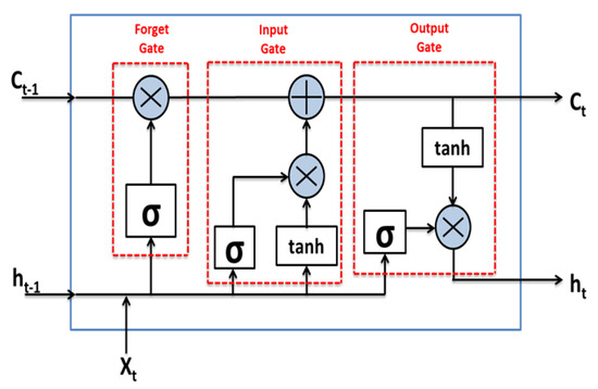
Figure 1.
General architecture of the LSTM model used in this study.
The LSTM network expects the input to be in the form of samples, time steps, and features. The structure of the LSTM model is optimized with the adjustment of the number of LSTM blocks, size of the batch, length of the input sequence, maximum of training epochs, and the number of hidden neurons. The batch size is the number of samples taken for the modification of weights, and the length of the input sequence is the time steps calculation taken for the present time step with previous ones. The more the number of hidden neurons, the better the performance of the training data. The structure of the model, as represented in Figure 2, was optimized with different hyperparameters, set with the help of the Deep Learning Toolbox in MATLAB. Although the maximum training epochs was set at 1000, the training was terminated if the validation error did not decrease during the last 50 epochs from the epoch with the minimum validation error. At the epoch when the validation error had a minimum value, the training was terminated to prevent overfitting. The data sets used for training and validation were taken from the period 2009 to 2017, whereas the data for 2018 was used for independent testing and validation. The numbers of training and validation datasets were 52,608 and 8760, respectively. With the batch size fixed at 24, we changed the sequence length (look back) of the model inputs to 6, 12, 18, 24, and 36, and the number of hidden neurons from 6 to 50 [34].
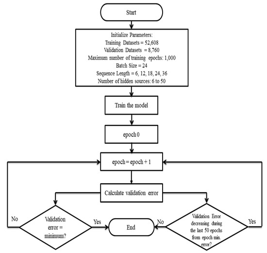
Figure 2.
Workflow diagram of the LSTM model employed in the study.
To assess the model performance, the latest version of instant computation and plotting in IRI (IRI-2016) was accessed from the Community Coordinated Modeling Center (CCMC)- NASA (https://ccmc.gsfc.nasa.gov/modelweb/models/iri2016_vitmo.php; accessed on 10 December 2021). IRI-2016 encompasses three different sub-model options (NeQuick, IRI01-corr, and IRI2001) for the topside electron density, and three different sub-model options (Bil-2000, Gul-1987, and ABT-2009) for the bottom side thickness. The recommended default options NeQuick (topside) and ABT-2009 (bottom side) were chosen in this study for estimating hourly TEC, as their overall performances appeared to be the best over equatorial and low-latitude regions [5,49].
3. Results and Discussion
The model evaluation was done by comparing the model-predicted values with the observed values of GPS-TEC and IRI-2016 model estimates. The IRI model, a widely recognized model, has often been used to estimate the prediction performances of ionosphere models. The IRI-2016 model provides empirically estimated, not forecast, values for a given time and location [34]. The LSTM model requires the previous observation data for the prediction of the present model outputs before the comparison with the observations. For the evaluation, the dataset considered days that had no more than the 14 interpolated values in the two-day sequence. For the analysis of the model, the data was randomly selected and the RMSE and correlation coefficient (CC) were calculated. Figure 3 shows the performance of the model during the training and validation phases using input and target datasets from 2009 to 2017. The training was stopped when there ceased to be any more improvement in the model performance. The low RMSEs and convergence of the training and validation datasets indicated good model performance. A dataset for the year 2018 not included in the training or validation, was used for independent testing of the LSTM model performance.
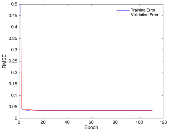
Figure 3.
LSTM model performance during training and validation with the input parameters at a low latitude station Bangalore (IISC) in India.
Figure 4 shows the hourly ionospheric TEC forecasting of the GPS, IRI, and LSTM, including the model performances, which were calculated for random days in the year 2018. The random days were chosen to verify the performance of the model, and care was taken to avoid probable cases of overfitting. It was observed that the LSTM predicted hourly values representing the diurnal TEC variation by the GPS observations better than the IRI TEC estimates in all the days randomly considered. Furthermore, we analyzed the model’s performance during geomagnetically disturbed periods in 2018, as shown in Figure 5. The geomagnetically disturbed days were selected based on the divergence of the Dst index from its reference level. It can be observed from the figure that the modeled magnitudes nearly followed the GPS-TEC for almost all the days chosen in Figure 5. However, there were a few instances where the LSTM predictions marginally underestimated or overestimated during the diurnal peak hours. As for the random quiet days, IRI predictions during geomagnetically disturbed days also deviated from the observed GPS-TEC during the daytime, with the maximal disagreement during the late afternoon hours, inferring the failure of the IRI model to appropriately align with the observed magnitudes.
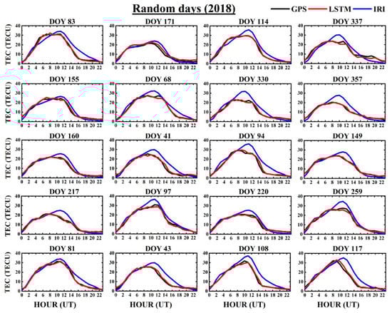
Figure 4.
Comparison of the TECs predicted for the random days of the year (DOY) in 2018 by the GPS TEC (black solid line), IRI (blue solid line), and LSTM (red solid line) at a low latitude station Bangalore (IISC) in India.
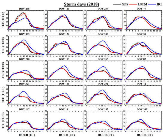
Figure 5.
Comparison of the TECs predicted for selected geomagnetically disturbed days of the year (DOY) in 2018 by the GPS TEC (black solid line), IRI (blue solid line), and LSTM (red solid line) at a low latitude station Bangalore (IISC) in India.
Figure 6 shows the model validation metrics between the LSTM and IRI TEC estimates and the GPS TEC values for the whole of the year 2018. It is evident from Figure 6, that all the error metrics (mean squared error (MSE), normalized mean squared error (NMSE), root mean squared error (RMSE), normalized root mean squared error (NRMSE), mean absolute error (MAE)), between the LSTM and GPS were minimal compared to the other models. Hence, the LSTM model effectively predicted the GPS TEC observations at the station.
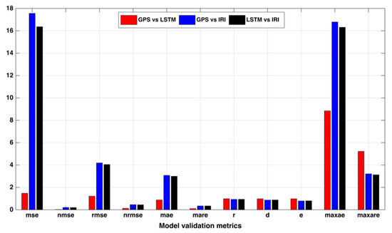
Figure 6.
Model validation metrics between GPS vs. LSTM, GPS vs. IRI, and LSTM vs. IRI at a low latitude station Bangalore (IISC) in India.
To further validate the day-to-day performance of the LSTM TEC model, the modeled and observed daily hourly TEC estimates were analyzed. Figure 7 shows a comparison of error plots and correlation coefficients of the designed model with the theoretical method and observed values for the daily prediction of the year 2018. The LSTM model closely followed the observed GPS-TEC data. The LSTM model had minimum error values, while the IRI model combination had maximum errors in the prediction of the data, relative to the observation data. The TEC variations for the year of 2018 (testing period) were considered to evaluate and compare the models with the original GPS-TEC. It is evident from Figure 7, that the LSTM model followed the observed GPS-TEC values very well during all the investigations in the test period. The correlation plot in Figure 7c shows that the LSTM model (with higher CC values) was superior, compared to the IRI model. The IRI model had higher RMSE values (2–8 TECU) compared to a combination of GPS and LSTM models. The performance of the model was higher with lower RMSE values.
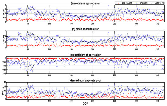
Figure 7.
Scatter plots of (a) root mean square error (RMSE), (b) mean absolute error (MAE), (c) coefficient of correlation (CC), (d) maximum absolute error of GPS vs. LSTM, GPS vs. IRI, and LSTM vs. IRI at a low latitude station Bangalore (IISC) in India.
Figure 8 depicts the scatter plot comparing the GPS-TEC values measured from GPS observations with the IRI, and LSTM values. It can be observed from Figure 8 that, rather than the IRI model, the LSTM model best fit with the GPS-measured TEC data. Moreover, the proposed deep learning model, the LSTM model, was more suitably correlated with the data, having goodness of fit (r) of 0.992 while other models had less r value compared to the LSTM model. The performance of the forecasting models could not be defined by a single measure. Thus, more performance indices were included in the complete assessment, which included separately defining the root mean square (RMSE), mean absolute error (MAE), the maximum absolute error (MAXAE), and the correlation coefficient (CC). The forecasting accuracy could be effectively assessed by the RMSE. The model performed better, as its RMSE value was smaller as time increased. In addition, as the forecasting error could be positive and negative, the MAE was the average of the absolute error, which could better reflect the definite position of the predicting value error. The degree of linear correlation between forecast value and actual value was indicated by r [20].
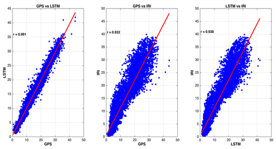
Figure 8.
Scatter plots for hourly GPS TEC and corresponding modeled TEC values using LSTM and IRI models.
In Figure 9, we represent the summary statistics of the model’s performance for the selected period. The deep learning LSTM method performed better and was closer to the GPS, compared to the traditional method IRI. The box plots visually show the distribution of numerical data and skewness, by displaying the data quartiles (or percentiles) and averages. The upper and lower quartiles are joined by lines known as whiskers. Hence, it can be termed a box and whisker plot. The box plot shows the dispersion of the data set of different models. It displays the data in five number summaries by dividing into sections, namely, minimum, first quartile, median, third quartile, and maximum. The LSTM model gave a dispersion of the data within the range of GPS. The IRI data was widely dispersed and left-skewed. Thus, the LSTM model was more precise than the IRI model in forecasting.
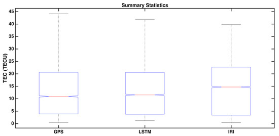
Figure 9.
Summary statistics of the TEC data for the observed GPS data with IRI and deep learning method LSTM.
In brief, the present LSTM architecture performed relatively better than the empirical IRI-2016 model at a low latitude location closer towards the magnetic equator location. However, a regional spatiotemporal forecasting of TEC through the proposed model needs further refinement to provide seamless output, irrespective of locations of observation and geomagnetic activity conditions. Earlier reports of Mannucci et al. [50], Borries et al. [51] and Tsurutani et al. [52] highlight that there are significantly large changes in the equatorial and near equatorial dayside TEC during the main phases of magnetic storms, and the forecast model may not be able to reproduce such anomalous alterations in TEC if all the drivers during the storm are not participating in the proposed model. At present, SSN, F10.7, Kp, Ap, and Dst indices were included in the LSTM model. A thorough investigation of geomagnetic storm periods is suggested to consider the underlying drivers of the equatorial and low latitude ionosphere in the model for a realistic representation of dynamic changes in TEC over the region.
4. Conclusions
In this paper, an LSTM deep learning network model was implemented for a one-day ahead ionospheric TEC forecast at a low-latitude Indian location. The observed TEC values, over the period from 2009 to 2017, were used for training the model, whereas the observed TEC for 2018 was reserved for independent training and validation. An appropriate set of solar and geomagnetic indices were chosen, along with hourly observed TEC variables, to present an optimal forecast of TEC values 24 h in advance. The performance of the LSTM ionospheric forecast model was evaluated by comparing the results with observed GPS-TEC data and IRI-2016 model estimations. The analysis of comparison among these models was carried out for one year (2018 year). The experimental performance of the proposed algorithm, LSTM, was compared with IRI and GPS models, based on error measurement metrics (RMSE = 1.6149) and coefficients of correlation (CC = 0.992) during the test period, inferring a relatively improved performance of the LSTM at the low latitude Indian location. The better performance of LSTM was attributed to its usage with the maximum goodness of fit (r) of 0.992. Therefore, a deep learning model, LSTM, may be a suitable forecast model for estimating the ionospheric parameters for GPS signals over the Indian low latitude region. The study will be extended further to refine the model by including other driving parameters, such as solar wind, to reproduce a realistic representation of the dynamic changes in TEC over the region, particularly during extreme geomagnetic and ionospheric storms. The LSTM performance can be further examined at different GPS station locations under diverse solar and geomagnetic conditions to eventually develop a regional forecast of TEC above Indian low latitudes, which is the eventual goal of this undergoing research project.
Author Contributions
Conceptualization, M.M. and S.K.P.; Formal analysis, K.D.R. and L.S.N.; Investigation, K.D.R., M.A.A., P.J. and L.S.N.; Methodology, M.M. and S.K.P.; Software, K.D.R., L.S.N., M.M. and M.A.A.; Supervision, S.K.P. and V.R.D.; Validation, V.R.D., M.A.A., P.J., M.M. and S.K.P.; Visualization, V.R.D., M.A.A., P.J., M.M. and S.K.P.; Writing—original draft, K.D.R., L.S.N. and M.M.; Writing—review and editing, V.R.D., M.A.A., P.J. and S.K.P. All authors have read and agreed to the published version of the manuscript.
Funding
This research work was supported by the Core Research Grant (CRG) scheme under the Science and Engineering Research Board (SERB) (A statutory body of the Department of Science & Technology, Government of India), New Delhi, India, under grant number CRG/2019/003394.
Institutional Review Board Statement
Not applicable.
Informed Consent Statement
Not applicable.
Data Availability Statement
The GPS observation data and broadcast ephemeris files used in this study were obtained from the Crustal Dynamics Data Information System (CDDIS) archive (https://cddis.nasa.gov/archive/gnss/, accessed on 12 September 2021). The instant run of IRI model was executed at https://ccmc.gsfc.nasa.gov/modelweb/models/iri2016_vitmo.php/, accessed on 22 December 2021.
Acknowledgments
The authors acknowledge Gopi K. Seemala for providing access to the GPS-TEC analysis program for extracting the TEC values from GPS observables and S. Moon for technical discussion on the implementation of LSTM in this study.
Conflicts of Interest
The authors declare no conflict of interest.
References
- Dubey, S.; Wahi, R.; Gwal, A.K. Ionospheric effects on GPS positioning. Adv. Space Res. 2006, 38, 2478–2484. [Google Scholar] [CrossRef]
- Kintner, P.M.; Ledvina, B.M. The ionosphere, radio navigation, and global navigation satellite systems. Adv. Space Res. 2005, 35, 788–811. [Google Scholar] [CrossRef]
- Li, Q.; Yang, D.; Fang, H. Two Hours Ahead Prediction of the TEC over China Using a Deep Learning Method. Universe 2022, 8, 405. [Google Scholar] [CrossRef]
- Dabas, R.S.; Bhuyan, P.K.; Tyagi, T.R.; Bhardwaj, R.K.; Lal, J.B. Day-to-day changes in ionospheric electron content at low latitudes. Radio Sci. 1984, 19, 749–756. [Google Scholar] [CrossRef]
- Prasad, S.N.V.S.; Rama Rao, P.V.S.; Prasad, D.S.V.V.D.; Venkatesh, K.; Niranjan, K. On the variabilities of the Total Electron Content (TEC) over the Indian low latitude sector. Adv. Space Res. 2012, 49, 898–913. [Google Scholar] [CrossRef]
- She, C.; Wan, W.; Yue, X.; Xiong, B.; Yu, Y.; Ding, F.; Zhao, B. Global ionospheric electron density estimation based on multisource TEC data assimilation. GPS Solut. 2017, 21, 1125–1137. [Google Scholar] [CrossRef]
- Cesaroni, C.; Spogli, L.; Aragon-Angel, A.; Fiocca, M.; Dear, V.; De Franceschi, G.; Romano, V. Neural network based model for global Total Electron Content forecasting. J. Space Weather Space Clim. 2020, 10, 11. [Google Scholar] [CrossRef]
- Tang, J.; Li, Y.; Ding, M.; Liu, H.; Yang, D.; Wu, X. An Ionospheric TEC Forecasting Model Based on a CNN-LSTM-Attention Mechanism Neural Network. Remote Sens. 2022, 14, 2433. [Google Scholar] [CrossRef]
- Murray, S.A. The Importance of Ensemble Techniques for Operational Space Weather Forecasting. Space Weather 2018, 16, 777–783. [Google Scholar] [CrossRef]
- Vankadara, R.K.; Panda, S.K.; Amory-Mazaudier, C.; Fleury, R.; Devanaboyina, V.R.; Pant, T.K.; Jamjareegulgarn, P.; Haq, M.A.; Okoh, D.; Seemala, G.K. Signatures of Equatorial Plasma Bubbles and Ionospheric Scintillations from Magnetometer and GNSS Observations in the Indian Longitudes during the Space Weather Events of Early September 2017. Remote Sens. 2022, 14, 652. [Google Scholar] [CrossRef]
- Ogwala, A.; Oyedokun, O.J.; Akala, A.O.; Amaechi, P.O.; Simi, K.G.; Panda, S.K.; Ogabi, C.; Somoye, E.O. Characterization of ionospheric irregularities over the equatorial and low latitude Nigeria region. Astrophys. Space Sci. 2022, 367, 79. [Google Scholar] [CrossRef]
- Xia, G.; Zhang, F.; Wang, C.; Zhou, C. ED-ConvLSTM: A Novel Global Ionospheric Total Electron Content Medium-Term Forecast Model. Space Weather 2022, 20, e2021SW002959. [Google Scholar] [CrossRef]
- Feltens, J.; Angling, M.; Jackson-Booth, N.; Jakowski, N.; Hoque, M.; Hernández-Pajares, M.; Aragón-Àngel, A.; Orús, R.; Zandbergen, R. Comparative testing of four ionospheric models driven with GPS measurements. Radio Sci. 2011, 46, RS0D12. [Google Scholar] [CrossRef]
- Seok, H.-W.; Ansari, K.; Panachai, C.; Jamjareegulgarn, P. Individual performance of multi-GNSS signals in the determination of STEC over Thailand with the applicability of Klobuchar model. Adv. Space Res. 2022, 69, 1301–1318. [Google Scholar] [CrossRef]
- Meng, X.; Mannucci, A.J.; Verkhoglyadova, O.P.; Tsurutani, B.T. On forecasting ionospheric total electron content responses to high-speed solar wind streams. J. Space Weather Space Clim. 2016, 6, A19. [Google Scholar] [CrossRef]
- Reddybattula, K.D.; Panda, S.K.; Ansari, K.; Peddi, V.S.R. Analysis of ionospheric TEC from GPS, GIM and global ionosphere models during moderate, strong, and extreme geomagnetic storms over Indian region. Acta Astronaut. 2019, 161, 283–292. [Google Scholar] [CrossRef]
- Venkatesh, K.; Fagundes, P.R.; Seemala, G.K.; de Jesus, R.; de Abreu, A.J.; Pillat, V.G. On the performance of the IRI-2012 and NeQuick2 models during the increasing phase of the unusual 24th solar cycle in the Brazilian equatorial and low-latitude sectors. J. Geophys. Res. Space Phys. 2014, 119, 5087–5105. [Google Scholar] [CrossRef]
- Chartier, A.T.; Matsuo, T.; Anderson, J.L.; Collins, N.; Hoar, T.J.; Lu, G.; Mitchell, C.N.; Coster, A.J.; Paxton, L.J.; Bust, G.S. Ionospheric data assimilation and forecasting during storms. J. Geophys. Res. Space Phys. 2016, 121, 764–778. [Google Scholar] [CrossRef]
- Xiong, P.; Zhai, D.; Long, C.; Zhou, H.; Zhang, X.; Shen, X. Long Short-Term Memory Neural Network for Ionospheric Total Electron Content Forecasting Over China. Space Weather 2021, 19, e2020SW002706. [Google Scholar] [CrossRef]
- Han, Y.; Wang, L.; Fu, W.; Zhou, H.; Li, T.; Chen, R. Machine Learning-Based Short-Term GPS TEC Forecasting During High Solar Activity and Magnetic Storm Periods. IEEE J. Sel. Top. Appl. Earth Obs. Remote Sens. 2022, 15, 115–126. [Google Scholar] [CrossRef]
- Liu, L.; Zou, S.; Yao, Y.; Wang, Z. Forecasting Global Ionospheric TEC Using Deep Learning Approach. Space Weather 2020, 18, e2020SW002501. [Google Scholar] [CrossRef]
- Dabbakuti, J.R.K.K.; Bhavya Lahari, G. Application of Singular Spectrum Analysis Using Artificial Neural Networks in TEC Predictions for Ionospheric Space Weather. IEEE J. Sel. Top. Appl. Earth Obs. Remote Sens. 2019, 12, 5101–5107. [Google Scholar] [CrossRef]
- Kaselimi, M.; Voulodimos, A.; Doulamis, N.; Doulamis, A.; Delikaraoglou, D. Deep Recurrent Neural Networks for Ionospheric Variations Estimation Using GNSS Measurements. IEEE Trans. Geosci. Remote Sens. 2022, 60, 1–15. [Google Scholar] [CrossRef]
- Xenos, T.D. Neural-network-based prediction techniques for single station modeling and regional mapping of the foF2 and M(3000)F2 ionospheric characteristics. Nonlinear Process. Geophys. 2002, 9, 477–486. [Google Scholar] [CrossRef]
- Hernández-Pajares, M.; Juan, J.M.; Sanz, J. Neural network modeling of the ionospheric electron content at global scale using GPS data. Radio Sci. 1997, 32, 1081–1089. [Google Scholar] [CrossRef]
- Maruyama, T. Retrieval of in situ electron density in the topside ionosphere from cosmic radio noise intensity by an artificial neural network. Radio Sci. 2002, 37, 10–11. [Google Scholar] [CrossRef]
- Oyeyemi, E.O.; McKinnell, L.A.; Poole, A.W.V. Near-real time foF2 predictions using neural networks. J. Atmos. Sol.-Terr. Phys. 2006, 68, 1807–1818. [Google Scholar] [CrossRef]
- Tulunay, E.; Senalp, E.T.; Radicella, S.M.; Tulunay, Y. Forecasting total electron content maps by neural network technique. Radio Sci. 2006, 41, RS4016. [Google Scholar] [CrossRef]
- Habarulema, J.B.; McKinnell, L.-A.; Cilliers, P.J.; Opperman, B.D.L. Application of neural networks to South African GPS TEC modelling. Adv. Space Res. 2009, 43, 1711–1720. [Google Scholar] [CrossRef]
- Tang, R.; Zeng, F.; Chen, Z.; Wang, J.-S.; Huang, C.-M.; Wu, Z. The Comparison of Predicting Storm-Time Ionospheric TEC by Three Methods: ARIMA, LSTM, and Seq2Seq. Atmosphere 2020, 11, 316. [Google Scholar] [CrossRef]
- Sabzehee, F.; Farzaneh, S.; Sharifi, M.A.; Akhoondzadeh, M. TEC Regional Modeling and prediction using ANN method and single frequency receiver over IRAN. Ann. Geophys. 2018, 61, GM103. [Google Scholar] [CrossRef]
- Kim, J.-H.; Kwak, Y.-S.; Kim, Y.H.; Moon, S.-I.; Jeong, S.-H.; Yun, J.Y. Regional Ionospheric Parameter Estimation by Assimilating the LSTM Trained Results Into the SAMI2 Model. Space Weather 2020, 18, e2020SW002590. [Google Scholar] [CrossRef]
- Hu, A.; Zhang, K. Using Bidirectional Long Short-Term Memory Method for the Height of F2 Peak Forecasting from Ionosonde Measurements in the Australian Region. Remote Sens. 2018, 10, 1658. [Google Scholar] [CrossRef]
- Moon, S.; Kim, Y.H.; Kim, J.-H.; Kwak, Y.-S.; Yoon, J.-Y. Forecasting the ionospheric F2 Parameters over Jeju Station (33.43° N, 126.30° E) by Using Long Short-Term Memory. J. Korean Phys. Soc. 2020, 77, 1265–1273. [Google Scholar] [CrossRef]
- Li, X.; Zhou, C.; Tang, Q.; Zhao, J.; Zhang, F.; Xia, G.; Liu, Y. Forecasting Ionospheric foF2 Based on Deep Learning Method. Remote Sens. 2021, 13, 3849. [Google Scholar] [CrossRef]
- Ren, X.; Yang, P.; Liu, H.; Chen, J.; Liu, W. Deep Learning for Global Ionospheric TEC Forecasting: Different Approaches and Validation. Space Weather 2022, 20, e2021SW003011. [Google Scholar] [CrossRef]
- Rao, T.V.; Sridhar, M.; Ratnam, D.V.; Harsha, P.B.S.; Srivani, I. A Bidirectional Long Short-Term Memory-Based Ionospheric foF2 and hmF2 Models for a Single Station in the Low Latitude Region. IEEE Geosci. Remote Sens. Lett. 2022, 19, 1–5. [Google Scholar] [CrossRef]
- Wen, Z.; Li, S.; Li, L.; Wu, B.; Fu, J. Ionospheric TEC prediction using Long Short-Term Memory deep learning network. Astrophys. Space Sci. 2021, 366, 3. [Google Scholar] [CrossRef]
- Zewdie, G.K.; Valladares, C.; Cohen, M.B.; Lary, D.J.; Ramani, D.; Tsidu, G.M. Data-Driven Forecasting of Low-Latitude Ionospheric Total Electron Content Using the Random Forest and LSTM Machine Learning Methods. Space Weather 2021, 19, e2020SW002639. [Google Scholar] [CrossRef]
- Kim, J.-H.; Kwak, Y.-S.; Kim, Y.; Moon, S.-I.; Jeong, S.-H.; Yun, J. Potential of Regional Ionosphere Prediction Using a Long Short-Term Memory Deep-Learning Algorithm Specialized for Geomagnetic Storm Period. Space Weather 2021, 19, e2021SW002741. [Google Scholar] [CrossRef]
- Srivani, I.; Siva Vara Prasad, G.; Venkata Ratnam, D. A Deep Learning-Based Approach to Forecast Ionospheric Delays for GPS Signals. IEEE Geosci. Remote Sens. Lett. 2019, 16, 1180–1184. [Google Scholar] [CrossRef]
- Ruwali, A.; Kumar, A.J.S.; Prakash, K.B.; Sivavaraprasad, G.; Ratnam, D.V. Implementation of Hybrid Deep Learning Model (LSTM-CNN) for Ionospheric TEC Forecasting Using GPS Data. IEEE Geosci. Remote Sens. Lett. 2021, 18, 1004–1008. [Google Scholar] [CrossRef]
- Sivakrishna, K.; Venkata Ratnam, D.; Sivavaraprasad, G. A Bidirectional Deep-Learning Algorithm to Forecast Regional Ionospheric TEC Maps. IEEE J. Sel. Top. Appl. Earth Obs. Remote Sens. 2022, 15, 4531–4543. [Google Scholar] [CrossRef]
- Shi, S.; Zhang, K.; Wu, S.; Shi, J.; Hu, A.; Wu, H.; Li, Y. An Investigation of Ionospheric TEC Prediction Maps Over China Using Bidirectional Long Short-Term Memory Method. Space Weather 2022, 20, e2022SW003103. [Google Scholar] [CrossRef]
- Seemala, G.K.; Valladares, C.E. Statistics of total electron content depletions observed over the South American continent for the year 2008. Radio Sci. 2011, 46, RS5019. [Google Scholar] [CrossRef]
- Wichaipanich, N.; Hozumi, K.; Supnithi, P.; Tsugawa, T. A comparison of neural network-based predictions of foF2 with the IRI-2012 model at conjugate points in Southeast Asia. Adv. Space Res. 2017, 59, 2934–2950. [Google Scholar] [CrossRef]
- Bai, H.; Fu, H.; Wang, J.; Ma, K.; Wu, T.; Ma, J. A prediction model of ionospheric foF2 based on extreme learning machine. Radio Sci. 2018, 53, 1292–1301. [Google Scholar] [CrossRef]
- Abri, R.; Harun, A. LSTM-Based Deep Learning Methods for Prediction of Earthquakes Using Ionospheric Data. Gazi Univ. J. Sci. 2022, 35, 1417–1431. [Google Scholar] [CrossRef]
- Kumar, S.; Tan, E.L.; Razul, S.G.; See, C.M.S.; Siingh, D. Validation of the IRI-2012 model with GPS-based ground observation over a low-latitude Singapore station. Earth Planets Space 2014, 66, 17. [Google Scholar] [CrossRef]
- Mannucci, A.J.; Tsurutani, B.T.; Iijima, B.A.; Komjathy, A.; Saito, A.; Gonzalez, W.D.; Guarnieri, F.L.; Kozyra, J.U.; Skoug, R. Dayside global ionospheric response to the major interplanetary events of October 29–30, 2003 “Halloween Storms”. Geophys. Res. Lett. 2005, 32, L12S02. [Google Scholar] [CrossRef]
- Borries, C.; Berdermann, J.; Jakowski, N.; Wilken, V. Ionospheric storms—A challenge for empirical forecast of the total electron content. J. Geophys. Res. Space Phys. 2015, 120, 3175–3186. [Google Scholar] [CrossRef]
- Tsurutani, B.T.; Verkhoglyadova, O.P.; Mannucci, A.J.; Saito, A.; Araki, T.; Yumoto, K.; Tsuda, T.; Abdu, M.A.; Sobral, J.H.A.; Gonzalez, W.D.; et al. Prompt penetration electric fields (PPEFs) and their ionospheric effects during the great magnetic storm of 30–31 October 2003. J. Geophys. Res. Space Phys. 2008, 113, A05311. [Google Scholar] [CrossRef]


Publisher’s Note: MDPI stays neutral with regard to jurisdictional claims in published maps and institutional affiliations. |
© 2022 by the authors. Licensee MDPI, Basel, Switzerland. This article is an open access article distributed under the terms and conditions of the Creative Commons Attribution (CC BY) license (https://creativecommons.org/licenses/by/4.0/).