Abstract
In this article, we review the status of the tension between the long-baseline accelerator neutrino experiments T2K and NOνA. The tension arises mostly due to the mismatch in the apappearance data of the two experiments. We explain how this tension arises based on and oscillation probabilities. We define the reference point of vacuum oscillation, maximal and and compute the appearance events for each experiment. We then study the effects of deviating the unknown parameters from the reference point and the compatibility of any given set of values of unknown parameters with the data from T2K and NOνA. T2K observes a large excess in the appearance event sample compared to the expected events at the reference point, whereas NOνA observes a moderate excess. The large excess in T2K dictates that be anchored at −90° and that with a preference for normal hierarchy. The moderate excess at NOνA leads to two degenerate solutions: (a) NH, , and ; (b) IH, , and . This is the main cause of tension between the two experiments. We review the status of three beyond standard model (BSM) physics scenarios, (a) non-unitary mixing, (b) Lorentz invariance violation, and (c) non-standard neutrino interactions, to resolve the tension.
1. Introduction
Neutrino oscillations have provided the first signal for physics beyond the standard model (SM). They were first proposed to explain the deficit in the solar neutrino flux observed by the pioneering Homestake experiment [1]. Oscillations between two neutrino flavours require them to mix and form two mass eigenstates. The survival probability of a neutrino with energy E and given flavour , after propagation over a distance L in vacuum, is given by:
where is the difference between the squares of the neutrino masses and is the mixing angle. In Equation (1), the units are chosen such that should be specified in eV2, L in meters, and E in MeV. The solar neutrino deficit was confirmed by the water Cerenkov detector Kamiokande [2], which detected the solar neutrinos in real time. Radio-chemical Gallium experiments, GALLEX [3], SAGE [4], and GNO [5], which were mostly sensitive to the low energy solar neutrinos, also observed a deficit. The high statistics water Cerenkov detector Super-Kamiokande [6] and the heavy water Cerenkov detector SNO [7] and Borexino [8] also have made detailed spectral measurements of the solar neutrino fluxes. Analysing the solar neutrino data in a two-flavour oscillation framework gives the oscillation parameters:
Observation of proton decay is one of the main physics motivations for the construction of water Cerenkov detectors, IMB [9,10] and Kamiokande [11,12]. The interactions of atmospheric neutrinos in the detector, especially those of and , could mimic the proton decay signal. Hence, these experiments have made a detailed study of the atmospheric neutrino interactions. They did not find any signal for proton decay, however instead observed a deficit of up-going atmospheric flux, relative to the down-going flux. It was proposed that the up-going neutrinos, which travel thousands of kilometres inside the Earth, oscillate into another flavour whereas the down-going neutrinos, which travel tens of kilometres, do not. The Super-Kamiokande experiment [13] observed a zenith angle dependence of the deficit, which is expected from neutrino oscillations. An analysis of the atmospheric neutrino data in a two-flavour oscillation framework gives the oscillation parameters:
we note that .
It is known that there are three flavours of neutrinos, , , and [14]. They mix to form three mass eigenstates, , , and , with mass eigenvalues , , and . The unitary matrix U, connecting the flavour basis to the mass basis,
is called the Pontecorvo–Maki–Nakagawa–Sakata (PMNS) matrix [15,16]. Naively, it seems desirable to label the lightest mass , the middle mass , and the heaviest mass . However, no method exists at present to directly measure these masses. What can be measured in oscillation experiments are the mixing matrix elements , where is a flavour index and j is a mass index. In particular, the three elements of the first row , , and are well measured. The labels 1, 2, and 3 are chosen such that .
Given the three masses , , and , it is possible to define two independent mass-squared differences, and . The third mass-squared difference is then . Without loss of generality, we can choose and . Since , we find that . As a result of the way the labels 1, 2, and 3 are chosen, these mass-squared differences, in principle, can be either positive or negative. Their signs have to be determined by experiments. The solar neutrinos, produced at the core of the sun, undergo forward elastic scattering as they travel through the solar matter. This scattering leads to matter effect [17,18], which modifies the solar electron neutrino survival probability . Super-Kamiokande [19] and SNO [7] have measured as a function of neutrino energy for MeV and found it to be of a constant value ≃0.3. SNO has also measured [7] the neutral current interaction rate of solar neutrinos to be consistent with predictions of the standard solar model [20]. The measurements of the Gallium experiments imply that for neutrino energies MeV. This increase in at lower solar neutrino energies can be explained only if is positive. At present, there is no definite experimental evidence for either a positive or negative sign of .
The PMNS matrix is similar to the quark mixing matrix introduced by Kobayashi and Maskawa [21]. It can be parameterised in terms of three mixing angles, , , and , and one char-parity (CP)-violating phase . The following parameterisation of the PMNS matrix is found to be the most convenient to analyse the neutrino data:
where and . Among these mixing angles, the CHOOZ experiment sets a strong upper bound on the middle angle [22]:
By combining this limit with the solar and atmospheric neutrino data, it can be shown that [23].
The mixing angles and the mass-squared differences have been determined in a series of precision experiments with man-made neutrino sources, which we briefly describe below.
- The long-baseline reactor neutrino experiment KamLAND [24] has km. At this long distance, it can observe oscillations due to the small mass-squared difference, . In the limit of neglecting in the three-flavour oscillation, the expression for the anti-neutrino survival probability reduces to an effective two-flavour expression:KamLAND measured the spectral distortion precisely. A combined analysis of KamLAND and solar neutrino data yields the results:
- The short baseline reactor neutrino experiments, Daya Bay [25], RENO [26], and DoubleCHOOZ [27], have baselines of the order of 1 km. At this distance, the oscillating term in containing is negligibly small. In this approximation, again reduces to an effective two-flavour expression:High statistics measurement from Daya Bay gives the measurement:
- The long-baseline accelerator experiment MINOS [28] has a baseline of 730 km and it measured the survival probability of the accelerator beam. For this baseline and for accelerator neutrino energies, the oscillating term in due to is negligibly small. Setting this term and to be zero in the three-flavour expression for , once again we obtain an effective two-flavour expression:MINOS data gives the results:
Note that both the short-baseline reactor neutrino experiments and long-baseline accelerator experiments as well as atmospheric neutrino data determine only the magnitude of but not its sign. Hence, we must consider both positive and negative sign possibilities in the data analysis. The case of positive is called normal hierarchy (NH) and that of negative is called an inverted hierarchy (IH). Both atmospheric neutrino data and accelerator neutrino data are functions of and they prefer . For such values, there are two possibilities: , which is called lower octant (LO) and , which is called higher octant (HO). At present, the data is not able to make a distinction between these two cases.
A number of groups have done global analysis of neutrino oscillation data from all the available sources: solar, atmospheric, reactor, and accelerator [29,30]. In Table 1, we present the latest results obtained by the nu-fit collaboration [29].

Table 1.
Neutrino oscillation parameters determine by nu-fit collaboration using global neutrino oscillation data [29].
Among the neutrino oscillation parameters, the mass-squared differences and the mixing angles (except for ) are measured to a precision of a few percent. On the other hand, the CP-violating phase still eludes measurement. In addition, we also need to resolve the issues of the sign of (also called the problem of neutrino mass hierarchy) and the octant of . Thus, there are currently three main unknowns in the three-flavour neutrino oscillation paradigm.
It can be shown that the survival probability of neutrinos, , is equal to that of the anti-neutrinos due to charge-parity-time (CPT) invariance. However, the oscillation probabilities and are not equal if there is CP violation. A measurement of the difference between these two probabilities will establish CP violation in neutrino oscillations and will also determine . While considering oscillation probabilities, in principle, we can enumerate six possibilities, with and taking two possible values other than . It can be shown that, in all six cases, the difference:
is proportional to:
where J is the Jarlskog invariant of the PMNS matrix [31].
Practically speaking, at production are not possible because there are no intense sources of . Nuclear reactors do produce copiously but their energies are in the range of a few MeV. When such oscillate into , the resultant anti-neutrinos are not energetic enough to produce by their interactions in the detector. Hence, are not practical choices. The neutrino beams produced by accelerators yield intense fluxes of . In principle, it is possible to search for CP violation by contrasting with or by contrasting with . However, the second option is much more difficult compared to the first for the reasons listed below.
- To produce in the detector, due to the interactions of , the neutrinos should have energies of tens of GeV. At these energies, the oscillation probabilities are quite small.
- Even when we have energetic-enough beams to produce in the detector, the efficiency of reconstructing these particles is very poor. Thus, the event numbers will be very limited.
- From Equation (14), we see that the charge-parity CP violating asymmetry:will be very small because the numerator is a product of two small quantities and , whereas the denominator is close to 1. Hence a measurement of this CP asymmetry requires high statistics.
Thus, the most feasible method to establish CP violation in neutrino oscillations and to determine is to measure the difference between and . The neutrinos do not require large energies to produce electrons/positrons on interacting in the detector. Thus, the neutrino beam energy can be tuned to the oscillation maximum. The produced electrons and positrons are relatively easy to identify in the detector. The dominant term in the expression for is proportional to [32]. The expression for the CP asymmetry in oscillations has the form:
which is much larger than . Thus, CP violation in these oscillations can be established with moderate statistics.
There are, however, some other difficulties to overcome before the goal of establishing CP violation in neutrino oscillations can be achieved. The matter effect, which modifies the solar neutrino oscillation probabilities, modifies and [33,34]. These modifications depend on the sign of . Since the dominant terms in these oscillation probabilities are proportional to , they are also subject to the octant ambiguity of . That is, the two oscillation probabilities, and , depend on all the three unknowns of the three-flavour neutrino oscillation parameters. In such a situation, the change in the probabilities induced by changing one of the unknowns can be compensated by changing another unknown. This leads to degenerate solutions that can explain a given set of measurements. Unravelling these degeneracies and making a distinction between the degenerate solutions requires a number of careful measurements and moderately high statistics.
In this review article, we analyse the theory of oscillation probability and parameter degeneracy in Section 2. Details of the analysis are discussed in Section 3. In Section 4, we outline the chronology of NOA and T2K data. In the same section, we also explain the results of the analysis of data from NOA and T2K in the past and present ones as well with the help of parameter degeneracy and describe the cause for the tension between the data of the two experiments. The resolution of the tension in terms of BSM physics is discussed in Section 5. A summary of the article is drawn in Section 6.
2. Oscillation Probability and Parameter Degeneracy
Two accelerator experiments, T2K [35] and NOA [36], take data with the aim of establishing CP violation as well as determining neutrino mass hierarchy and the octant of . Both experiments share the following common features.
- They aim a beam of to a far detector a few hundred kilometres away, which is at an off-axis location.
- The off-axis location leads to a sharp peak in neutrino spectrum [37], which is crucial to suppress the events, produced via the neutral current reaction , that form a large background for the oscillation signal.
- They have a near detector, a few hundred meters from the accelerator, which measures the neutrino flux accurately.
- The energy of the neutrino beam is tuned to be close to the oscillation maximum.
- They measure the two survival probabilities, and , and the oscillation probabilities and .
The survival probabilities lead to further improvement in the precision of and . A careful analysis of the oscillation probabilities can lead to the determination of three unknowns of the neutrino oscillation parameters. The crucial parameters of T2K and NOA experiments are summarised in Table 2. Note that the integrated flux of accelerator neutrinos is specified in units of protons on target (POT).
Table 2.
Summary of important information of T2K and NOA experiments.
We first begin with a discussion of the oscillation probabilities, and and describe how they vary with each of the unknown neutrino oscillation parameters. The three-flavour oscillation probability in the presence of matter effect with constant matter density can be written as [32]:
where , , and , with E being the energy of the neutrino and L being the length of the baseline. The parameter A is the Wolfenstein matter term [17], given by , where is the Fermi coupling constant and is the number density of the electrons in the matter. Anti-neutrino oscillation probability can be obtained by changing the sign of A and in Equation (16). The oscillation probability mainly depends on hierarchy (sign of ), octant of and , and precision in the value of . is enhanced if is in the lower half plane (LHP, ), and it is suppressed if is in the upper half plane (UHP, ), compared to the CP conserving values. In the following paragraph, for the sake of discussion, we will treat as a binary variable that either increases or decreases oscillation probability.
The dominant term in is proportional to . Therefore, the oscillation probability is rather small. It can be enhanced (suppressed), by for T2K and for NOA, due to the matter effect if is positive (negative). This dominant term is also proportional to . If , there can be two possible cases: (i) which will suppress , and (ii) which will enhance relative to the maximal . Since each of the unknowns can take 2 possible values, there are 8 different combinations of three unknowns. Any given value of can be reproduced by any of these eight combinations of the three unknowns with the appropriate choice of value. Thus, if the value of is not known precisely, it will lead to an eight-fold degeneracy in . Given that has been measured quite precisely, this degeneracy becomes less severe.
2.1. Hierarchy- Degeneracy
To start with, we assume that is maximal and the values of and are precisely known. With these assumptions, the only two unknowns are hierarchy and . From Table 1, we see that, according to the current measurements, whereas . Therefore, the first term in the expression of (and in ) in Equation (16) has the maximum matter effect contribution. This term is much larger than the second term and the third term is extremely small. We will neglect the third term in all further discussions.
For NH (IH), the first term in becomes larger (smaller). For , the situation is reversed. These changes in and in can be amplified or cancelled by the second term, depending on the value of . As a result of the dependence on term, () for NH is always larger (smaller) than that for IH. At the oscillation maxima, . Thus for (), the term is maximum (minimum) for and it is minimum (maximum) for . Therefore, for NH and , () is maximum (minimum) and for IH and , it is minimum (maximum). These two hierarchy- combinations, for both and , are well separated from each other. It can be shown that oscillation probability, for the NH and in the LHP, is well separated from that for the IH and in the UHP, for both neutrino and anti-neutrino. However, for the other two hierarchy- combinations, NH and in the UHP, and IH and in the LHP, and are quite close to each other, leading to hierarchy- degeneracy. This is illustrated in Figure 1, where and are plotted for the NOA experiment baseline. For these plots, we have used maximal , i.e., . The other mixing angle values are and . For the mass-squared differences, we have used and . is related with by the following equation [38]:
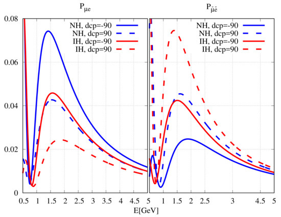
Figure 1.
(left panel) and (right panel) vs. neutrino energy for the NOA baseline. Variation of leads to the blue (red) bands for NH (IH). The plots are drawn for maximal and other neutrino parameters given in the main text.
is positive (negative) for NH (IH). For the NH and in the LHP, the values of () are reasonably greater (lower) than the values of () for the IH and any value of . Similarly, for the IH and in the UHP, the values of () are reasonably lower (greater) than the values of () for the NH and any value of . Hence, for these favourable combinations, NOA is capable of determining the hierarchy at a confidence level (C.L.) of or better, with a 3-year run each for and . However, as mentioned above, the change in the first term in Equation (16) can be cancelled by the second term for unfavourable values of . This leads to hierarchy- degeneracy [39,40,41]. From Figure 1, it can be seen that and for NH and in the UHP are very close to or degenerate with those of IH and in the LHP. For these unfavourable combinations, NOA has no hierarchy sensitivity [42]. Since the neutrino energy of T2K is only one third of the energy of NOA, the matter effect of T2K is correspondingly smaller. Therefore, T2K has very little hierarchy sensitivity. The cancellation of change due to matter effect occurs for different values of in the case of NOA and T2K. Therefore, combining the data of NOA and T2K leads to a small hierarchy discrimination capability for unfavourable hierarchy- combinations [41,42,43].
2.2. Octant-Hierarchy Degeneracy
Even though the atmospheric neutrino experiments prefer maximal (), the MINOS experiment prefers non-maximal values, [44]. The global fits, before the NOA and T2K experiment begun taking data, also favour a non-maximal value of [45,46,47], leading to two degenerate solutions: in the lower octant (LO) () and in the higher octant (HO) (). Given the two hierarchy and two octant possibilities, there are four possible octant-hierarchy combinations: LO-NH, HO-NH, LO-IH, and HO-IH. The first term of in Equation (16) becomes larger (smaller) for NH (IH). The same term also becomes smaller (larger) for LO (HO). If HO-NH (LO-IH) is the true octant-hierarchy combination, then the values of are significantly higher (smaller) than those for IH (NH) and for any octant. For these two cases, only data has good hierarchy determination capability. However, the situation is very different for the two cases LO-NH and HO-IH. The increase (decrease) in the first term of due to NH (IH) is cancelled (compensated) by the decrease (increase) for LO (HO). Therefore the two octant-hierarchy combinations, LO-NH and HO-IH, have degenerate values for . However, this degeneracy is not present in , which receives a double boost (suppression) for the case of HO-IH (LO-NH). Thus, the octant-hierarchy degeneracy in is broken by (and vice-verse). Therefore -only data has no hierarchy sensitivity if the cases LO-NH or HO-IH are true, but a combination of and data will have a good sensitivity.
This has been illustrated in Figure 2. From the figure, we can see that has degeneracy for the octant-hierarchy combinations LO-NH and HO-IH. This degeneracy does not exist in the case of [48].
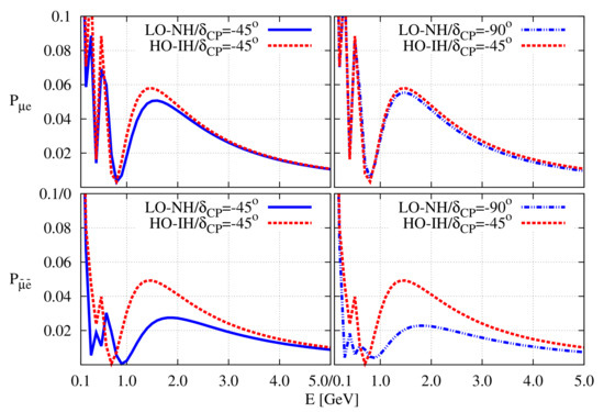
Figure 2.
Illustration of degenerate and non-degenerate for the following two cases. Left: (LO-NH, ) and (HO-IH, ). Right: (LO-NH, ) and (HO-IH, ).
2.3. Octant- Degeneracy
The possibility of two octants of also leads to octant- degeneracy. To highlight this degeneracy, we rewrite the expression for in Equation (16) as [49]:
where
In Figure 3, () is plotted for the NOA experiment as a function of neutrino energy , for normal hierarchy and for different values of . In our calculation, , when is in the LO and , when is in the HO. The has been taken equal to 0.089.
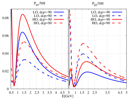
Figure 3.
as a function of neutrino energy for the NOA baseline. The left (right) panel is for (). The plots have been drawn for different possible values between and . The value is 0.089. The value of is 0.41 (0.59) for LO (HO).
From the left panel of the figure, we can see that when is in the LO and is , is quite distinctive from probability values with other and combinations. Similar arguments hold for with in the HO and . Therefore, in the LO (HO) and () is a favourable octant- combination to determine the octant of . However, for in LO and overlaps with that for in HO and . Therefore, in the LO (HO) and () is an unfavourable combination to determine the octant.
However, these unfavourable combinations become favourable for and vice-versa, as can be seen from the right panel of Figure 3. Thus, the octant- degeneracy, present in neutrino data, can be removed by anti-neutrino data and vice-versa. This aspect is different from the hierarchy- degeneracy.
The above features can also be understood by following an algebraic analysis of Equation (18). From that equation, we see that increases with the increase in . However, can increase or decrease with a change in . In the case of octant- degeneracy, for different and , we can have . It leads to:
The NOA experiment has a baseline of 810 km and the flux peaks at an energy 2 GeV. Now for the NH and neutrino,
This equation can have solutions only if:
From the above equation, we have the ranges of as:
Therefore, for the NOA experiment, for NH and neutrino, is close to [49]. Similar equations for show that this degeneracy can be removed by an anti-neutrino run.
3. Details of Data Analysis
In this section, we describe the methodology by which we have done data analyses of T2K and NOA data in Section 4 and Section 5. We have computed and between the data and a given theoretical model. In Section 4, we have discussed the evolution of NOA and T2K data with time. To do so, we have presented the analysis of the latest data from both the experiments in a standard 3-flavour oscillation scenario. In Section 5, we have discussed how different BSM scenarios alleviate the tension between the two experiments. This is done by analysing the latest data from NOA and T2K in each of the different BSM frameworks. In both Section 4 and Section 5, the results have been presented in the form of .
The observed and the expected number of events in the i-th energy bin of a given experiment are denoted by and , respectively. The between these two distributions is calculated as:
where i stands for the bins for which the observed event numbers are non-zero, j stands for bins for which the observed event numbers are zero, and z is the parameter defining systematic uncertainties.
The theoretical expected event numbers for each energy bin and the between theory and experiment have been calculated using the software GLoBES [50,51]. To do so, we fixed the signal and background efficiencies of each energy bin according to the Monte–Carlo simulations provided by the experimental collaborations [52,53,54,55]. We kept and at their best-fit values and , respectively. We varied in its range around its central value with uncertainty [56]. has been varied in its range [0.41:0.62] (with uncertainty on [57]). We varied in its range around the MINOS best-fit value with uncertainty [44]. The CP-violating phase has been varied in its complete range . In case of BSM physics, we modified the software to include new physics. The ranges of different new parameters for each of the BSM scenarios have been discussed in Section 5.
Automatic bin-based energy smearing for the generated theoretical events has been implemented within GLoBES [50,51] using a Gaussian smearing function:
where is the reconstructed energy. The energy resolution function is given by:
For NOA, we used , for electron- (muon) like events [58,59]. For T2K, we used , , for both electron- and muon-like events. For T2K, the relevant systematic uncertainties are
- A total of normalisation and energy calibration systematics uncertainty for e-like events, and
- A total of normalisation and energy calibration systematics uncertainty for -like events.
For NOA, we used normalisation and energy calibration systematic uncertainties for both the e-like and -like events [58]. Details of systematic uncertainties have been discussed in the GLoBES manual [50,51].
During the calculation of , we added (for the older, pre-2020 data) priors on , , and , in cases where we have not included muon disappearance data. In all other cases, priors have been added on only (to account for electron disappearance data from reactor neutrino experiments).
We calculated the for both the hierarchies. Once the s had been calculated, we subtracted the minimum from them to calculate the . The parameter values and hierarchy, for which the , is called the best-fit point.
4. Evolution of the Tension between NOA and T2K Data
In this section, we consider the appearance data of T2K and NOA in both modes and discuss how they give rise to degenerate solutions. We will highlight the growing tension between these appearance data when they are interpreted within the three-flavour oscillation paradigm. In the next section, we will consider new physics scenarios that can reduce that tension.
4.1. Evolution of the NOA data
In 2017, NOA published their first result with a combined analysis of appearance and disappearance data, corresponding to POT [60]. This analysis gave three solutions that were almost degenerate:
- NH, , (NH, LO, ),
- NH, , (NH, HO, ), and
- IH, , (NH, HO, ).
In Ref. [61], an effort was made to understand this degeneracy in the NOA data from 2017. To do so, the authors of Ref. [61] first calculated the expected appearance event numbers for vacuum oscillation, maximal , and for POT. This case was labelled as ‘000’. Then they considered changes in this number due to (a) matter effect, (b) octant of non-maximal , and (c) large value of . The parameter value for which is increased (decreased) was labelled as ‘+’ (‘+’). First, one change at a time was introduced in the following manner:
- NH, which increases (labelled as ‘+’) or IH, which decreases it (labelled as ‘+’),
- HO, which increases (labelled as ‘+’) or LO, which decreases it (labelled as ‘+’),
- , which increases (labelled as ‘+’) or , which decreases it (labelled as ‘+’).
The event numbers for POT were calculated using the software GLoBES [50,51]. Other parameters were fixed at following constant values: , , , , and . The values of (NH) and (IH) were taken from the analysis of NOA disappearance data. The results are presented in Table 3. From this table, it is obvious that the increase (decrease) in for any single ‘+’ (‘+’) change in the unknown parameters is essentially the same.
Table 3.
Expected appearance events of NOA for POT. They are listed for the reference point and for change of one unknown parameter at a time. NOA observed 33 appearance events in 2017.
Next all eight possible combinations in the changes of the three unknown parameters were considered. All three unknown parameters can shift in a way that each change leads to an increase in . This can be labelled as ‘’. In this case, one gains the maximum number of appearance events. Another case is that two of the unknown parameters change to increase , whereas the third one decreases it. This can happen in three possible ways, labelled as ‘’, ‘’, and ‘’. These three combinations lead to a moderate increase in appearance events compared to the reference ’000’ case. Similarly, a moderate decrease in the appearance event numbers compared to the reference case can occur due to an increase in by one unknown parameter and decrease by the other two. This can occur in three possible ways: ‘’, ‘’, and ‘’. Finally there is a possible case where each of the three changes lowers and we get the minimum number of appearance events. This can be labelled as ‘’. In Table 4, the number of appearance events for POT and for all the eight combinations, mentioned above, have been listed. From the table, we can see that the number of events for ‘’, ‘’, and ‘’ are nearly the same. A similar statement can be made about ‘’, ‘’, and ‘’. The predicted number of events for ‘’ and ‘’ are totally unique. Thus, the eight-fold degeneracy, present before the was measured, breaks itself down to the pattern after the precise measurement of . The 2017 NOA data saw a moderate increase in appearance events, compared to the expected event numbers for the reference case ’000’. Hence, there was a three-fold degeneracy in the NOA solutions. In Table 5, the expected number of appearance events for POT at each of the NOA solutions have been listed. The predictions for two NH solutions matched the experimentally observed event numbers 33. The prediction of the IH solution (which was away from the NH solutions) was lower by 3 (half the statistical uncertainty in the expected number). The occurrence of three-fold degeneracy in the NOA data, based on the inherent degeneracy in was also discussed in Ref. [62].
Table 4.
Expected appearance events of NOA for POT, and for eight different combinations of unknown parameters.
Table 5.
Expected appearance events of NOA for POT, and for the three solutions in Ref. [60].
In Ref. [61], the authors also considered the possible resolution of three-fold degeneracy with the anti-neutrino run. One can obtain the anti-neutrino oscillation probability by reversing the signs of matter term A, and in Equation (16). decreases (increases) for NH (IH). Similarly, in the UHP (LHP) increases (decreases) . However, we continue to label the NH (IH) as ‘+’ (‘+’). In the same way, in the LHP (UHP) will be labelled as ‘+’ (‘+’). However, it should be noted that the ‘+’ (‘+’) sign in the hierarchy and leads to a decrease (increase) in . Conversely, for the octant of , ‘+’ (‘+’), the sign leads to an increase (decrease) in . Now, for the ‘’ solution, decreases due to the hierarchy, and increases due to the octant of and . Similarly, for the ‘’ solution, increases due to the hierarchy and octant of , and decreases due to . Hence these two solutions are degenerate for anti-neutrino data, and the NOA appearance data would not be able to distinguish between them. However, for the third solution ‘’, decreases due to all three unknown parameters. The expected appearance events for this case would be the smallest. In principle, the NOA appearance data for POT would be able to distinguish this solution for the other two. Since the expected number of events for this particular scale is rather small, as can be seen from Table 6, the statistical uncertainty would be large, and the NOA appearance data with POT would not be able to distinguish this solution from the other two at the level.
Table 6.
Expected appearance events of NOA for POT, and for the three solutions in Ref. [60].
In the Neutrino 2018 conference, NOA published results after analysing data corresponding to () POTs in the neutrino (anti-neutrino) mode [58,63]. They found out the best-fit point at (), (), () for NH (IH). NH was preferred over IH at C.L. In addition, in the IH was excluded at more than C.L. The neutrino disappearance data were consistent with the maximal , whereas the disappearance data preferred a non-maximal mixing [64]. Therefore, there was a mild tension between the two different data sets of the same experiment. However, since the statistics from the anti-neutrino disappearance data were very low, this tension was not statistically significant. In the case of appearance data, the expected number of () appearance events at the reference point ’000’ was 39 () [64]. The observed () appearance events were 58 (18). Hence, there was a moderate excess in both these channels. As we have already seen, the moderate excess in both and appearance channels is possible when the change due to the hierarchy and cancels each other, and there is an increase in both channels induced by in the HO. We have already labelled these possibilities by (a) ‘’ and (b) ‘’. These are two of the three degenerate solutions of the previous 2017 data. The other degenerate solution of 2017 data, namely ‘’ was ruled out by 2018 data because although this solution leads to moderate excess in the appearance events, it causes a minimum number of appearance events. In Ref. [64], an analysis of the and appearance data from 2018 was performed. It was found out that there were two degenerate best-fit solutions: (i) NH, , , and (ii) IH, , . The first solution is in the form of (a) and the second solution is in the form of (b). The best-fit points given by the NOA collaboration were also in these two forms. However, because of the inclusion of the disappearance data in the analysis of the NOA collaboration, a smaller value, compared to those mentioned above, of was obtained.
In 2020, NOA published the analysis of their data corresponding to () POT in the () mode [52,53]. The best-fit points were (), (), and (). In Ref. [65], a detailed analysis of the NOA data has been done. The expected and appearance event numbers at the reference point ’000’ are and respectively. The observed event numbers in these channels are 82 and 33, respectively. Thus, there is a moderate excess in the appearance channel, and this excess can be explained by, as explained before, three possible solutions: (a) ‘’, (b) ‘’, and (c) ‘’. As for the appearance data, the observed event number 33 is consistent with the ’000’ solution. However, due to the lack of statistics in the appearance channel, other solutions are also allowed at the C.L. Exceptions are the cases labelled as ‘’, and ‘’, since these cases lead to the maximum and minimum number of expected appearance events, respectively. Thus, the solution in the form of (b) is excluded when and appearance data are analysed together. The result is shown in Figure 4. Best-fit points are of the forms (a) and (c). The best-fit points obtained by the NOA collaboration after analysing appearance and disappearance data together are of the same forms as well.
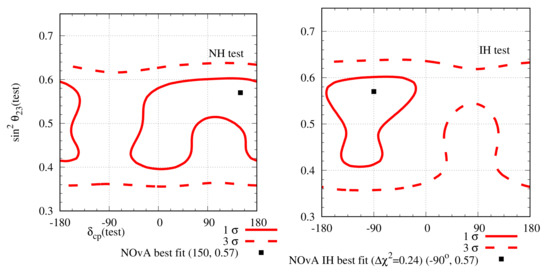
Figure 4.
Expected allowed regions in the plane from the NOA appearance data, as given in Refs. [52,53], for both the and channels. In the left (right) panel, the hierarchy is assumed to be NH (IH). The best-fit point is at NH with a minimum for 12 energy bins. IH has a minimum .
4.2. Evolution of the T2K Data
In 2013, T2K published their first analysis of appearance data corresponding to POT [66,67]. They found out their best-fit point at NH and . Both the hierarchies with in the LHP were allowed at C.L., whereas values in the UHP were disfavoured at C.L. for both hierarchies. From the disappearance data published in 2014 [67], was found to be close to the maximal mixing. In Ref. [68], a detailed analysis of the physics potential of NOA in the presence of the information from T2K data were made. It was shown that if the hierarchy and are in favourable combinations, T2K data have no effect on the hierarchy determination potential of NOA. Among the unfavourable hierarchy- combinations, T2K data picked out the correct (incorrect) solution from the two degenerate solutions allowed by the NOA data for the hierarchy being IH (NH) and in the LHP (UHP). Therefore, it was concluded that if the combination of NOA and T2K prefer IH and in the LHP as the correct solution, one needs to be careful, because the actual combination might be NH and in the LHP. We will find out that this prediction in Ref. [68] was quite accurate in the context of the latest published data from NOA and T2K.
In 2018, T2K published the analysis of their data with () POT in the neutrino (anti-neutrino) mode [69]. In Ref. [64], a detailed analysis of T2K disappearance and appearance data was done separately. It was found out that the analysis of T2K disappearance data gave the best-fit point at . The C.L. on was constrained in the range [0.43:0.6]. The constraint on was valid for all values of , since the disappearance data do not have sensitivity. As for the appearance data, it was found out that the expected appearance event number at the reference point ’000’ for the given neutrino run was found out to be 60. Inclusion of matter effect changed the number by 4, and inclusion of maximal CP violation changed the number by 11. Therefore, for NH and , the expected number was increased to 80 [64]. T2K observed 89 events. Hence, the appearance data of T2K pulled the to a value larger than . An analysis of T2K appearance data was done in Ref. [64]. The data were not included because the observed number of events in this channel was too small to have any statistical significance. The best-fit point was found to be at , although was allowed at C.L. Therefore, there was a mild tension between the T2K appearance and disappearance data. The T2K collaboration, after analysing the appearance and disappearance data together gained the best-fit point at [69]. Due to the larger statistical weight of disappearance data, the final value of was determined by the disappearance data and the final value of was found to be close to the maximal value. As a result of the large excess in the observed appearance events in T2K, the was found to be in the vicinity of . For in the UHP, the expected number of events was smaller than that at the reference point. Thus in the UHP was highly disfavoured. This data also disfavoured IH, because the corresponding matter effect reduced the number of expected events. IH with was barely allowed at C.L. [69].
In 2019, T2K published data corresponding to () POT in the neutrino (anti-neutrino) mode. The best-fit point was at , () for NH (IH) [70]. They also found out that was excluded at C.L.
In 2020, T2K published their latest data with () POT in the neutrino (anti-neutrino) mode [54,55]. The best-fit point is at (), for NH (IH). This result can be explained with the change in event number due to the change in unknown parameter values from their reference point values [65]. At the reference point ‘000’, the expected number of () appearance event is 78 (19). T2K observed 113 (15) () appearance events. The large excess in the appearance channel observed by T2K can only be explained by making the choice of unknowns to be ‘’. Choosing NH leads to only an boost and we need to have a large value in HO to explain the large excess events. However, the disappearance data limits . Given that only about boost is possible from the hierarchy and octant, has to be firmly anchored around to accommodate the large excess in the appearance channel. The appearance data see a reduction in the observed events. This reduction is consistent with the event numbers expected from the ‘’ choice of the unknowns. However, the number of events in this channel is too small to have any statistical significance. In Ref. [65], an analysis of the T2K and appearance data has been done and the result is presented in Figure 5. It is obvious that the large excess in the T2K appearance channel is responsible for being close to , and this is what leads to the tension between the NOA and T2K data.
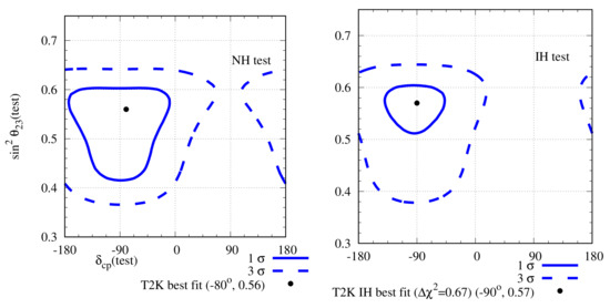
Figure 5.
Expected allowed regions in the plane from the appearance data from T2K, as given in Refs. [54,55], in both the and channels. In the left (right) panel, the hierarchy is assumed to be NH (IH). The best-fit point is at NH with a minimum for 18 energy bins.
4.3. Combined Analysis of NOA and T2K Data
Joint analyses have been planned between the NOA and T2K collaborations with the aim of obtaining better constraints on the oscillation parameters due to resolved degeneracy and to understand the non-trivial systematic correlations between them [71]. However, independent joint analyses of the two experiments have been done in Ref. [72], and it has been found out that the combined analysis prefers IH over NH. The result has been shown in Figure 6. Note that there is no overlap between the individual allowed regions of T2K and NOA. This also leads to an extremely small, , allowed region for the combined analysis.
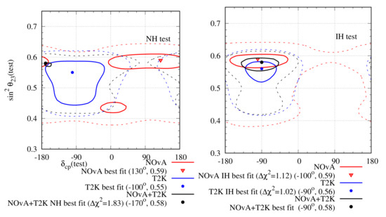
Figure 6.
Allowed region in the plane after analysing NOA and T2K complete data sets. The left (right) panel represents the test hierarchy to be NH (IH). The red (blue) lines indicate the results for NOA (T2K) and the black line indicates the combined analysis of both. The solid (dashed) lines indicate the ()-allowed regions. The minimum for NOA (T2K) with 50 (88) bins is 48.65 (95.85) and it occurs at NH. For the combined analysis, the minimum with 138 bins is 147.14, which occurs for IH.
5. Resolution of the NOA -T2K Tension with New Physics
One of the possible reasons for the tension between NOA and T2K is the existence of new physics in the neutrino oscillation. The effect of new physics on the determination of unknown oscillation parameters in the long-baseline accelerator neutrino experiments have been studied in detail in the literature [73]. In recent times, efforts have been made to resolve the tension between NOA and T2K experiments with the help of non-standard physics [74,75,76,77]. In this section, we will discuss the present status of different non-standard physics to resolve this tension.
5.1. Non-Unitary Mixing
The anomalies observed in LSND [78] and MiniBooNE [79] experiments can be explained with the existence of one or more “sterile” neutrino states with a mass at or below a few eV [80]1. The effect of sterile neutrino on the long-baseline accelerator neutrino experiments have been discussed in detail in Refs. [83,84,85,86,87]. If the sterile neutrinos exist as iso-singlet neutral heavy leptons (NHL), then in the minimum extension of the standard model, they do not take part in neutrino oscillation. However, their admixture in the charged current weak interactions affects neutrino oscillation. In such scenarios, neutrino oscillation will be governed by a non-unitary mixing matrix. The mixing matrix, in this case, can be parameterised as [88]:
Here is the standard unitary PMNS mixing matrix. The diagonal (off-diagonal) terms of the matrix are real (complex). To allow the effect of non-unitarity, the diagonal terms of the matrix must deviate from unity, and/or the off-diagonal terms must deviate from 0. The present constraints on non-unitary parameters at C.L. are [89]:
The calculation of oscillation probability in the presence of matter effect in the case of non-unitary mixing has been discussed in Refs. [74,88]. The effects of non-unitary mixing on the determination of the unknown oscillation parameters in the present and future long-baseline accelerator neutrino experiments have been discussed in the literature [88,90,91,92,93].
In the context of non-unitary mixing, the mixing between flavour states and mass eigenstates can be written as:
where denotes the flavour states and i denotes the mass eigenstates. The evolution of neutrino mass eigenstates during the propagation, can be written as:
where is the Hamiltonian in vacuum and it is defined as:
The non-unitary neutrino oscillation probability in vacuum can be written as:
If written explicitly, neglecting the cubic products of , , and , the oscillation probability takes the form [88]:
is the standard three-flavour unitary neutrino oscillation probability in vacuum and can be written as:
and
where , , and . ’s are the phases associated with the off-diagonal terms . It should be noted that non-unitary parameters , , and have the most significant effects on .
While propagating through matter, the neutrinos undergo forward scattering and the neutrino oscillation probability gets modified due to the interaction potential between the neutrino and matter. In case of non-unitary mixing, the CC and NC terms in the interaction Lagrangian is given as:
where , and are the potentials for CC and NC interactions, respectively. Therefore, the effective Hamiltonian becomes:
The non-unitary neutrino oscillation probability, after neutrinos travel through a distance L, is given as:
A detailed description of non-unitary neutrino oscillation probability in the presence of matter effect has been discussed in Ref. [74], where an effort has been made to resolve the tension between the two experiments with non-unitary mixing. To do so, the authors first analysed the present data from NOA and T2K with standard unitary oscillation hypothesis. We have already presented the result in Figure 6 using 2020 data. As mentioned in the caption of Figure 6, the minimum for NOA (T2K) is () for 50 (88) energy bins. For the combined analysis, the minimum was for 138 energy bins. In the next step, data were analysed with non-unitary mixing hypothesis. To do so, only the effects of , , and were considered, as these three parameters have the most significant effects on the oscillation probabilities , and . Only those values were chosen for which the condition [89,94] was satisfied. All other non-unitary parameters have been kept fixed at their unitary values. The software GLoBES [50,51] was used to analyse the data for both standard and non-unitary oscillations. In the later case, the software was modified to include non-unitary mixing. We have already talked about the standard unitary parameter values in Section 3. After analysing the data with non-unitary mixing hypothesis, the minimum was found to be () for NOA (T2K). For the combined analysis, the minimum was . Thus it can be said that each of the two experiments individually prefer non-unitary mixing over unitary mixing by C.L. and the combined analysis rules out unitary mixing at C.L. The result has been presented in Figure 7. It can be observed from the figure that there is a large overlap between the allowed regions of the two experiments for both the hierarchies. Both the experiments lose their hierarchy sensitivity when the data are analysed with non-unitary mixing. For the NH best-fit point, NOA (T2K) prefers to be in LO (HO), but a nearly degenerate best-fit point occurs at HO (LO). Thus, the experiments lose their octant determination sensitivity as well. Best-fit points at IH coincide for both experiments.
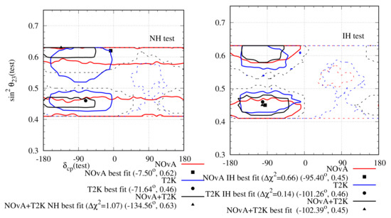
Figure 7.
Allowed region in the plane after analysing NOA and T2K complete data set with non-unitary hypothesis. The left (right) panel represents test hierarchy NH (IH). The red (blue) lines indicate the results for NOA (T2K) and the black line indicates the combined analysis of both. The solid (dashed) lines indicate the ()-allowed regions. The minimum for NOA (T2K) with 50 (88) bins is 45.88 (93.36) and it occurs at NH. For the combined analysis, the minimum with 138 bins is 142.72.
In Figure 8, as a function of individual non-unitary parameters has been represented. It is obvious that each experiment rules out unitary mixing at C.L. and the combined analysis does the same at C.L.
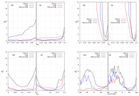
Figure 8.
as a function of individual non-unitary parameters after analysing 2020 data.
In Figure 9, we have represented the bi-event plots with the x-axis (y-axis) denoting the () appearance events. These plots are helpful in understanding the origin of the tension and their resolution with the help of new physics. As we have already seen, in NOA and T2K, all the information from appearance channels can be represented by the total number of events, and since the limited statistics, the information extracted from the shape of the energy spectrum is limited. The ellipses have been generated by fitting the combined data from NOA and T2K. The black ellipses, corresponding to the standard unitary oscillation, have been generated for the combined best-fit values of , , and . The red ellipses, corresponding to the non-unitary oscillation, have been generated for the combined best-fit values of , , and , , , , and . In both cases, only the has been varied in its complete range while keeping all other parameters fixed at their best-fit values from the combined analysis. For the black (red) ellipses, the square (circle) represent the best-fit event numbers for () for NH, and () for IH. These best-fit values come as a compromise between T2K and NOA. However, for the standard case, T2K appearance events strongly prefer NH and , and NOA prefers NH- or IH- (Table II of Ref. [65]). Thus we see that for NH, neither of the two experiments can give a good fit to the data at the combined best-fit point. A non-unitary mixing hypothesis brings the expected appearance event numbers closer to the observed event numbers. For IH, however, T2K alone cannot give a good fit to the data at the combined best-fit point for standard oscillation, and non-unitary hypothesis brings the expected event number closer to the observed event number. However, NOA can give a good fit to the data at the combined best-fit point for standard oscillation, and including non-unitary mixing does not affect it in any significant way. Hence, the tension between the two experiments is reduced by non-unitary mixing.

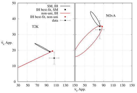
Figure 9.
Bi-event plot for T2K (NO A) in the left (right) panel. The upper (lower) panel is for NH (IH). To generate the ellipses, has been varied in the range :180 while keeping all other parameters at their combined best-fit values. The black (red) ellipses represent the SM (non-unitary) case with the best-fit points indicated by the black square (red circle). The ellipses and the best-fit points have been determined by fitting the combined data from NOA and T2K. The black circle with error bars represent the experimental data.
5.2. Lorentz Invariance Violation
Neutrino oscillation is the first experimental signature towards BSM physics, as it requires neutrinos to be massive, albeit extremely light. Without loss of any generality, SM can be considered as the low-energy effective theory derived from a more general theory–governed by the Planck mass ()–which unify the gravitational interactions along with the weak, strong, and electromagnetic interactions. There are models that include spontaneous Lorentz invariance violation (LIV) and CPT violations in that more complete framework at the Planck scale [95,96,97,98,99]. At the observable low energy, these violations can give rise to minimal extension of SM through perturbative terms suppressed by . CPT invariance imposes that particles and anti-particles have the same mass and lifetime. Observation of difference between masses and lifetimes of particles and anti-particles would be a hint of CPT violation. The present upper limit on CPT violation from the kaon system is [100]. Since kaons are bosons and the natural mass term appearing in the Lagrangian is mass squared term, the above constraints can be rewritten as . Current neutrino oscillation data provide the bounds and [101]. The non-zero differences are manifestations of some kind of CPT violation and this can change neutrino oscillation probability [102,103,104,105].
Several studies have been done about the LIV/CPT violation with neutrinos [106,107,108,109,110,111,112,113,114,115,116,117,118,119,120,121]. Different neutrino oscillation experiments have looked for LIV/CPT violations and put on constraints on the LIV/CPT violating parameters [122,123,124,125,126,127,128,129]. Constraints on all the relevant LIV/CPT violating parameters have been listed in Ref. [130]. In Ref. [75], an effort has been made to resolve the tension between NOA and T2K by considering the changes in neutrino oscillation probability due to the CPT violating LIV.
The effective Lagrangian for the Lorentz invariance-violating neutrinos and antineutrinos can be written as [102,131]:
is a dimensional spinor containing , which is a spinor field with ranging over N spinor flavours, and their charge conjugates given by . Therefore, can be expressed as:
in Equation (39) is a generic Lorentz invariance violating operator. The first term on the right side of Equation (39) is the kinetic term, the second term is the mass term involving the mass matrix M, and the third term gives rise to the LIV effect. is small and perturbative in nature.
Restricting ourselves only to the renormalizable Dirac couplings in the theory (terms only with mass dimension will be incorporated), the LIV Lagrangian in the flavour basis can be written as [102]:
where , , , and are Lorentz invariance violating parameters. Considering that only left-handed neutrinos are present in the SM, these terms can be written as:
and are constant Hermitian matrices that can modify the standard Hamiltonian in vacuum. In Ref. [75], only direction-independent isotropic terms were considered where . From now on, for simplicity, we will call terms as and the term as . involves CPT-violating terms, and involves CPT conserving Lorentz invariance violating terms. Taking into account only these isotropic LIV terms, the neutrino Hamiltonian with the LIV effect becomes:
where
Here is the Fermi coupling constant and is the electron density along the neutrino path. The in front of the second term arises due to non observability of the Minkowski trace of the CPT-conserving LIV term which relates the , , and component to the 00 component [102]. The effects of are proportional to the baseline L and the effects of are proportional to the product of energy and baseline . In Ref. [75], only the CPT-violating LIV was considered. More specifically, the authors restricted themselves to the effects of , and , because these two terms have the maximum effects on the oscillation probability [121]. The current constraint on these parameters from the Super-Kamiokande experiment at C.L. is [127]:
The oscillation probability in matter after inclusion of LIV can be approximately written as [121]:
The term in Equation (47) has been given in Equation (16). The other two terms can be written as [121]:
where ;
and
From Equation (48), it can be concluded that the LIV effects considered in this paper are matter independent. The oscillation probability for antineutrino can be calculated from Equations (16) and (48) by substituting , , and , where .
Since the effects of the CPT-violating LIV terms are proportional to L, NOA will be more sensitive to the CPT violating LIV than T2K. Thus, NOA might be sensitive to the CPT violating LIV, which T2K is insensitive to. Hence, LIV can be a possible explanation of the disagreement between the two experiments.
In Ref. [75], the individual data from NOA and T2K, as well as the combination of data from both the experiments have been analysed with LIV. As before, GLoBES [50,51] software was used to analyse the data. The software was modified to include LIV, and the oscillation probabilities and the event numbers were calculated in case of LIV without the approximations required to calculate oscillation probabilities given in Equations (47)–(50). As we have mentioned before, among the LIV parameters, only ([0:20 GeV), ([0:20 GeV), (:), and (:) have been varied. All other LIV parameters have been kept fixed to zero. The standard parameter values are just as the ones described in Section 3. We have represented the result on the plane in Figure 10. The minimum for NOA (T2K) is (). For the combined analysis, the minimum is . Both the experiments individually prefer NH as the best-fit hierarchy, although there are degenerate best-fit points at IH for both of them. The experiments lose their hierarchy sensitivity when analysed with LIV. The best-fit values of at NH are close to each other. Moreover, there is a large overlap between the -allowed regions of the two experiments. Thus, it can be concluded that the tension between the two experiments for NH has been reduced. Although, there is a new mild tension between the best-fit values of from NOA and T2K as the former prefers to be in the HO while the later prefers it to be in the LO, both of them have a degenerate best-fit point at the other octant (LO for NOA, and HO for T2K) as well. The combined experiment prefers IH over NH. However, just like the individual data, the combined data lose hierarchy (as well as octant) sensitivity and have a degenerate best-fit point at NH.
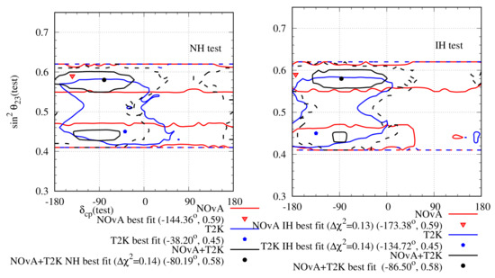
Figure 10.
Allowed region in the plane after analysing NOA and T2K complete data set with LIV hypothesis. The left (right) panel represents test hierarchy to be NH (IH). The red (blue) lines indicate the results for NOA (T2K) and the black line indicates the combined analysis of both. The solid (dashed) lines indicate the ()-allowed regions. The minimum for NOA (T2K) with 50 (88) bins is 47.71 (93.14) and it occurs at NH. For the combined analysis, the minimum with 138 bins is 145.09.
In Figure 11, we have expressed as a function of the LIV parameters. It can be seen from the figure that the present T2K data disfavours standard oscillation at C.L., whereas the NOA data do not have any preference. The combined analysis disfavours standard oscillation at C.L. as well.

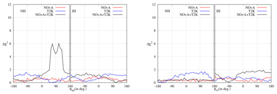
Figure 11.
as a function of individual LIV parameters.
To emphasise the result, we have presented a similar bi-event plot like Figure 9 for the non-unitary oscillation analysis in Figure 12 for the LIV analysis. It is obvious that inclusion of LIV in the theory brings the expected , and event numbers, of both experiments, at the combined best-fit point at NH closer to the observed event numbers, and thus reduces the tension between the two experiments. For IH, inclusion of LIV brings the observed , and event numbers of T2K at the combined best-fit point closer to the observed event numbers. Although, LIV takes the observed , and the event numbers of NOA at the combined IH best-fit point farther away from the observed event numbers, the change is minuscule.
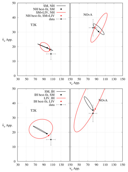
Figure 12.
Bi-event plot for T2K (NO A) in left (right) panel. The upper (lower) panel is for NH (IH). To generate the ellipses, has been varied in the range : while keeping all other parameters fixed at the combined best-fit values. The black (red) ellipses represent the SM (LIV) case with the best-fit points indicated by a black square (red circle). The ellipses and the best-fit points have been determined by fitting the combined data from NOA and T2K. The black circle with error bars represent the experimental data.
5.3. Non-Standard Interaction (NSI)
Non-standard interactions can arise as a low-energy manifestation of new heavy states of a more complete model at high energy [132,133,134,135,136] or it can arise due to light mediators [137,138]. NSI can modify the neutrino and antineutrino flavour conversion in matter [17,139,140]. The effect of NSI on the present and future long-baseline accelerator neutrino experiments have been discussed in detail in the literature [141,142,143,144,145,146]. Refs. [76,77] have tried to invoke NSI to resolve the tension between NOA and T2K data.
Neutral current NSI during neutrino propagation can be represented by a dimension 6 operator [17]:
where denote the neutrino flavour, denotes the fermions inside matter, P is the projection operator with the superscript C referring to the L or R chirality of the current, and denotes the strength of the NSI. From the hermiticity of the interaction,
For neutrino propagation through earth matter, the relevant expression is:
where is the density of f fermion. If we consider earth matter to be neutral and isoscalar, then . Thus,
The effective Hamiltonian for neutrino propagation in matter in the presence of NSI can be written in the flavour basis as:
where
It is important to note that the NC NSI Hamiltonian during propagation presented in Equations (55)–(57) are analogous to the CPT violating LIV Hamiltonian given in Equations (43)–(45). A relationship between CPT-violating LIV and NSI can be found by the following relation [147]:
The oscillation probability with matter effect in the presence of NSI during propagation can be written in a similar way as in Equation (47) [144,148,149]:
As a result of the term in Equation (60), the oscillation probability after inclusion of NSI is dependent on the matter effect unlike LIV. The first oscillation maximum of NOA (T2K) peaks at GeV ( GeV). Therefore, the matter effect is almost 3 times larger at NOA () than at T2K (). Hence, NOA can observe NSI effects which can be remain unseen by T2K. Therefore, NSI can be a possible explanation behind the tension between the two experiments.
In Refs. [76,77], an effort to resolve the tension with the NSI has been made. To do so, the authors first analysed the combined data of NOA and T2K. Finding the best-fit values of the NSI parameters after the combined analysis, they analysed the individual data from NOA and T2K with the NSI parameter values fixed at the combined best-fit values, and showed that the two experiments agree on their results on the plane. In this review article, we have analysed the individual NOA and T2K data as well as their combined data independent of each other with NSI. To do so, at first we considered only , and fixed all other NSI parameters to be 0. We presented the result on the plane in Figure 13. The minimum for NOA (T2K) with 50 (88) bins is 49.08 (93.64) and it occurs at NH (IH). For the combined analysis, the minimum with 138 bins is 146.26 and it is at NH. Both the experiments lose hierarchy sensitivity after analysing with NSI, and as a result, NOA (T2K) has a degenerate best-fit point at IH (NH). The best-fit points of the two experiments are close to each other for both the hierarchies. However, they exclude each other’s best-fit point at the C.L. for both hierarchies. There is a significant overlap between the allowed regions of the two experiments. The experiments lose their octant sensitivity as well after the inclusion of NSI. At the best-fit points, the values are close to for both the experiments and hierarchies. The combined analysis prefers NH, in HO, and as the best-fit point. However, there is a nearly degenerate best-fit point at IH, in HO, and .
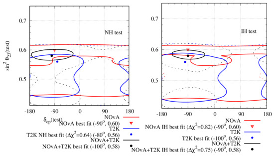
Figure 13.
Allowed region in the plane after analysing NOA and T2K complete data set with NSI hypothesis. Only the effect of has been considered. The left (right) panel represents test hierarchy to be NH (IH). The red (blue) lines indicate the results for NOA (T2K) and the black line indicates the combined analysis of both. The solid (dashed) lines indicate the ()-allowed regions. The minimum for NOA (T2K) with 50 (88) bins is 49.08 (93.64) and it occurs at NH. For the combined analysis, the minimum with 138 bins is 146.26.
Just like the non-unitary mixing and LIV, we emphasised our argument about resolution of the tension with the inclusion of NSI due to through bi-event plots presented in Figure 14. It is clear that for both the experiments, the inclusion of NSI due to brings the expected and event numbers at the combined best-fit points closer to the observed event numbers for NH, and thus resolves the tension between the two experiments for NH. For IH, the change in expected event numbers for T2K at the combined best-fit point after inclusion of NSI due to is negligible. For NOA, the expected event numbers at the combined IH best-fit point comes closer to the observed event number after inclusion of NSI due to , whereas change in the expected appearance event number due to the same is negligible.

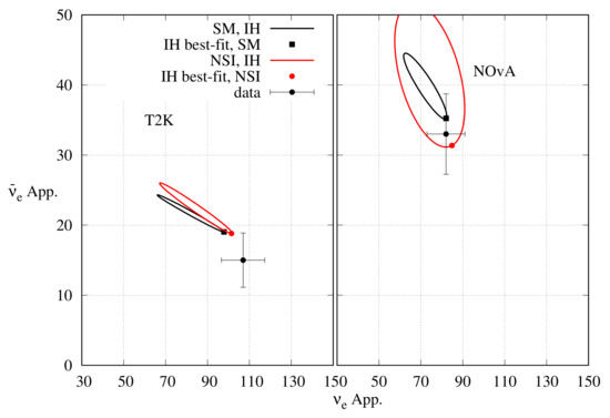
Figure 14.
Bi-event plot for T2K (NO A) in the left (right) panel. The upper (lower) panel is for NH (IH). To generate the ellipses, has been varied in the range while keeping all other parameters fixed. Among the NSI parameters, only the effect of has been considered. The black (red) ellipses represent the SM (NSI) case with the best-fit points indicated by a black square (red circle). The ellipses and best-fit points have been determined by fitting the combined data from NOA and T2K. The black circle with error bars represent the experimental data.
In the next step, we have considered the effects of . All other NSI parameters have been kept fixed at 0. The result has been displayed on the plane in Figure 15. The minimum for NOA (T2K) with 50 (88) bins is 48.59 (93.73) and it occurs at IH. For the combined analysis, the minimum with 138 bins is 146.38 and it is at NH. Although NOA and T2K both individually prefer IH and in LO as their best-fit point, both of them lose hierarchy and octant sensitivity after consideration of NSI parameter , and therefore both of them have a degenerate best-fit point at NH as well as in HO. The best-fit points of the two experiments are close to each other. However, both of them exclude each other’s best-fit point at C.L. for both the hierarchies. Nonetheless, there is a significant overlap between the -allowed region of the two experiments after including the effect of the NSI parameter . At the best-fit points, the values are close to for both the experiments and hierarchies. The combined analysis prefers NH, in HO and as the best-fit point. However, there is a nearly degenerate best-fit point at IH, in HO and .
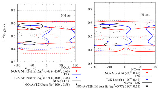
Figure 15.
Allowed region in the plane after analysing NOA and T2K complete data set with the NSI hypothesis. Only the effect of has been considered. The left (right) panel represents test hierarchy to be NH (IH). The red (blue) lines indicate the results for NOA (T2K) and the black line indicates the combined analysis of both. The solid (dashed) lines indicate the () allowed regions. The minimum for NOA (T2K) with 50 (88) bins is 48.59 (93.73) and it occurs at IH. For the combined analysis, the minimum with 138 bins is 146.38 and it is at NH.
As before, we have emphasised our argument about the resolution of the tension between NOA and T2K with the inclusion of NSI due to through bi-event plots in Figure 16. At the best-fit point of the combined analysis, the value of is . However, there is a nearly degenerate best-fit point at with . As a result of the stronger constraint against being large from IceCube data [150], we consider the combined best-fit point at . It is clear that for NH, inclusion of NSI due to brings the expected and appearance events for both the experiments at their combined best-fit point closer to the observed event numbers. For IH, the change in expected and appearance events for T2K at the combined best-fit point is negligible. For NOA, after the inclusion of NSI due to , the expected event numbers at the combined IH best-fit point comes closer to the observed event number, whereas the change in expected appearance event number due to the same condition is quite small.
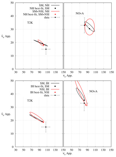
Figure 16.
Bi-event plot for T2K (NO A) in left (right) panel. The upper (lower) panel is for NH (IH). To generate the ellipses, has been varied in the range : while keeping all other parameters fixed. Among the NSI parameters, only the effect of has been considered. The black (red) ellipses represent the SM (NSI) case with the best-fit points indicated by black square (red circle). The ellipses and the best-fit points have been determined by fitting the combined data from NOA and T2K. The black circle with error bars represent the experimental data.
In Figure 17, we have presented the precision plots for the NSI parameters. It can be concluded that when we consider the effect of , the present NOA data cannot make any preference between SM and NSI. However, both T2K and the combined data rule out SM at C.L. When the effect of is considered, all three cases – NOA, T2K, and their combined data – rule out SM at C.L.
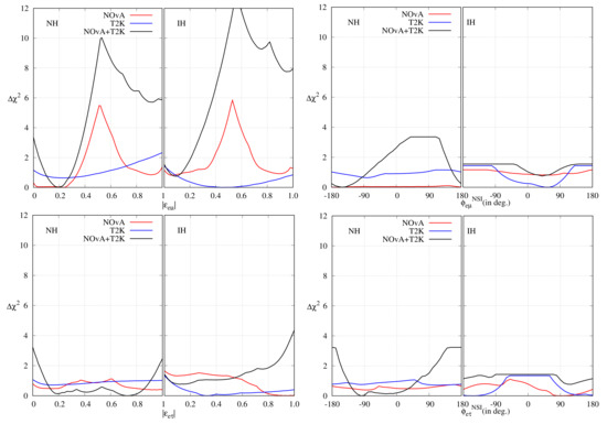
Figure 17.
as a function of individual NSI parameters.
The best-fit values for various non-standard parameters discussed in this section have been listed in Table 7. The C.L. limit for 1 degree of freedom (d.o.f.) of these parameters have been mentioned as well in the parenthesis. When the limit falls beyond the studied range of a parameter, NA has been mentioned instead of a number.
Table 7.
Best-fit values of several BSM parameters discussed in Section 5 along with the -error bar, where available. The C.L. limits for 1 d.o.f. have been mentioned in the parenthesis. When the limit falls beyond the studied range of a parameter, NA has been mentioned.
6. Summary and Discussion
A tension between the best-fit points of T2K and NOA existed from the very beginning, which became only stronger with time. This tension arises mostly from the appearance data of the two experiments. T2K observes a large excess in the appearance events compared to the expected event number at the reference point of vacuum oscillation, , and (referred to as 000). This large excess dictates that be anchored around and that be in HO, for both the hierarchies (‘’ and ‘’, with the former being the best-fit point). The appearance events observed by NOA show a very different pattern. They are moderately larger than the expectation from the reference point in the channel and are consistent with it in the channel. These two facts, when combined together, lead to two possible degenerate solutions for NO A: A. NH- in HO- in UHP (‘’), and B. IH- in HO- in LHP (‘’). A fit of the combined T2K + NOA data to a standard three-flavour oscillation framework, has the best-fit point as IH- in HO- in LHP, which is reasonably close to the IH best-fit points of T2K and NOA. If NH is assumed to be the true hierarchy, there is almost no allowed region within , despite the best-fit point of each experiment picking NH. This is the essential tension between the two experiments.
Several studies have been done to resolve this tension with BSM physics. Three different BSM scenarios have been considered in the literature: (1) Non-unitary mixing, (2) Lorentz invariance violation, and (3) non-standard interaction during neutrino propagation. All three scenarios bring the expected event numbers at the combined best-fit point at NH closer to the observed , and event numbers of both the experiments, and thus reduce the tension between them.
T2K and NOA individually prefer non-unitary mixing over unitary mixing at C.L. Combined data from both of them prefer non-unitary mixing at C.L. Both the experiments lose hierarchy and octant sensitivity when analysed with non-unitary mixing. There is a large overlap between the -allowed regions on the plane of the two experiments.
In the case of LIV, T2K data prefers LIV over standard 3-flavour oscillation at . NOA data cannot make any preference between the two hypothesis at . The combined analysis rules out standard oscillation at C.L. Similar to non-unitary mixing, both experiments lose hierarchy, and octant sensitivity in the case of LIV too. In this case, there is also a large overlap between the -allowed region on the plane of the two experiments.
In the case of NSI, we considered the effects of , and one at a time. In case of , T2K data rule out standard oscillation at C.L., whereas NOA data cannot make a preference between the two hypothesis. The combined data from NOA and T2K rule out standard oscillation at more than C.L. In the case of , data from both NOA and T2K rule out standard oscillation at , whereas their combined data rule out standard oscillation at C.L. As before, in the case of NSI also, each of the two experiments loses their hierarchy and octant sensitivity. A large overlap between the -allowed regions on the plane of the two experiments exists.
T2K and NOA continue to take data. The additional data may either sharpen or reduce the tension. If the tension becomes sharper, then we need to explore which new physics scenario can best relieve this tension. We also need to test the predictions of the preferred new physics scenario in future neutrino oscillation experiments, such as T2HK [151] and DUNE [152,153,154].
Author Contributions
Conceptualization, U.R.; methodology, U.R., S.R., S.U.S.; software, U.R.; validation, U.R., S.R. and S.U.S.; formal analysis, U.R.; investigation, U.R.; resources, S.R.; data curation, U.R.; writing—original draft preparation, U.R.; writing—review and editing, S.R., S.U.S.; visualization, S.U.S.; supervision, S.U.S.; project administration, U.R.; funding acquisition, S.R. All authors have read and agreed to the published version of the manuscript.
Funding
U.R. and S.R. were funded by the University of Johannesburg Research Council grant number RB40/3624.
Data Availability Statement
In this article, we used already available public data from the NOA and T2K collaborations. These data can be accessed from refs. [52,53,54,55].
Acknowledgments
U.R. and S.R. were supported by a grant from the Research Council of the University of Johannesburg.
Conflicts of Interest
The authors declare no conflict of interest. The funders had no role in the design of the study; in the collection, analyses, or interpretation of data; in the writing of the manuscript, or in the decision to publish the results.
Note
| 1 | Recent results from the MicroBooNE experiment [81] rule out any excess electron-like events at C.L. However, they do not rule out the complete parameter space suggested by the MiniBooNE experiment and other data, nor do they probe the interpretation of the MiniBooNE result in a model independent way [82]. |
References
- Cleveland, B.T.; Daily, T.; Davis, R., Jr.; Distel, J.R.; Lande, K.; Lee, C.K.; Wildenhain, P.S.; Ullman, J. Measurement of the solar electron neutrino flux with the Homestake chlorine detector. Astrophys. J. 1998, 496, 505–526. [Google Scholar] [CrossRef]
- Hirata, K.S.; Inoue, K.; Ishida, T.; Kajita, T.; Kihara, K.; Nakahata, M.; Nakamura, K.; Ohara, S.; Sato, N.; Suzuki, Y.; et al. Real time, directional measurement of B-8 solar neutrinos in the Kamiokande-II detector. Phys. Rev. D 1991, 44, 2241, Erratum in Phys. Rev. D 1992, 45, 2170. [Google Scholar] [CrossRef]
- Hampel, W.; Handt, J.; Heusser, G.; Kiko, J.; Kirsten, T.; Laubenstein, M.; Pernicka, E.; Rau, W.; Wojcik, M.; Zakharov, Y.; et al. GALLEX solar neutrino observations: Results for GALLEX IV. Phys. Lett. B 1999, 447, 127–133. [Google Scholar] [CrossRef]
- Abdurashitov, J.N.; Gavrin, V.N.; Gorbachev, V.V.; Gurkina, P.P.; Ibragimova, T.V.; Kalikhov, A.V.; Khairnasov, N.G.; Knodel, T.V.; Mirmov, I.N.; Shikhin, A.A.; et al. Measurement of the solar neutrino capture rate with gallium metal. III: Results for the 2002–2007 data-taking period. Phys. Rev. C 2009, 80, 015807. [Google Scholar] [CrossRef]
- Altmann, M.; Balata, M.; Belli, P.; Bellotti, E.; Bernabei, R.; Burkert, E.; Cattadori, C.; Cerulli, R.; Chiarini, M.; Cribier, M.; et al. Complete results for five years of GNO solar neutrino observations. Phys. Lett. B 2005, 616, 174–190. [Google Scholar] [CrossRef]
- Abe, K.; Haga, Y.; Hayato, Y.; Ikeda, M.; Iyogi, K.; Kameda, J.; Kishimoto, Y.; Marti, L.; Miura, M.; Moriyama, S.; et al. Solar Neutrino Measurements in Super-Kamiokande-IV. Phys. Rev. D 2016, 94, 052010. [Google Scholar] [CrossRef]
- Aharmim, B.; Ahmed, S.N.; Anthony, A.E.; Barros, N.; Beier, E.W.; Bellerive, A.; Beltran, B.; Bergevin, M.; Biller, S.D.; Boudjemline, K.; et al. Measurement of the νe and Total 8B Solar Neutrino Fluxes with the Sudbury Neutrino Observatory Phase-III Data Set. Phys. Rev. C 2013, 87, 015502. [Google Scholar] [CrossRef]
- Agostini, M.; Altenmüller, K.; Appel, S.; Atroshchenko, V.; Bagdasarian, Z.; Basilico, D.; Bellini, G.; Benziger, J.; Bonfini, G.; Bravo, D.; et al. First Simultaneous Precision Spectroscopy of pp, 7Be, and pep Solar Neutrinos with Borexino Phase-II. Phys. Rev. D 2019, 100, 082004. [Google Scholar] [CrossRef]
- Casper, D.; Becker-Szendy, R.; Bratton, C.B.; Cady, D.R.; Claus, R.; Dye, S.T.; Gajewski, W.; Goldhaber, M.; Haines, T.J.; Halverson, P.G.; et al. Measurement of atmospheric neutrino composition with IMB-3. Phys. Rev. Lett. 1991, 66, 2561–2564. [Google Scholar] [CrossRef]
- Becker-Szendy, R.; Bratton, C.B.; Casper, D.; Dye, S.T.; Gajewski, W.; Goldhaber, M.; Haines, T.J.; Halverson, P.G.; Kielczewska, D.; Kropp, W.R.; et al. The Electron-neutrino and muon-neutrino content of the atmospheric flux. Phys. Rev. D 1992, 46, 3720–3724. [Google Scholar] [CrossRef]
- Hirata, K.S.; Inoue, K.; Ishida, T.; Kajita, T.; Kihara, K.; Nakahata, M.; Nakamura, K.; Ohara, S.; Sakai, A.; Sato, N.; et al. Observation of a small atmospheric muon-neutrino/electron-neutrino ratio in Kamiokande. Phys. Lett. B 1992, 280, 146–152. [Google Scholar] [CrossRef]
- Fukuda, Y.; Hayakawa, T.; Inoue, K.; Ishida, T.; Joukou, S.; Kajita, T.; Kasuga, S.; Koshio, Y.; Kumita, T.; Matsumoto, K.; et al. Atmospheric muon-neutrino/electron-neutrino ratio in the multiGeV energy range. Phys. Lett. B 1994, 335, 237–245. [Google Scholar] [CrossRef]
- Fukuda, Y.; Hayakawa, T.; Ichihara, E.; Inoue, K.; Ishihara, K.; Ishino, H.; Itow, Y.; Kajita, T.; Kameda, J.; Kasuga, S.; et al. Evidence for oscillation of atmospheric neutrinos. Phys. Rev. Lett. 1998, 81, 1562–1567. [Google Scholar] [CrossRef]
- Steinberger, J. First results at the LEP e+e− collider. Phys. Rept. 1991, 203, 346–381. [Google Scholar] [CrossRef]
- Maki, Z.; Nakagawa, M.; Sakata, S. Remarks on the unified model of elementary particles. Prog. Theor. Phys. 1962, 28, 870–880. [Google Scholar] [CrossRef]
- Bilenky, S.M.; Pontecorvo, B. Lepton Mixing and Neutrino Oscillations. Phys. Rept. 1978, 41, 225–261. [Google Scholar] [CrossRef]
- Wolfenstein, L. Neutrino oscillations in matter. Phys. Rev. D 1978, 17, 2369–2374. [Google Scholar] [CrossRef]
- Wolfenstein, L. Neutrino Oscillations and Stellar Collapse. Phys. Rev. D 1979, 20, 2634–2635. [Google Scholar] [CrossRef]
- Abe, K.; Bronner, C.; Haga, Y.; Hayato, Y.; Ikeda, M.; Iyogi, K.; Kameda, J.; Kato, Y.; Kishimoto, Y.; Marti, L.; et al. Atmospheric neutrino oscillation analysis with external constraints in Super-Kamiokande I-IV. Phys. Rev. D 2018, 97, 072001. [Google Scholar] [CrossRef]
- Bahcall, J.N.; Pinsonneault, M.H. What do we (not) know theoretically about solar neutrino fluxes? Phys. Rev. Lett. 2004, 92, 121301. [Google Scholar] [CrossRef]
- Kobayashi, M.; Maskawa, T. CP Violation in the Renormalizable Theory of Weak Interaction. Prog. Theor. Phys. 1973, 49, 652–657. [Google Scholar] [CrossRef]
- Apollonio, M.; Baldini, A.; Bemporad, C.; Caffau, E.; Cei, F.; Declais, Y.; De Kerret, H.; Dieterle, B.; Etenko, A.; George, J.; et al. Initial results from the CHOOZ long baseline reactor neutrino oscillation experiment. Phys. Lett. B 1998, 420, 397–404. [Google Scholar] [CrossRef]
- Narayan, M.; Rajasekaran, G.; Sankar, S.U. Three flavor implications of CHOOZ result. Phys. Rev. D 1998, 58, 031301. [Google Scholar] [CrossRef]
- Araki, T.; Eguchi, K.; Enomoto, S.; Furuno, K.; Ichimura, K.; Ikeda, H.; Inoue, K.; Ishihara, K.; Iwamoto, T.; Kawashima, T.; et al. Measurement of neutrino oscillation with KamLAND: Evidence of spectral distortion. Phys. Rev. Lett. 2005, 94, 081801. [Google Scholar] [CrossRef]
- Adey, D.; An, F.P.; Balantekin, A.B.; Band, H.R.; Bishai, M.; Blyth, S.; Cao, D.; Cao, G.F.; Cao, J.; Chan, Y.L.; et al. Measurement of the Electron Antineutrino Oscillation with 1958 Days of Operation at Daya Bay. Phys. Rev. Lett. 2018, 121, 241805. [Google Scholar] [CrossRef] [PubMed]
- Bak, G.; Choi, J.H.; Jang, H.I.; Jang, J.S.; Jeon, S.H.; Joo, K.K.; Ju, K.; Jung, D.E.; Kim, J.G.; Kim, J.H.; et al. Measurement of Reactor Antineutrino Oscillation Amplitude and Frequency at RENO. Phys. Rev. Lett. 2018, 121, 201801. [Google Scholar] [CrossRef]
- Abe, Y.; Appel, S.; Abrahao, T.; Almazan, H.; Alt, C.; dos Anjos, J.C.; Barriere, J.C.; Baussan, E.; Bekman, I.; Bergevin, M.; et al. Measurement of θ13 in Double Chooz using neutron captures on hydrogen with novel background rejection techniques. J. High Energy Phys. 2016, 2016, 163. [Google Scholar] [CrossRef]
- Adamson, P.; Anghel, I.; Aurisano, A.; Barr, G.; Bishai, M.; Blake, A.; Bock, G.J.; Bogert, D.; Cao, S.V.; Castromonte, C.M.; et al. Combined analysis of νμ disappearance and νμ→νe appearance in MINOS using accelerator and atmospheric neutrinos. Phys. Rev. Lett. 2014, 112, 191801. [Google Scholar] [CrossRef]
- Esteban, I.; Gonzalez-Garcia, M.C.; Maltoni, M.; Schwetz, T.; Zhou, A. The fate of hints: Updated global analysis of three-flavor neutrino oscillations. J. High Energy Phys. 2020, 2020, 178. [Google Scholar] [CrossRef]
- de Salas, P.F.; Forero, D.V.; Gariazzo, S.; Martínez-Miravé, P.; Mena, O.; Ternes, C.A.; Tórtola, M.; Valle, J.W.F. 2020 global reassessment of the neutrino oscillation picture. J. High Energy Phys. 2021, 2021, 71. [Google Scholar] [CrossRef]
- Jarlskog, C. Commutator of the Quark Mass Matrices in the Standard Electroweak Model and a Measure of Maximal CP Violation. Phys. Rev. Lett. 1985, 55, 1039. [Google Scholar] [CrossRef] [PubMed]
- Cervera, A.; Donini, A.; Gavela, M.B.; Gomez Cadenas, J.J.; Hernandez, P.; Mena, O.; Rigolin, S. Golden measurements at a neutrino factory. Nucl. Phys. B 2000, 579, 17–55, Erratum in Nucl. Phys. B 2001, 593, 731–732. [Google Scholar] [CrossRef]
- Lipari, P. Matter effects in long baseline experiments, the flavor content of the heaviest (or lightest) neutrino and the sign of Delta m**2. Phys. Rev. D 2000, 61, 113004. [Google Scholar] [CrossRef]
- Narayan, M.; Sankar, S.U. Probing the matter term at long baseline experiments. Phys. Rev. D 2000, 61, 013003. [Google Scholar] [CrossRef]
- Itow, Y.; Kajita, T.; Kaneyuki, K.; Shiozawa, M.; Totsuka, Y.; Hayato, Y.; Ishida, T.; Ishii, T.; Kobayashi, T.; Maruyama, T.; et al. The JHF-Kamioka neutrino project. arXiv 2001, arXiv:hep-ex/hep-ex/0106019. [Google Scholar]
- Ayres, D.S.; Drake, G.R.; Goodman, M.C.; Grudzinski, J.J.; Guarino, V.J.; Talaga, R.L.; Zhao, A.; Stamoulis, P.; Stiliaris, E.; Tzanakos, G.; et al. The NOvA Technical Design Report; Office of Scientific and Technical Information: Oak Ridge, TN, USA, 2007. [CrossRef]
- McDonald, K.T. An Off-axis neutrino beam. arXiv 2001, arXiv:hep-ex/0111033. [Google Scholar]
- Nunokawa, H.; Parke, S.J.; Zukanovich Funchal, R. Another possible way to determine the neutrino mass hierarchy. Phys. Rev. D 2005, 72, 013009. [Google Scholar] [CrossRef]
- Barger, V.; Marfatia, D.; Whisnant, K. Breaking eight fold degeneracies in neutrino CP violation, mixing, and mass hierarchy. Phys. Rev. D 2002, 65, 073023. [Google Scholar] [CrossRef]
- Minakata, H.; Sugiyama, H. Exploring leptonic CP violation by reactor and neutrino superbeam experiments. Phys. Lett. B 2004, 580, 216–228. [Google Scholar] [CrossRef]
- Mena, O.; Parke, S.J. Untangling CP violation and the mass hierarchy in long baseline experiments. Phys. Rev. D 2004, 70, 093011. [Google Scholar] [CrossRef]
- Prakash, S.; Raut, S.K.; Sankar, S.U. Getting the Best Out of T2K and NOvA. Phys. Rev. D 2012, 86, 033012. [Google Scholar] [CrossRef]
- Agarwalla, S.K.; Prakash, S.; Raut, S.K.; Sankar, S.U. Potential of optimized NOvA for large θ(13) and combined performance with a LArTPC and T2K. J. High Energy Phys. 2012, 2012, 75. [Google Scholar] [CrossRef]
- Nichol, R. Final MINOS Results. In Proceedings of the Neutrino 2012 Conference, Kyoto, Japan, 3–9 June 2012; Available online: http://neu2012.kek.jp/ (accessed on 10 January 2022).
- Forero, D.; Tortola, M.; Valle, J. Global status of neutrino oscillation parameters after Neutrino-2012. Phys. Rev. D 2012, 86, 073012. [Google Scholar] [CrossRef]
- Fogli, G.L.; Lisi, E.; Marrone, A.; Montanino, D.; Palazzo, A.; Rotunno, A.M. Global analysis of neutrino masses, mixings and phases: Entering the era of leptonic CP violation searches. Phys. Rev. D 2012, 86, 013012. [Google Scholar] [CrossRef]
- Gonzalez-Garcia, M.; Maltoni, M.; Salvado, J.; Schwetz, T. Global fit to three neutrino mixing: Critical look at present precision. J. High Energy Phys. 2012, 2012, 123. [Google Scholar] [CrossRef]
- Prakash, S.; Rahaman, U.; Sankar, S.U. The need for an early anti-neutrino run of NOνA. J. High Energy Phys. 2014, 2014, 70. [Google Scholar] [CrossRef]
- Agarwalla, S.K.; Prakash, S.; Sankar, S.U. Resolving the octant of theta23 with T2K and NOvA. J. High Energy Phys. 2013, 2013, 131. [Google Scholar] [CrossRef]
- Huber, P.; Lindner, M.; Winter, W. Simulation of long-baseline neutrino oscillation experiments with GLoBES (General Long Baseline Experiment Simulator). Comput. Phys. Commun. 2005, 167, 195. [Google Scholar] [CrossRef]
- Huber, P.; Kopp, J.; Lindner, M.; Rolinec, M.; Winter, W. New features in the simulation of neutrino oscillation experiments with GLoBES 3.0: General Long Baseline Experiment Simulator. Comput. Phys. Commun. 2007, 177, 432–438. [Google Scholar] [CrossRef]
- Himmel, A. New Oscillation Results From The NOvA Experiments. In Proceedings of the Neutrino 2020, Virtual Meeting, 22 Jun–2 July 2020; Available online: https://indico.fnal.gov/event/43209/contributions/187840/attachments/130740/159597/NOvA-Oscilations-NEUTRINO2020.pdf (accessed on 10 January 2022).
- Acero, M.A.; Adamson, P.; Aliaga, L.; Anfimov, N.; Antoshkin, A.; Arrieta-Diaz, E.; Asquith, L.; Aurisano, A.; Back, A.; Backhouse, C.; et al. An Improved Measurement of Neutrino Oscillation Parameters by the NOvA Experiment. arXiv 2021, arXiv:2108.08219. [Google Scholar]
- Dunne, P. Latest Neutrino Oscillation Results From T2K. In Proceedings of the Neutrino 2020, Virtual Meeting, 22 Jun–2 July 2020; Available online: https://indico.fnal.gov/event/43209/contributions/187830/attachments/129636/159603/T2K_Neutrino2020.pdf (accessed on 10 January 2022).
- Abe, K.; Akhlaq, N.; Akutsu, R.; Ali, A.; Alt, C.; Andreopoulos, C.; Antonova, M.; Aoki, S.; Arihara, T.; Asada, Y.; et al. Improved constraints on neutrino mixing from the T2K experiment with 3.13×10²¹ protons on target. Phys. Rev. D 2021, 103, 112008. [Google Scholar] [CrossRef]
- Dohnal, T. Latest Results from the Daya Bay Experiment. In Proceedings of the 37th International Cosmic Ray Conference (ICRC2021), Berlin, Germany, 12–23 July 2021. [Google Scholar] [CrossRef]
- Esteban, I.; Gonzalez-Garcia, M.C.; Hernandez-Cabezudo, A.; Maltoni, M.; Schwetz, T. Global analysis of three-flavour neutrino oscillations: Synergies and tensions in the determination of θ23,δCP, and the mass ordering. J. High Energy Phys. 2019, 2019, 106. [Google Scholar] [CrossRef]
- Acero, M.A.; Adamson, P.; Aliaga, L.; Alion, T.; Allakhverdian, V.; Anfimov, N.; Antoshkin, A.; Arrieta-Diaz, E.; Aurisano, A.; Back, A.; et al. New constraints on oscillation parameters from νe appearance and νμ disappearance in the NOvA experiment. Phys. Rev. D 2018, 98, 032012. [Google Scholar] [CrossRef]
- Acero, M.A.; Adamson, P.; Aliaga, L.; Alion, T.; Allakhverdian, V.; Altakarli, S.; Anfimov, N.; Antoshkin, A.; Aurisano, A.; Back, A.; et al. First Measurement of Neutrino Oscillation Parameters using Neutrinos and Antineutrinos by NOvA. Phys. Rev. Lett. 2019, 123, 151803. [Google Scholar] [CrossRef]
- Adamson, P.; Aliaga, L.; Ambrose, D.; Anfimov, N.; Antoshkin, A.; Arrieta-Diaz, E.; Augsten, K.; Aurisano, A.; Backhouse, C.; Baird, M.; et al. Constraints on Oscillation Parameters from νe Appearance and νμ Disappearance in NOvA. Phys. Rev. Lett. 2017, 118, 231801. [Google Scholar] [CrossRef]
- Bharti, S.; Prakash, S.; Rahaman, U.; Uma Sankar, S. Understanding the degeneracies in NOνA data. J. High Energy Phys. 2018, 2018, 36. [Google Scholar] [CrossRef]
- Lindner, M.; Rodejohann, W.; Xu, X.J. Neutrino Parameters from Reactor and Accelerator Neutrino Experiments. Phys. Rev. D 2018, 97, 075024. [Google Scholar] [CrossRef]
- Sanchez, M. NOvA Results and Prospects. In Proceedings of the XXVIII International Conference on Neutrino Physics and Astrophysics (Neutrino 2018), Heidelberg, Germany, 4–9 June 2018; Available online: https://doi.org/10.5281/zenodo.1286758 (accessed on 10 January 2022). [CrossRef]
- Nizam, M.; Bharti, S.; Prakash, S.; Rahaman, U.; Uma Sankar, S. Tensions between the appearance data of T2K and NOνA. Mod. Phys. Lett. A 2019, 35, 2050021. [Google Scholar] [CrossRef]
- Rahaman, U.; Raut, S. On the tension between the latest \nova and T2K data. arXiv 2021, arXiv:2112.13186. [Google Scholar]
- Abe, K.; Adam, J.; Aihara, H.; Akiri, T.; Andreopoulos, C.; Aoki, S.; Ariga, A.; Ariga, T.; Assylbekov, S.; Autiero, D.; et al. Observation of Electron Neutrino Appearance in a Muon Neutrino Beam. Phys. Rev. Lett. 2014, 112, 061802. [Google Scholar] [CrossRef]
- Abe, K.; Adam, J.; Aihara, H.; Akiri, T.; Andreopoulos, C.; Aoki, S.; Ariga, A.; Ariga, T.; Assylbekov, S.; Autiero, D.; et al. Precise Measurement of the Neutrino Mixing Parameter θ23 from Muon Neutrino Disappearance in an Off-Axis Beam. Phys. Rev. Lett. 2014, 112, 181801. [Google Scholar] [CrossRef] [PubMed]
- Bharti, S.; Prakash, S.; Rahaman, U.; Sankar, S.U. Hierarchy sensitivity of NOνA in light of T2K νe appearance data. arXiv 2016, arXiv:1602.03513. [Google Scholar]
- Abe, K.; Akutsu, R.; Ali, A.; Amey, J.; Andreopoulos, C.; Anthony, L.; Antonova, M.; Aoki, S.; Ariga, A.; Ashida, Y.; et al. Search for CP Violation in Neutrino and Antineutrino Oscillations by the T2K Experiment with 2.2×10²¹ Protons on Target. Phys. Rev. Lett. 2018, 121, 171802. [Google Scholar] [CrossRef] [PubMed]
- The T2K Collaboration. Constraint on the matter–antimatter symmetry-violating phase in neutrino oscillations. Nature 2020, 580, 339–344, Erratum in Nature 2020, 583, E16. [Google Scholar] [CrossRef] [PubMed]
- Berns, L. Recent Results from T2K. In Proceedings of the 55th Rencontres de Moriond on Electroweak Interactions and Unified Theories, La Thuile, Italy, 21–28 March 2020. [Google Scholar]
- Kelly, K.J.; Machado, P.A.N.; Parke, S.J.; Perez-Gonzalez, Y.F.; Funchal, R.Z. Neutrino mass ordering in light of recent data. Phys. Rev. D 2021, 103, 013004. [Google Scholar] [CrossRef]
- Argüelles, C.A.; Aurisano, A.J.; Batell, B.; Berger, J.; Bishai, M.; Boschi, T.; Byrnes, N.; Chatterjee, A.; Chodos, A.; Coan, T.; et al. New opportunities at the next-generation neutrino experiments I: BSM neutrino physics and dark matter. Rept. Prog. Phys. 2020, 83, 124201. [Google Scholar] [CrossRef] [PubMed]
- Miranda, L.S.; Pasquini, P.; Rahaman, U.; Razzaque, S. Searching for non-unitary neutrino oscillations in the present T2K and NOνA data. Eur. Phys. J. C 2021, 81, 444. [Google Scholar] [CrossRef]
- Rahaman, U. Looking for Lorentz invariance violation (LIV) in the latest long baseline accelerator neutrino oscillation data. Eur. Phys. J. C 2021, 81, 792. [Google Scholar] [CrossRef]
- Chatterjee, S.S.; Palazzo, A. Nonstandard Neutrino Interactions as a Solution to the NOνA and T2K Discrepancy. Phys. Rev. Lett. 2021, 126, 051802. [Google Scholar] [CrossRef]
- Denton, P.B.; Gehrlein, J.; Pestes, R. CP -Violating Neutrino Nonstandard Interactions in Long-Baseline-Accelerator Data. Phys. Rev. Lett. 2021, 126, 051801. [Google Scholar] [CrossRef]
- Aguilar, A.; Auerbach, L.B.; Burman, R.L.; Caldwell, D.O.; Church, E.D.; Cochran, A.K.; Donahue, J.B.; Fazely, A.; Garvey, G.T.; Gunasingha, R.M.; et al. Evidence for neutrino oscillations from the observation of anti-neutrino(electron) appearance in a anti-neutrino(muon) beam. Phys. Rev. D 2001, 64, 112007. [Google Scholar] [CrossRef]
- Aguilar-Arevalo, A.A.; Bazarko, A.O.; Brice, S.J.; Brown, B.C.; Bugel, L.; Cao, J.; Coney, L.; Conrad, J.M.; Cox, D.C.; Curioni, A.; et al. A Search for Electron Neutrino Appearance at the Δm2∼1eV2 Scale. Phys. Rev. Lett. 2007, 98, 231801. [Google Scholar] [CrossRef] [PubMed]
- Abazajian, K.N.; Acero, M.A.; Agarwalla, S.K.; Aguilar-Arevalo, A.A.; Albright, C.H.; Antusch, S.; Arguelles, C.A.; Balantekin, A.B.; Barenboim, G.; Barger, V.; et al. Light Sterile Neutrinos: A White Paper. arXiv 2012, arXiv:1204.5379. [Google Scholar]
- Abratenko, P.; An, R.; Anthony, J.; Arellano, L.; Asaadi, J.; Ashkenazi, A.; Balasubramanian, S.; Baller, B.; Barnes, C.; Barr, G.; et al. Search for Neutrino-Induced Neutral Current Δ Radiative Decay in MicroBooNE and a First Test of the MiniBooNE Low Energy Excess Under a Single-Photon Hypothesis. arXiv 2021, arXiv:2110.00409. [Google Scholar]
- Argüelles, C.A.; Esteban, I.; Hostert, M.; Kelly, K.J.; Kopp, J.; Machado, P.A.N.; Martinez-Soler, I.; Perez-Gonzalez, Y.F. MicroBooNE and the νe Interpretation of the MiniBooNE Low-Energy Excess. arXiv 2021, arXiv:2111.10359. [Google Scholar]
- Gupta, S.; Matthews, Z.M.; Sharma, P.; Williams, A.G. The Effect of a Light Sterile Neutrino at NOνA and DUNE. Phys. Rev. D 2018, 98, 035042. [Google Scholar] [CrossRef]
- Chatla, A.; Rudrabhatla, S.; Bambah, B.A. Degeneracy Resolution Capabilities of NOνA and DUNE in the Presence of Light Sterile Neutrino. Adv. High Energy Phys. 2018, 2018, 2547358. [Google Scholar] [CrossRef]
- Choubey, S.; Dutta, D.; Pramanik, D. Measuring the Sterile Neutrino CP Phase at DUNE and T2HK. Eur. Phys. J. 2018, C78, 339. [Google Scholar] [CrossRef]
- Choubey, S.; Dutta, D.; Pramanik, D. Imprints of a light Sterile Neutrino at DUNE, T2HK and T2HKK. Phys. Rev. D 2017, 96, 056026. [Google Scholar] [CrossRef]
- Berryman, J.M.; de Gouvêa, A.; Kelly, K.J.; Kobach, A. Sterile neutrino at the Deep Underground Neutrino Experiment. Phys. Rev. D 2015, 92, 073012. [Google Scholar] [CrossRef]
- Escrihuela, F.J.; Forero, D.V.; Miranda, O.G.; Tortola, M.; Valle, J.W.F. On the description of nonunitary neutrino mixing. Phys. Rev. D 2015, 92, 053009, Erratum in Phys. Rev. D 2016, 93, 119905. [Google Scholar] [CrossRef]
- Escrihuela, F.J.; Forero, D.V.; Miranda, O.G.; Tórtola, M.; Valle, J.W.F. Probing CP violation with non-unitary mixing in long-baseline neutrino oscillation experiments: DUNE as a case study. New J. Phys. 2017, 19, 093005. [Google Scholar] [CrossRef]
- Ge, S.F.; Pasquini, P.; Tortola, M.; Valle, J.W.F. Measuring the leptonic CP phase in neutrino oscillations with nonunitary mixing. Phys. Rev. D 2017, 95, 033005. [Google Scholar] [CrossRef]
- Soumya, C.; Rukmani, M. Non-unitary lepton mixing in an inverse seesaw and its impact on the physics potential of long-baseline experiments. J. Phys. G 2018, 45, 095003. [Google Scholar] [CrossRef]
- Fong, C.S.; Minakata, H.; Nunokawa, H. Non-unitary evolution of neutrinos in matter and the leptonic unitarity test. J. High Energy Phys. 2019, 2019, 15. [Google Scholar] [CrossRef]
- Verma, S.; Bhardwaj, S. Probing Non-unitary CP Violation effects in Neutrino Oscillation Experiments. Indian J. Phys. 2018, 92, 1161–1167. [Google Scholar] [CrossRef]
- Antusch, S.; Fischer, O. Non-unitarity of the leptonic mixing matrix: Present bounds and future sensitivities. J. High Energy Phys. 2014, 2014, 94. [Google Scholar] [CrossRef]
- Kostelecky, V.A.; Samuel, S. Spontaneous Breaking of Lorentz Symmetry in String Theory. Phys. Rev. D 1989, 39, 683. [Google Scholar] [CrossRef]
- Kostelecky, V.A.; Samuel, S. Phenomenological Gravitational Constraints on Strings and Higher Dimensional Theories. Phys. Rev. Lett. 1989, 63, 224. [Google Scholar] [CrossRef]
- Kostelecky, V.A.; Potting, R. CPT and strings. Nucl. Phys. B 1991, 359, 545–570. [Google Scholar] [CrossRef]
- Kostelecky, V.A.; Potting, R. CPT, strings, and meson factories. Phys. Rev. D 1995, 51, 3923–3935. [Google Scholar] [CrossRef] [PubMed]
- Kostelecky, V.A.; Potting, R. Expectation values, Lorentz invariance, and CPT in the open bosonic string. Phys. Lett. B 1996, 381, 89–96. [Google Scholar] [CrossRef]
- Tanabashi, M.; Hagiwara, K.; Hikasa, K.; Nakamura, K.; Sumino, Y.; Takahashi, F.; Tanaka, J.; Agashe, K.; Aielli, G.; Amsler, C.; et al. Review of Particle Physics. Phys. Rev. D 2018, 98, 030001. [Google Scholar] [CrossRef]
- Ohlsson, T.; Zhou, S. Extrinsic and Intrinsic CPT Asymmetries in Neutrino Oscillations. Nucl. Phys. B 2015, 893, 482–500. [Google Scholar] [CrossRef]
- Kostelecky, V.A.; Mewes, M. Lorentz and CPT violation in neutrinos. Phys. Rev. D 2004, 69, 016005. [Google Scholar] [CrossRef]
- Diaz, J.S.; Kostelecky, A. Lorentz- and CPT-violating models for neutrino oscillations. Phys. Rev. D 2012, 85, 016013. [Google Scholar] [CrossRef]
- Kostelecky, V.A.; Mewes, M. Lorentz violation and short-baseline neutrino experiments. Phys. Rev. D 2004, 70, 076002. [Google Scholar] [CrossRef]
- Katori, T.; Kostelecky, V.A.; Tayloe, R. Global three-parameter model for neutrino oscillations using Lorentz violation. Phys. Rev. D 2006, 74, 105009. [Google Scholar] [CrossRef]
- Dighe, A.; Ray, S. CPT violation in long baseline neutrino experiments: A Three flavor analysis. Phys. Rev. D 2008, 78, 036002. [Google Scholar] [CrossRef]
- Barenboim, G.; Lykken, J.D. MINOS and CPT-violating neutrinos. Phys. Rev. D 2009, 80, 113008. [Google Scholar] [CrossRef]
- Rebel, B.; Mufson, S. The Search for Neutrino-Antineutrino Mixing Resulting from Lorentz Invariance Violation using neutrino interactions in MINOS. Astropart. Phys. 2013, 48, 78–81. [Google Scholar] [CrossRef]
- De Gouvêa, A.; Kelly, K.J. Neutrino vs. Antineutrino Oscillation Parameters at DUNE and Hyper-Kamiokande. Phys. Rev. D 2017, 96, 095018. [Google Scholar] [CrossRef]
- Barenboim, G.; Ternes, C.A.; Tórtola, M. Neutrinos, DUNE and the world best bound on CPT invariance. Phys. Lett. B 2018, 780, 631–637. [Google Scholar] [CrossRef]
- Barenboim, G.; Masud, M.; Ternes, C.A.; Tórtola, M. Exploring the intrinsic Lorentz-violating parameters at DUNE. Phys. Lett. B 2019, 788, 308–315. [Google Scholar] [CrossRef]
- Majhi, R.; Chembra, S.; Mohanta, R. Exploring the effect of Lorentz invariance violation with the currently running long-baseline experiments. Eur. Phys. J. C 2020, 80, 364. [Google Scholar] [CrossRef]
- Giunti, C.; Laveder, M. Hint of CPT Violation in Short-Baseline Electron Neutrino Disappearance. Phys. Rev. D 2010, 82, 113009. [Google Scholar] [CrossRef]
- Datta, A.; Gandhi, R.; Mehta, P.; Sankar, S.U. Atmospheric neutrinos as a probe of CPT and Lorentz violation. Phys. Lett. B 2004, 597, 356–361. [Google Scholar] [CrossRef][Green Version]
- Chatterjee, A.; Gandhi, R.; Singh, J. Probing Lorentz and CPT Violation in a Magnetized Iron Detector using Atmospheric Neutrinos. J. High Energy Phys. 2014, 2014, 45. [Google Scholar] [CrossRef]
- Singh Koranga, B.; Khurana, P. CPT Violation in Atmospheric Neutrino Oscillation: A Two Flavour Matter Effects. Int. J. Theor. Phys. 2014, 53, 3737–3743. [Google Scholar] [CrossRef]
- Diaz, J.S.; Schwetz, T. Limits on CPT violation from solar neutrinos. Phys. Rev. D 2016, 93, 093004. [Google Scholar] [CrossRef]
- Hooper, D.; Morgan, D.; Winstanley, E. Lorentz and CPT invariance violation in high-energy neutrinos. Phys. Rev. D 2005, 72, 065009. [Google Scholar] [CrossRef]
- Tomar, G.; Mohanty, S.; Pakvasa, S. Lorentz Invariance Violation and IceCube Neutrino Events. J. High Energy Phys. 2015, 2015, 22. [Google Scholar] [CrossRef]
- Liao, J.; Marfatia, D. IceCube’s astrophysical neutrino energy spectrum from CPT violation. Phys. Rev. D 2018, 97, 041302. [Google Scholar] [CrossRef]
- Kumar Agarwalla, S.; Masud, M. Can Lorentz invariance violation affect the sensitivity of deep underground neutrino experiment? Eur. Phys. J. C 2020, 80, 716. [Google Scholar] [CrossRef]
- Auerbach, L.B.; Burman, R.L.; Caldwell, D.O.; Church, E.D.; Cochran, A.K.; Donahue, J.B.; Fazely, A.R.; Garvey, G.T.; Gunasingha, R.; Imlay, R.L.; et al. Tests of Lorentz violation in ν¯μ→ν¯e oscillations. Phys. Rev. D 2005, 72, 076004. [Google Scholar] [CrossRef]
- Adamson, P.; Andreopoulos, C.; Arms, K.E.; Armstrong, R.; Auty, D.J.; Ayres, D.S.; Baller, B.; Barr, G.; Barrett, W.L.; Becker, B.R.; et al. Testing Lorentz Invariance and CPT Conservation with NuMI Neutrinos in the MINOS Near Detector. Phys. Rev. Lett. 2008, 101, 151601. [Google Scholar] [CrossRef]
- Adamson, P.; Ayres, D.S.; Barr, G.; Bishai, M.; Blake, A.; Bock, G.J.; Boehnlein, D.J.; Bogert, D.; Cao, S.V.; Cavanaugh, S.; et al. Search for Lorentz invariance and CPT violation with muon antineutrinos in the MINOS Near Detector. Phys. Rev. D 2012, 85, 031101. [Google Scholar] [CrossRef]
- Aguilar-Arevalo, A.A.; Brown, B.C.; Bugel, L.; Cheng, G.; Conrad, J.M.; Cooper, R.L.; Dharmapalan, R.; Diaz, A.; Djurcic, Z.; Finley, D.A.; et al. Significant Excess of ElectronLike Events in the MiniBooNE Short-Baseline Neutrino Experiment. Phys. Rev. Lett. 2018, 121, 221801. [Google Scholar] [CrossRef]
- Abe, Y.; Aberle, C.; Dos Anjos, J.C.; Bergevin, M.; Bernstein, A.; Bezerra, T.J.C.; Bezrukhov, L.; Blucher, E.; Bowden, N.S.; Buck, C.; et al. First Test of Lorentz Violation with a Reactor-based Antineutrino Experiment. Phys. Rev. D 2012, 86, 112009. [Google Scholar] [CrossRef]
- Abe, K.; Haga, Y.; Hayato, Y.; Ikeda, M.; Iyogi, K.; Kameda, J.; Kishimoto, Y.; Miura, M.; Moriyama, S.; Nakahata, M.; et al. Test of Lorentz invariance with atmospheric neutrinos. Phys. Rev. D 2015, 91, 052003. [Google Scholar] [CrossRef]
- The IceCube Collaboration. Neutrino Interferometry for High-Precision Tests of Lorentz Symmetry with IceCube. Nat. Phys. 2018, 14, 961–966. [Google Scholar] [CrossRef]
- Abe, K.; Amey, J.; Andreopoulos, C.; Antonova, M.; Aoki, S.; Ariga, A.; Assylbekov, S.; Autiero, D.; Ban, S.; Barbato, F.C.; et al. Search for Lorentz and CPT violation using sidereal time dependence of neutrino flavor transitions over a short baseline. Phys. Rev. D 2017, 95, 111101. [Google Scholar] [CrossRef]
- Kostelecky, V.A.; Russell, N. Data Tables for Lorentz and CPT Violation. arXiv 2008, arXiv:0801.0287. [Google Scholar]
- Kostelecky, A.; Mewes, M. Neutrinos with Lorentz-violating operators of arbitrary dimension. Phys. Rev. D 2012, 85, 096005. [Google Scholar] [CrossRef]
- Farzan, Y.; Tortola, M. Neutrino oscillations and Non-Standard Interactions. Front. Phys. 2018, 6, 10. [Google Scholar] [CrossRef]
- Biggio, C.; Blennow, M.; Fernandez-Martinez, E. General bounds on non-standard neutrino interactions. J. High Energy Phys. 2009, 2009, 90. [Google Scholar] [CrossRef]
- Ohlsson, T. Status of non-standard neutrino interactions. Rept. Prog. Phys. 2013, 76, 044201. [Google Scholar] [CrossRef]
- Miranda, O.G.; Nunokawa, H. Non standard neutrino interactions: Current status and future prospects. New J. Phys. 2015, 17, 095002. [Google Scholar] [CrossRef]
- Bhupal Dev, P.S.; Babu, K.S.; Denton, P.B.; Machado, P.A.N.; Arguelles, C.A.; Barrow, J.L.; Chatterjee, S.S.; Chen, M.-C.; de Gouvea, A.; Dutta, B.; et al. Neutrino Non-Standard Interactions: A Status Report. In Proceedings of the NTN Workshop on Neutrino Non-Standard Interactions, St. Louis, MO, USA, 29–31 May 2019. [Google Scholar] [CrossRef]
- Farzan, Y. A model for large non-standard interactions of neutrinos leading to the LMA-Dark solution. Phys. Lett. B 2015, 748, 311–315. [Google Scholar] [CrossRef]
- Farzan, Y.; Shoemaker, I.M. Lepton Flavor Violating Non-Standard Interactions via Light Mediators. J. High Energy Phys. 2016, 2016, 33. [Google Scholar] [CrossRef]
- Mikheev, S.P.; Smirnov, A.Y. Resonance Amplification of Oscillations in Matter and Spectroscopy of Solar Neutrinos. Sov. J. Nucl. Phys. 1985, 42, 913–917, reprinted in Yad. Fiz. 1985, 42, 1441–1448.. [Google Scholar]
- Mikheev, S.P.; Smirnov, A.Y. Resonant amplification of neutrino oscillations in matter and solar neutrino spectroscopy. Nuovo Cim. C 1986, 9, 17–26. [Google Scholar] [CrossRef]
- Friedland, A.; Shoemaker, I.M. Searching for Novel Neutrino Interactions at NOvA and Beyond in Light of Large θ13. arXiv 2012, arXiv:1207.6642. [Google Scholar]
- Rahman, Z.; Dasgupta, A.; Adhikari, R. The Discovery reach of CP violation in neutrino oscillation with non-standard interaction effects. J. Phys. G 2015, 42, 065001. [Google Scholar] [CrossRef]
- Coelho, J.A.B.; Kafka, T.; Mann, W.A.; Schneps, J.; Altinok, O. Constraints for non-standard interaction ϵeτVe from νe appearance in MINOS and T2K. Phys. Rev. D 2012, 86, 113015. [Google Scholar] [CrossRef]
- Masud, M.; Roy, S.; Mehta, P. Correlations and degeneracies among the NSI parameters with tunable beams at DUNE. Phys. Rev. D 2019, 99, 115032. [Google Scholar] [CrossRef]
- Deepthi, K.N.; Goswami, S.; Nath, N. Challenges posed by non-standard neutrino interactions in the determination of δCP at DUNE. Nucl. Phys. B 2018, 936, 91–105. [Google Scholar] [CrossRef]
- Blennow, M.; Choubey, S.; Ohlsson, T.; Pramanik, D.; Raut, S.K. A combined study of source, detector and matter non-standard neutrino interactions at DUNE. J. High Energy Phys. 2016, 2016, 90. [Google Scholar] [CrossRef]
- Diaz, J.S. Correspondence between nonstandard interactions and CPT violation in neutrino oscillations. arXiv 2015, arXiv:1506.01936. [Google Scholar]
- Kikuchi, T.; Minakata, H.; Uchinami, S. Perturbation Theory of Neutrino Oscillation with Nonstandard Neutrino Interactions. J. High Energy Phys. 2009, 2009, 114. [Google Scholar] [CrossRef]
- Agarwalla, S.K.; Chatterjee, S.S.; Palazzo, A. Degeneracy between θ23 octant and neutrino non-standard interactions at DUNE. Phys. Lett. B 2016, 762, 64–71. [Google Scholar] [CrossRef]
- Ehrhardt, T. Search for NSI in neutrino propagation with IceCube DeepCore. In Proceedings of the 4th Uppsala workshop on Particle Physics with Neutrino Telescopes (PPNT19), Uppsala, Sweden, 7–9 October 2019; Available online: https://indico.uu.se/event/600/contributions/1024/attachments/1025/1394/IceCube_NSI_Search_PPNT19.pdf (accessed on 10 January 2022).
- The Hyper-Kamiokande Proto-Collaboration. Physics potentials with the second Hyper-Kamiokande detector in Korea. Prog. Theor. Exp. Phys. 2018, 2018, 063C01. [Google Scholar] [CrossRef]
- DUNE Collaboration. The DUNE Far Detector Interim Design Report, Volume 2: Single-Phase Module. arXiv 2018, arXiv:1807.10327. [Google Scholar]
- Abi, B.; Acciarri, R.; Acero, M.A.; Adamowski, M.; Adams, C.; Adams, D.; Adamson, P.; Adinolfi, M.; Ahmad, Z.; Albright, C.H.; et al. The DUNE Far Detector Interim Design Report Volume 1: Physics, Technology and Strategies. arXiv 2018, arXiv:1807.10334. [Google Scholar]
- Abi, B.; Bansal, S.; Friedland, A.; Kocaman, B.; Djurcic, Z.; Goudzovski, E.; Rakotondravohitra, L.; Salukvadze, G.; Mazzucato, E.; Densham, C.; et al. The DUNE Far Detector Interim Design Report, Volume 3: Dual-Phase Module. arXiv 2018, arXiv:1807.10340. [Google Scholar]


Publisher’s Note: MDPI stays neutral with regard to jurisdictional claims in published maps and institutional affiliations. |
© 2022 by the authors. Licensee MDPI, Basel, Switzerland. This article is an open access article distributed under the terms and conditions of the Creative Commons Attribution (CC BY) license (https://creativecommons.org/licenses/by/4.0/).