Abstract
We investigate the emergent time scenario in quantum cosmology based on the Page–Wotters approach. Using a quantum cosmological model with a qubit clock, it is demonstrated how the entanglement between the qubit clock and the geometry derives emergence of a time parameter, which defines evolution of the timeless quantum state of the universe. We show that the universe wave function conditioned by a qubit clock obeys the standard Schrödinger equation and the Fisher information for the clock state, which quantifies entanglement between the universe and the clock, and contributes as a negative energy density.
1. Introduction
In the canonical approach to quantum mechanics, one supposes existence of classical time as an external parameter used by the observer. The quantum state of the target system obeys the time dependent Schrödinger equation. The apparent lack of external time for the dynamics of canonical quantum gravity, described by the so-called “problem of time”, is represented by the Wheeler–DeWitt (WDW) equation [1]
for the quantum state of the universe . This equation implies the diffeomorphism invariance of the physical state, and owing to this structure, the physical state loses a concept of evolution with respect to a time parameter. Among several approaches to resolve the problem of time [2], one idea of extracting dynamics from a seemingly stationary system has been proposed, called the Page–Wotters approach or the conditional probability interpretation [3,4]. Let us consider a bipartite system composed of an universe system with the Hamiltonian and a clock system with the Hamiltonian . In the Page–Wotters approach, “time” evolution is read, under the condition that the total state Hamiltonian
is constrained, in the quantum correlation between bipartitions of the total system, the universe state (U) and the clock state (C) entangled with it. Time evolution emerges from the measurement of an observable clock of some kind, whose reading conditions the physical state.
In our previous study [5], this scenario was investigated using a Friedman–Lemaitre–Robertson–Walker (FLRW) model with a minimal scalar field. Regarding the energy eigenstate of the scalar field as a system of quantum clock, the wave function of the universe conditioned by the clock is obtained. The effect of the geometry (universe) on the clock state is encoded in the Berry phase of the scalar field state. We investigated the condition for the emergence of the standard Schrödinger equation for the universe wave function conditioned by the scalar clock. The equation contains the Berry connection, which reflects strength of a coupling between the universe and the clock, and its behavior is also related to emergence of time and entanglement between the universe and the clock. We considered several cases of the clock states with superposition of energy eigenstates and discussed a condition of workable clock. However, we did not investigate so much about entanglement property in the Page–Wotters approach. In this article, we revisit this problem using a qubit as a quantum clock in cosmology. This model is simpler than the scalar field model and captures an essential feature of the Page–Wooters mechanism. We can explicitly evaluate entanglement between the qubit clock and the universe, and discuss relation between the emergence of time and the clock-system entanglement in the timeless quantum cosmology.
The reminder of this paper is organized as follows. In Section 2, we introduce our quantum cosmological model with a qubit. In Section 3, review how the qubit operates as a quantum clock. In Section 4, we demonstrate how the qubit clock defines the time in the universe, and relation to the clock-universe entanglement is discussed in Section 5. Section 6 is devoted to summary. We adopt units of throughout this paper.
2. Mini-Superspace Model with a Qubit
We consider a spatially flat FLRW universe with a qubit clock. The metric is
where is the lapse function and is the scalar factor. We introduce the physical volume of the universe as a dynamical variable, where V denotes the comoving volume. The total Hamiltonian is written as
where
with . is the Hamiltonian for the flat FLRW universe with the spatial volume and the cosmological constant . is the Hamiltonian for the qubit with two internal energy eigenstates with the energy gap . The total Hamiltonian is constrained to be zero , and the physical state of the total system obeys the WDW equation:
where and . Here, to make clear the structure of the total state, we adopted the notation for a pure state in a bipartite Hilbert space, which is the tensor product of the universe Hilbert space and the qubit Hilbert space:
.
Let us introduce the wave function of the universe with the eigen-vector of . Then, the wave function obeys
For ,
The solution which is regular at is
where is the confluence hypergeometric function and its asymptotic behavior for is
Applying this formula, asymptotic form of the wave function for is given by
From the behavior of phase factors of the solution, the wave function represents superposition of expanding and contracting universes with the qubit energy . From the WDW Equation (10), the contribution of the qubit to the total matter energy density is proportional to , which is the same behavior as a dust fluid.
3. Clock Dynamics
Let us first consider the clock dynamics of which Hamiltonian is given by . Using the energy eigen basis of the qubit, the clock state is represented as
where we assume that the evolution of the clock state is parameterized by a time parameter T, and the state is assumed to obey the standard Schrödinger equation:
.
For the state (14),
and the solution is
where and are constants with . Probabilities to realize states and are
These probabilities oscillate with a period and the amplitude . This oscillatory behavior reflects superposition of two energy eigenstates and (interference visibility), and plays a role of a “clock”. As a special case of the state, a state with or corresponds to the energy eigenstate; the visibility becomes zero and the system does not work as a clock because we cannot measure the oscillatory behavior of the clock state.
In the cosmological situation where the clock is coupled to the external universe, constants can be functions of the spatial volume of the universe . We assume the following dependence in :
where is an arbitrary function representing a relative phase between and . The clock state is parameterized by as
.
Regarding as an external parameter, the quantum Fisher information [6,7] of this state is given by
where . This quantity is related to the distance or overlap between two states and . The Bures distance between clock states is defined by
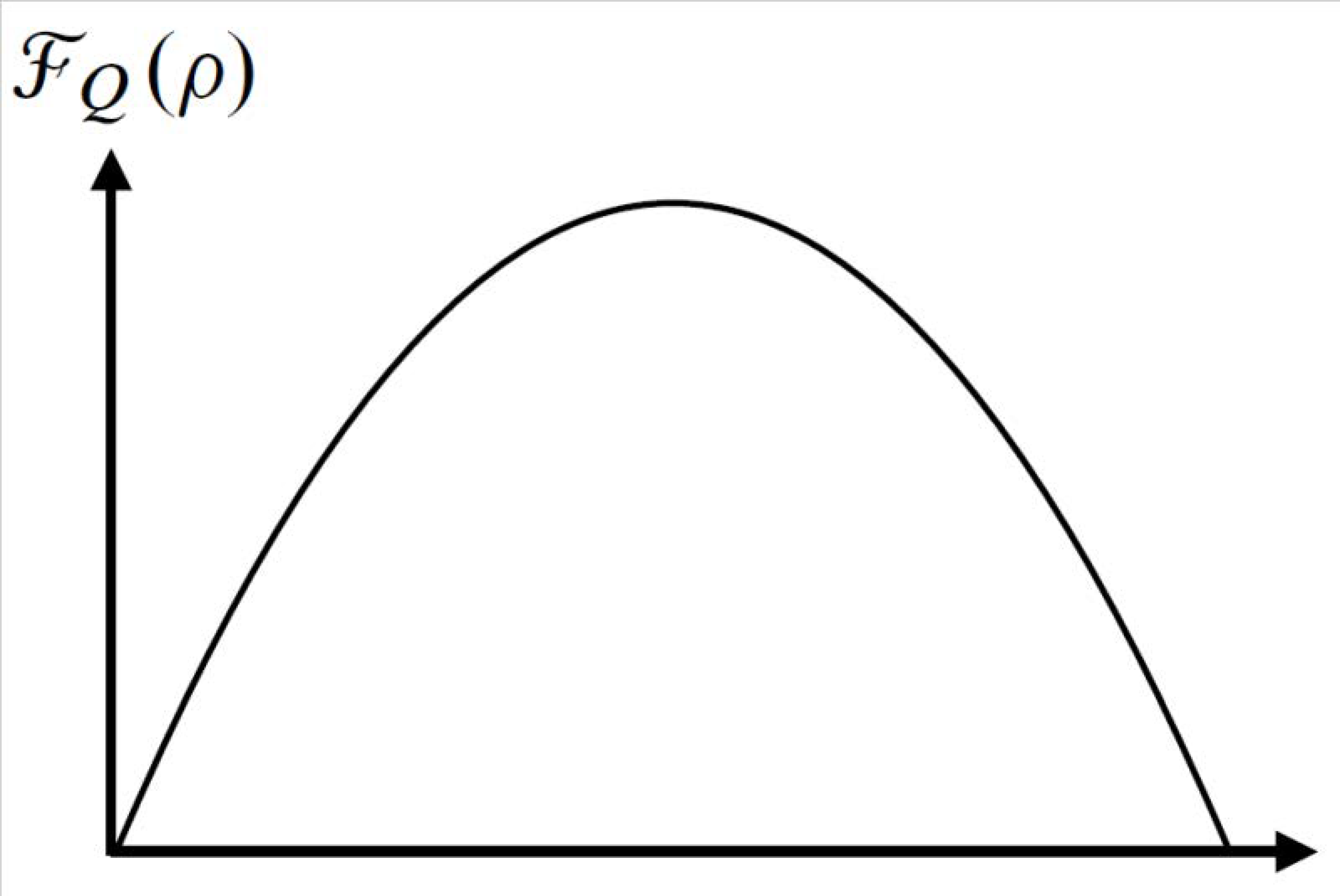
The distance between two states is proportional to the Fisher information, and becomes zero for . Figure 1 shows the behavior of the quantum Fisher information as a function of for . corresponds to the energy eigenstate, and the Fisher information is zero. Figure 1 shows dependence of the Fisher information.
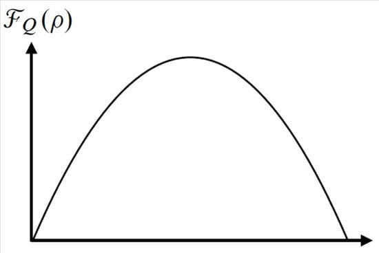
Figure 1.
Behavior of the quantum Fisher information as a function of a . For , the state is the energy eigenstate and the Fisher information becomes zero.
The Fisher information provides the Gramer–Rao bound [8], which gives a lower bound for the variance of the estimation of the external parameter :
On the other hand, using the Schrödinger Equation (15), the variance of the clock energy is expressed as
and the Cramer–Rao inequality becomes . Thus, by introducing a quantity , we obtain the following uncertainty relation between and :
The variance represents the accuracy of the clock reading. If the clock state is an energy eigenstate, then and becomes infinite, which means that the qubit system does not properly operate as a clock. Thus, for , the requirement for workable clock is , or equivalently
This is the same condition that the state is not energy eigenstate [9]. The maximum accuracy of the clock is achieved for .
4. Quantum Cosmology with a Qubit Clock
To investigate how the qubit clock introduces a time parameter in the universe, we define a wave function conditioned by the clock state (30):
where and . Then, using the WDW Equation (10), it can be shown that the wave function obeys the following equation:
It is possible to rewrite this equation to the following form:
where the covariant derivative is introduced as with the Berry connection
In this case, the Berry connection represents impact of the external parameter on the clock state . Equation (32) is invariant under the local gauge transformation , which reflects the gauge invariance of the total state. Now, we choose the “zero connection” gauge to make the equation simpler. The condition for of this gauge is
The wave function with the zero connection gauge obeys
and the coefficient of the right-hand side of this equation is
After all, the wave function satisfies
where the quantum Fisher information of the clock state appears in the right-hand side after the gauge transformation. In the left-hand side of Equation (37), using Equation (16),
where using (20) and (21). Therefore, we obtain the following Schrödinger equation for the wave function of the universe , which represents time evolution of the wave function of the universe conditioned by the qubit clock:
In deriving this equation, we should keep in mind that the condition of workable clock (29) is assumed; if this condition is not fulfilled, the clock state becomes the energy eigenstate. Then, the T-dependence included in the phase of disappears, and relevant information of time evolution of the universe is lost. In this case, the original timeless WDW Equation (10) is recovered:
where the plus and minus signs correspond to the positive () and negative () energy eigenstate of the clock, respectively.
In the right-hand side of Equation (39), represents the contribution of the qubit to matter energy density, which shows the same behavior as the classical dust fluid. On the other hand, the Fisher information contributes as a matter field with negative energy density because the Fisher information is positive semi-definite.
5. Entanglement
We evaluate entanglement between the qubit and the universe to confirm how the emergence of time due to the Page–Wotters mechanism is related to entanglement. As defined in (30), the total state conditioned by the clock is written as
The density matrix of this state is
By tracing out the qubit degrees of freedom, the reduced state is
and
where we do not specify explicit normalization of the wave function. Then, the purity is
where the overlap of two clock states is written as
with . Equality in Equation (45) is attained when the reduced system is pure state, in which case the qubit and the universe is separable (product state). As we have shown in (24) and (25), the condition of for is equivalent to and is the energy eigenstate. In this case, and the reduced system becomes pure. This implies that there is no entanglement between the qubit and the universe for . The qubit system does not work as a clock for the universe.
On the other hand, for case, and the reduced system becomes a mixed state. In this case, the qubit and the universe are entangled, and the universe wave function is parameterized by the time introduced by the qubit. The entanglement can be quantified using the mixedness, which is proportional to as shown by (46) in the present model. As presented in Equation (24), the Fisher information shows the same dependence, the Fisher information is an quantifier of the entanglement between the clock and the universe in the present model. The maximal entanglement is achieved for .
6. Summary
Using a qubit clock, we demonstrate the Page–Wotters mechanism in quantum cosmology, which explains emergence of time in timeless stationary quantum systems. The essence of this mechanism is entanglement between a clock degrees of freedom and the target system; the information of the clock system is mediated by entanglement and transferred to the timeless universe. We considered the condition of a workable qubit clock and show that the condition is non-zero values of the quantum Fisher information for the qubit state, which regards volume of the universe as an external parameter. As the qubit-universe system is totally constrained, non-zero Fisher information of the qubit system implies that the universe is capable of acquiring information of the qubit system via entanglement between the qubit and the universe. As shown in Equation (39), the Fisher information quantifies the strength of entanglement, and modifies the expansion law of the quantum universe because it serves as a negative energy density of which -dependence is determined through .
Recently, quantum nature of gravity is paid much attention from the viewpoint of quantum information [10,11]; by regarding gravitational interaction as a quantum channel, it inevitably introduces entanglement between a probe system and a target system. In the treatment of canonical quantization of gravity, owing to the WDW equation, entanglement between matter fields and gravity is encoded as universal way, and this structure is independent of detail of matter fields. Therefore, the emergent time scenario in the canonical quantum gravity is deeply related to quantum informational nature of gravity.
Funding
This work was supported in part by JSPS KAKRNHI Grant No. 19K03866.
Acknowledgments
The author would like to thank Y. Kaku, S. Maeda and Y. Osawa for useful discussion on quantumness of gravity. Preliminary idea of this study was obtained through communication with them.
Conflicts of Interest
The authors declare no conflict of interest.
References
- DeWitt, B.S. Quantum theory of gravity. I. the canonical theory. Phys. Rev. 1967, 160, 1113–1148. [Google Scholar] [CrossRef] [Green Version]
- Kiefer, C. Quantum Gravity; Oxford University Press: Oxford, UK, 2012. [Google Scholar]
- Page, D.N.; Wootters, W.K. Evolution without evolution: Dynamics described by stationary observables. Phys. Rev. D 1983, 27, 2885–2892. [Google Scholar] [CrossRef]
- Wootters, W.K. “Time” replaced by quantum correlations. Int. J. Theor. Phys. 1984, 23, 701–711. [Google Scholar] [CrossRef]
- Rotondo, M.; Nambu, Y. Clock Time in Quantum Cosmology. Universe 2019, 5, 66. [Google Scholar] [CrossRef] [Green Version]
- Paris, M.G.A. Quantum Estimation for Quantum Technology. Int. J. Quantum Inf. 2009, 7 (Suppl. 1), 125–137. [Google Scholar] [CrossRef]
- Li, N.; Luo, S. Entanglement detection via quantum Fisher information. Phys. Rev. A 2013, 88, 014301. [Google Scholar] [CrossRef]
- Braunstein, S.L.; Caves, C.M. Statistical Distance and the Geometry of Quantum States. Phys. Rev. Lett. 1994, 72, 3439–3443. [Google Scholar] [CrossRef] [PubMed]
- Anandan, J.; Aharonov, Y. Geometry of quantum evolution. Phys. Rev. Lett. 1990, 65, 1697–1700. [Google Scholar] [CrossRef] [PubMed]
- Bose, S.; Mazumdar, A.; Morley, G.W.; Ulbricht, H.; Toroš, M.; Paternostro, M.; Geraci, A.A.; Barker, P.F.; Kim, M.S.; Milburn, G. Spin Entanglement Witness for Quantum Gravity. Phys. Rev. Lett. 2017, 119, 240401. [Google Scholar] [CrossRef] [PubMed] [Green Version]
- Marletto, C.; Vedral, V. Witness gravity’s quantum side in the lab. Nature 2017, 547, 156–158. [Google Scholar] [CrossRef] [PubMed] [Green Version]
Publisher’s Note: MDPI stays neutral with regard to jurisdictional claims in published maps and institutional affiliations. |
© 2022 by the author. Licensee MDPI, Basel, Switzerland. This article is an open access article distributed under the terms and conditions of the Creative Commons Attribution (CC BY) license (https://creativecommons.org/licenses/by/4.0/).