Theory and Phenomenology of a Four-Dimensional String–Corrected Black Hole

Abstract

We construct an effective four-dimensional string-corrected black hole (4D SCBH) by rescaling the string coupling parameter in a D-dimensional Callan–Myers–Perry black hole. From the theoretical point of view, the most interesting findings are that the string corrections coincide with the so-called generalized uncertainty principle (GUP) corrections to black hole solutions, Bekenstein–Hawking entropy acquires logarithmic corrections, and that there exists a critical value of the coupling parameter for which the black hole temperature vanishes. We also find that, due to the string corrections, the nature of the central singularity may be altered from space-like to time-like singularity. In addition, we study the possibility of testing such a black hole with astrophysical observations. Since the dilaton field does not decouple from the metric, it is not a priori clear that the resulting 4D SCBH offers only small corrections to the Schwarzschild black hole. We used motion of the S2 star around the black hole at the center of our galaxy to constrain the parameters (the string coupling parameter and ADM mass) of the 4D SCBH. To test the weak gravity regime, we calculate the deflection angle in this geometry and apply it to gravitational lensing. To test the strong field regime, we calculate the black hole shadow radius. While we find that the observables change as we change the string coupling parameter, the magnitude of the change is too small to distinguish it from the Schwarzschild black hole. With the current precision, to the leading order terms, the 4D SCBH cannot be distinguished from the Schwarzschild black hole.

1. Introduction

Black holes (BHs), as the most interesting solution of Einstein’s equations, are unique objects that can provide us with both theoretical and phenomenological tests of our new models. Today, we have numerous ways to test black hole physics on astrophysical scales in both weak and strong gravity regimes. Different observational techniques using either gravitational waves or photons in practically every segment of the electromagnetic spectrum allow us to study black hole mergers, formation, shadows, accretion disk processes, gravitational lensing, star disruption process due to the presence of a black holes and so on [1,2,3]. These tests often put very strong constraints on any modification of general relativity.

While general relativity has been successfully tested on solar system scales, it does appear to run into problems at galactic and larger scales where we are forced to postulate the existence of exotic components like dark mater and dark energy. We also know that general relativity is incomplete since it is a classical theory and cannot describe space-time at the microscopic scales. The best developed candidate that might provide us with quantum description of gravity is string theory. However, making any testable prediction of the string theory proved to be notoriously difficult. Thus, any headway in this direction, albeit not quite conclusive, might be very important for further development of the field.

In this work, we consider the D-dimensional ${\alpha }^{\prime }$-corrected (where ${\alpha }^{\prime }$ is the string coupling constant) black hole found by Callan, Myers and Perry (CMP) [4]. Originally, the CMP solution was found perturbatively, with only leading order stringy corrections. Nonetheless, such a solution is important since it can give us many important insights about Hawking evaporation and related information loss paradox. This black hole solution has attracted a great deal of attention from the theoretical point of view, and was even recently used to study some potentially observational effects like the quasinormal modes and black hole shadows in the eiokonal limit [5,6]. To make the original CMP solution relevant for our observed macroscopic 4D world, we have to find a way to obtain a corresponding effective 4D solution. For that purpose, we are inspired by the recent formulation of the Gauss–Bonnet gravity in 4D, which is formulated by rescaling of the coupling parameter $\alpha \to \alpha /D-4$[7]. In the present work, we aim to rescale the parameter $\lambda$ (which is directly proportional to ${\alpha }^{\prime }$) as $\lambda \to \lambda /D-4$ to find an effective solution in 4D.

In general, 4D Gauss–Bonnet gravity admits many exact spherically symmetric black hole solutions, which attracted a lot of interest (see Refs. [8,9,10,11,12,13,14,15,16,17]). It is important to note that a regularized 4D theory at the level of action was shown to exist, as a special case of the 4D Horndeski theory [18,19]. For the static and spherically symmetric black hole solutions, it was shown that the regularized solution (obtained by rescaling the coupling constant) coincides with the original solution obtained by [7]. However, to go beyond spherical symmetry, one must use the regularized field equations coming from the regularized action and not from the rescaling $\alpha \to \alpha /D-4$.

This paper is organized as follows: in Section 2, we review the D-dimensional CMP black hole solution. In Section 3, we rescale the coupling constant to obtain the 4D SCBH and analyze its properties. We discuss the black hole thermodynamics, Hawking radiation, the ADM mass, etc. In Section 3, we use the metric we obtained to analyze motion of the S2 star in order to constrain the geometry of a 4D SCBH. In Section 4, we study the light deflection angle and the Einstein rings in the weak gravity regime. In Section 5, we elaborate the shadow images and the electromagnetic radiation of infalling gas model due to the string corrections. Finally, we discuss our results in Section 6.

2. D-Dimensional String-Corrected Black Hole

We start with the expression for the D–dimensional effective action with purely gravitational corrections given by [4,5,6]

$$\begin{array}{ccc}\hfill \mathcal{S}& =& \frac{1}{16\pi G}\int \sqrt{-g}(R-\frac{4}{D-2}\left({\partial }^{\mu }\varphi \right)\left({\partial }_{\mu }\varphi \right)\hfill \\ & +& {\mathrm{e}}^{-\frac{4}{D-2}\varphi }\frac{{\lambda }^{\prime }}{2}{R}^{\mu \nu \rho \sigma }{R}_{\mu \nu \rho \sigma }){\mathrm{d}}^{D}x.\hfill \end{array}$$

(1)

Note that the above effective action encodes the bosonic and heterotic string theories, to the first order in ${\alpha }^{\prime }$, with ${\lambda }^{\prime }=\frac{{\alpha }^{\prime }}{2},\frac{{\alpha }^{\prime }}{4}$, respectively. We are interested in a general static and spherically symmetric solution in D dimensions which can be written as follows:

$$d{s}^2=f\left(r\right)d{t}^2-f^{-1}\left(r\right)d{r}^2-r^{2}d{\Omega }_{D-2}^2.$$

(2)

where

$$d{\Omega }_{D-2}^2=d{{\theta }_1}^2+{sin}^2{{\theta }_1}^{2}d{{\theta }_2}^2+...+\prod _{i=1}^{D-3}{sin}^2{\theta }_{i}d{\theta }_{D-2}^2$$

(3)

represents a metric on a $(D-2)$-dimensional unit sphere. We will consider only gravitational terms, i.e., we neglect all the fermionic and gauge fields. However, as was pointed out in [4,5,6], the dilaton field does not decouple, as it can be seen from the field equations (neglecting terms which are quadratic in $\varphi$) [4,5,6]:

$${\nabla }^2\varphi -\frac{{\lambda }^{\prime }}{4}{\mathrm{e}}^{\frac{4}{2D}\varphi }\left(R_{\rho \sigma \lambda \tau }{R}^{\rho \sigma \lambda \tau }\right)=0,$$

(4)

$$\begin{array}{ccc}\hfill & & {\lambda }^{\prime }{\mathrm{e}}^{\frac{4}{2D}\varphi }\left(R_{\mu \rho \sigma \tau }{R_{\nu }}^{\rho \sigma \tau }-\frac{1}{2(D-2)}{g}_{\mu \nu }{R}_{\rho \sigma \lambda \tau }{R}^{\rho \sigma \lambda \tau }\right)\hfill \\ & +& R_{\mu \nu }=0.\hfill \end{array}$$

(5)

Thus far, only the first order ${\alpha }^{\prime }$ corrections to $\varphi$ and $g_{\mu \nu }$ have been calculated. In other words, working perturbatively in ${\lambda }^{\prime },$ and neglecting ${\lambda }^{\prime 2}$ and higher order terms, the solution for the $D\text{-}$dimensional black hole is given by the Callan–Myers–Perry metric in terms of the following relation [4,5,6]:

$$\begin{array}{ccc}\hfill f\left(r\right)& =& \left(1-\frac{R_H^{D-3}}{r^{D-3}}\right)\left(1+\frac{{\lambda }^{\prime }}{R_H^2}\delta f\left(r\right)\right),\hfill \end{array}$$

(6)

$$\begin{array}{ccc}\hfill \delta f\left(r\right)& =& -\frac{(D-3)(D-4)}{2}\frac{R_H^{D-3}}{r^{D-3}}\frac{1-\frac{R_H^{D-1}}{r^{D-1}}}{1-\frac{R_H^{D-3}}{r^{D-3}}}.\hfill \end{array}$$

(7)

Such a black hole has the following Hawking temperature [4,5,6]

$$T=\frac{D-3}{4\pi R_H}\left(1-\frac{\left(D-1\right)\left(D-4\right)}{2}\frac{{\lambda }^{\prime }}{R_H^2}\right).$$

(8)

Obviously, $R_H$ is the horizon of the black hole. If we neglect the ${\alpha }^{\prime }\text{-}$corrections, we recover the Tangherlini solution [20] in the limit ${\lambda }^{\prime }=0$, i.e., $f\left(r\right)=f_{{\lambda }^{\prime }=0}\left(r\right)$. Furthermore, by setting $D=4$, we effectively eliminate ${\alpha }^{\prime }\text{-}$corrections in 4D.

3. The 4D String Corrected Black Hole

In order to obtain an effective metric in 4D and still keep stringy corrections, one of the possibilities is to rescale the parameter $\lambda$ as follows:

$$\begin{array}{c}\hfill {\lambda }^{\prime }\to \frac{\lambda }{D-4},\end{array}$$

(9)

and then take the limit $D\to 4$ in Equations (6) and (7). We thus obtain

$$\begin{array}{c}\hfill f\left(r\right)=\left(1-\frac{R_H}{r}\right)\left(1-\frac{\lambda }{2R_{H}r}\frac{1-\frac{R_H^3}{r^3}}{1-\frac{R_H}{r}}\right).\end{array}$$

(10)

This solution can also be written as

$$\begin{array}{c}\hfill f\left(r\right)=1-\frac{R_H}{r}+\frac{\lambda \left(R_H^3-r^3\right)}{2R_H{r}^4}.\end{array}$$

(11)

In this paper, we take $R_H$ and $\lambda$ to be free parameters. The original perturbation parameter ${\lambda }^{\prime }$, before rescaling in Equation (9), is a small parameter in appropriate units. In the opposite limit, when ${\lambda }^{\prime }\to \infty$, we have a tensionless limit of string theory, where in general one cannot ignore the higher-order corrections. To keep the perturbative corrections small in Equation (6) after the rescaling (at least in the first order of perturbations), we have to require that the parameter $\lambda$ is also small. In most of the analysis in this paper, we will assume that $\lambda$ is small; however, we will sometimes relax this condition to extrapolate the results and obtain some interesting findings. We should note however that, strictly speaking, we lose the perturbative connection with the original action in (1) and simply analyze the metric given by the element in Equation (11) for arbitrary values of parameters. Note that, since $\lambda$ is proportional to the string coupling, which on the other hand is related to the string tension, we will assume that $\lambda$ is a positive quantity.

Solving for $f\left(r\right)=0$, we find two real solutions for the horizons located at

$$r_{h1}=R_H,r_{h2}=\frac{\lambda }{6R_H}+\frac{{\lambda }^{1/3}{Z}^{1/3}}{6R_H}+\frac{\lambda (6R_H^2+\lambda )}{6R_H{Z}^{1/3}},$$

(12)

where

$$\begin{array}{ccc}\hfill Z& =& 3\sqrt{3}\sqrt{108R_H^4+28\lambda R_H^2+3{\lambda }^2}{R}_H^2+54R_H^4\hfill \\ & +& 9\lambda R_H^2+{\lambda }^2.\hfill \end{array}$$

(13)

Using this metric function in 4D, we can compute the scalars

$$\begin{array}{ccc}\hfill R_{\mu \nu \alpha \beta }{R}^{\mu \nu \alpha \beta }& =& \frac{12R_H^2}{r^6}+\left(\frac{12r^6{R}_H^2-60R_H^5{r}^3}{r^{12}{R}_H^2}\right)\lambda \hfill \\ & +& \left(\frac{117R_H^6-30R_H^3{r}^3+3r^6}{r^{12}{R}_H^2}\right){\lambda }^2,\hfill \end{array}$$

(14)

and

$$\begin{array}{c}\hfill R^{\mu \nu }{R}_{\mu \nu }=\frac{3R_H^2\lambda }{r^6}.\end{array}$$

(15)

From these expressions, it looks like there is a singularity in the limit of $r\to 0$, which means that perturbative string corrections cannot resolve the problem of the central singularity in this case. In the next section, we shall argue more about the nature of this singularity. In addition, there will be important effects on the black hole evaporation as we will see later.

3.1. The ADM Mass

Let us first rewrite the metric (11) in the following form:

$$\begin{array}{c}\hfill f\left(r\right)=1-\frac{2\left(R_H/2+\lambda /4R_H\right)}{r}+\frac{\lambda R_H^2}{2r^4}.\end{array}$$

(16)

It is natural to ask if we can identify the quantity $R_H/2+\lambda /4R_H$ with the black hole mass? We can see that answer to this question is yes! We can compute the ADM mass for the 4D SCBH and show that, in fact, it is a well defined quantity. Since our metric is asymptotically flat, to compute the ADM mass, we can apply the relation used in [21],

$$M_{ADM}=\underset{r\to \infty }{lim}\frac{1}{2}\left[-r^2{\chi }^{\prime }+r(\psi -\chi )\right],$$

(17)

where we have identified

$$\psi \left(r\right)=\frac{1}{f\left(r\right)},\mathrm{and}\chi \left(r\right)=1.$$

(18)

After simple calculations, we can see that the ADM mass for our black hole given by

$$M_{ADM}=\frac{R_H}{2}+\frac{\lambda }{4R_H}.$$

(19)

The last equation represents the mass of the 4D SCBH measured by an observer which is located at the asymptotic spatial infinity. We can also verify that the AMD mass coincides with the Misner–Sharp mass defined as

$$\begin{array}{c}\hfill M=\underset{r\to \infty }{lim}\frac{r}{2}\left(1-g^{ab}\left({\partial }_{a}r\right)\left({\partial }_{b}r\right)\right).\end{array}$$

(20)

Taking the limit of the last equation, as expected, we obtain Equation (19). We can now simplify the notation and refer to the ADM mass simply as $M=M_{ADM}$. Thus, we can write the metric (16) in terms of three quantities: the black hole mass, and parameters $\lambda$ and $R_H$ as follows:

$$\begin{array}{c}\hfill f\left(r\right)=1-\frac{2M}{r}+\frac{\lambda R_H^2}{2r^4}.\end{array}$$

(21)

We can solve the expression of the ADM mass (19) for $R_H$ to obtain two solutions

$$\begin{array}{c}\hfill R_H=M\pm \frac{\sqrt{4M^2-2\lambda }}{2}.\end{array}$$

(22)

In the limit of $\lambda \to 0$, we would like to obtain the Schwarzschild BH, hence we accept only the positive branch as a physical solution. This also means that $R_H$ decreases with due to the stringy corrections. In addition, the last equation requires $4M^2-2\lambda \ge 0$ for a horizon to exist, which gives the following constraint $\lambda /M^2\le 2$. In Figure 1, we show the metric function $f\left(r\right)$ and the horizons for different values of $\lambda$. In Figure 2 (left panel), we show the parametric region of M and $\lambda$. Since $\lambda$ and $R_H$ are just parameters, we can introduce a new quantity, $\xi$, and write metric function (21) as follows:

$$\begin{array}{c}\hfill f\left(r\right)=1-\frac{2M}{r}+\frac{\xi }{r^4},\end{array}$$

(23)

where

$$\begin{array}{c}\hfill \xi =\frac{\lambda R_H^2}{2}=\frac{\lambda M^2}{2}{\left(1+\sqrt{1-\frac{\lambda }{2M^2}}\right)}^2,\end{array}$$

(24)

provided $\lambda /M^2\le 2$. It is very interesting to note that the Kretschmann scalar and the Ricci scalar (see Equations (14) and (15)) goes to infinity as $r\to 0$. However, in contrast with the Schwarzschild black hole, we can see here that, due to the string corrections, light rays (and particles) never reach the singularity. To see this fact, let us consider a reference frame of an observer falling from rest towards the black hole. For this purpose, we use the Painlevé–Gullstrand coordinates. Introducing $dT=dt-h\left(r\right)dr$, in the equatorial plane ($\theta =\pi /2$), after fixing $h\left(r\right)=\sqrt{1-f\left(r\right)}/f\left(r\right)$, we obtain the metric

$$\begin{array}{c}\hfill d{s}^2=f\left(r\right)d{T}^2-2\sqrt{\frac{2M}{r}-\frac{\xi }{r^4}}dTdr-d{r}^2,\end{array}$$

(25)

which is regular at the black hole horizon. If we solve for radial light geodesics $d{s}^2=0$, one can find two solutions

$$\begin{array}{c}\hfill \frac{dr}{dT}=-\sqrt{\frac{2M}{r}-\frac{\xi }{r^4}}\pm 1,\end{array}$$

(26)

where the positive sign represents light moving in the outward direction, while the negative sign represents light moving in the inward direction, respectively. In Figure 3, we see that, for the Schwarzschild black hole (black curve), the velocities of both the inward and outward light rays go to negative infinity as $r\to 0$; this physically means that anything that enters the event horizon of the black hole reaches the singularity at the center. In contrast with this behavior, when we include the string corrections, we find that the velocity reaches a minimum value at some r but then increases for smaller values of r. The velocity of an inward light ray reaches $-1$, and the velocity of an outward light ray reaches 1 (see Figure 3). Below this value, $dr/dT$ is imaginary, which means that nothing can reach the center, and the observed curvature scalars remain finite. Such a singularity is known as a time-like singularity, which is different from the Schwarzschild black hole that harbors a space-like singularity. A similar effect was observed in Ref. [22] where the quantum corrected black hole was investigated.

If $\lambda /M^2>2$, the horizon becomes complex and hence physically absent. This would be usually interpreted as a naked singularity; however, the curvature invariants also become complex, so interpretation of the solution in that regime is not clear. It might happen that, in this domain of $\lambda$, a gravitational phase transition happens and the transition from the black hole to a regular objects occurs.

Note that $\xi$ is measured in units of $M^4$. Moreover, one can check analytically, by taking the first derivative of $\xi$ with respect to $\lambda$ that the maximum value of ${\xi }_{max}/M^4=27/16\simeq 1.68$ is obtained at the same critical value ${\lambda }_c=1.5$. We can see this in Figure 2 (right panel). It is important to specify whether we work with metric (11) or (23); of course, the physics remains the same but the range of parameter changes. Furthermore, if we consider an expansion around $\lambda$, from metric (23), we find

$$\begin{array}{c}\hfill f\left(r\right)=1-\frac{2M}{r}+\frac{2M^2\lambda }{r^4}+\dots \end{array}$$

(27)

If we compare our solution to the recent 4D Gauss–Bonnet solution

$$\begin{array}{c}\hfill f\left(r\right)=1+\frac{r^2}{2\alpha }\left(1-\sqrt{1-\frac{8M\alpha }{r^3}}\right),\end{array}$$

(28)

and expand the last equation to the leading order term, we find

$$f\left(r\right)=1-\frac{2M}{r}+\frac{4M^2\alpha }{r^4}+\dots$$

(29)

which coincides with (27) if we rescale $\lambda \to 2\alpha$. This is an indication of the perturbative equivalence between the 4D Gauss–Bonnet solution and our 4D SCBH.

3.2. Hawking Radiation

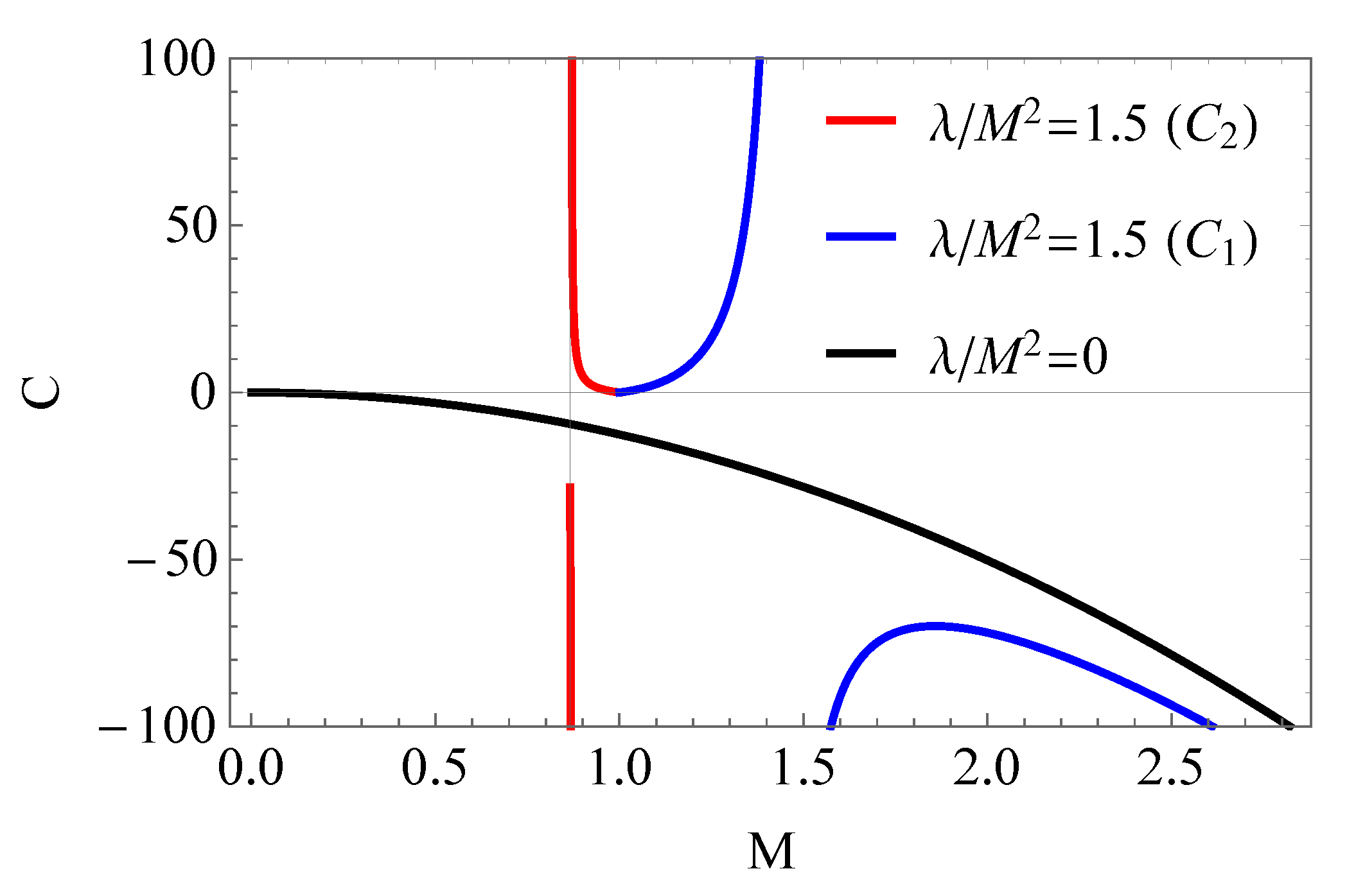
Let us write the corrected Hawking temperature using the metric (11) associated with the horizon $r_{h1}$ as

$$T_1=\frac{f^{\prime }\left(r\right)}{4\pi }{|}_{r=r_{h1}}=\frac{1}{4\pi R_H}\left(1-\frac{3}{2}\frac{\lambda }{R_H^2}\right).$$

(30)

It can be seen that for the critical value of the parameter

$$\begin{array}{c}\hfill {\lambda }_c=\frac{2R_H^2}{3}\end{array}$$

(31)

the Hawking temperature becomes zero, meaning that the black hole will stop radiating. In that case, small black holes do not disappear and remain as remnants. If now combine the last condition with Equation (22), we obtain

$$\begin{array}{c}\hfill {\lambda }_c=\frac{3}{2}{M}^2.\end{array}$$

(32)

This equation really shows that, at this critical value of $\lambda ={\lambda }_c$, a black hole with mass M will have zero Hawking temperature and, in general, the critical value of $\lambda$ depends on the black hole mass. We can see what exactly happens in Figure 4. If we fix for simplicity the black hole mass to unity [$M=1]$, in the interval $\lambda \in (1.5,2)$, the temperature $T_1$ becomes negative, which is not physically acceptable. However, as we will explain below, this is a consequence of the fact that, for $\lambda >{\lambda }_c$, the horizons switch places, and the outer horizon will be located at $r_{h2}$. Thus, in this region, Hawking temperature should be associated with the horizon $r_{h2}$, that is,

$$T_2=\frac{f^{\prime }\left(r\right)}{4\pi }{{|}_{r=r_{h2}}=\frac{1}{4\pi }\left(\frac{R_H}{r^2}-\frac{\lambda (4R_H^3-r^3)}{2r^5{R}_H}\right)|}_{r=r_{h2}}.$$

(33)

At the same critical value ${\lambda }_c=1.5$ where the black hole stops evaporating, the two horizons coincide, i.e., $r_{h1}=r_{h2}=1.5$ (see Figure 1, right panel). In the interval $\lambda \in (0,1.5)$, the outer horizon is $r_{h1}$, meaning that $r_{h1}>r_{h2}$, at the critical value ${\lambda }_c$ the two horizons coincide, while at the interval $\lambda \in (1.5,2)$, the outer horizon is now $r_{h2}$, meaning that $r_{h2}>r_{h1}$. Therefore, the Hawking temperature in the total interval is only the positive contribution obtained from the interval

$$T=\left\{\begin{array}{cc}{T}_1,\hfill & \lambda \in (0,1.5)\hfill \\ T_2,\hfill & \lambda \in (1.5,2)\hfill \end{array}\right.$$

(34)

We can see this fact also from the Figure 4. If we take $\lambda /M^2=1.5$, we see that, as the black hole mass decreases, the Hawking radiation increases and attains a maximum value when $(\partial T_{h1}/\partial r_{h1})=0$, we obtain the maximal value of the Hawking temperature at $M=1.443375673$. Now, if we further decrease the mass, we see that, at $M=1$, the Hawking temperature is exactly zero. On the other hand, if we have a black hole with mass in the range $M<1$, then there is a nonzero Hawking radiation coming from the horizon $r_{h2}$, with a Hawking temperature that increases and reaches a finite value at some minimal possible mass. We can obtain the minimal black hole mass using the condition $\lambda /M^2\le 2$, in our case [setting $\lambda =3/2$], we obtain $M_{min}=\sqrt{\lambda /2}=\sqrt{3}/2$. This can also be seen in Figure 2 (left panel) or in Figure 4 (right panel). Beyond this minimal mass, the black hole cannot exist, so we end up with some regular object or naked singularity.

To find the entropy of the black hole, we can use the first law of thermodynamics $\frac{\partial S}{\partial M}=\frac{1}{T}$ along with the expression for the temperature. Again, we will have two intervals for $\lambda$. The black hole horizon $r_{h1}$ contributes to the entropy in the domain $0<\lambda /M^2<1.5$. It is convenient to express the entropy in terms of the black hole horizon $r_{h1}=R_H$. For the entropy in this interval, we find

$$S=\int \frac{1}{T_1}\frac{\partial M}{\partial R_H}d{R}_H=\pi R_H^2+\pi \lambda ln\left(2R_H^2-3\lambda \right)+\mathcal{C},$$

(35)

where $\mathcal{C}$ is some constant of integration. Note that the black hole entropy consists of two terms; the first term is the standard Bekenstein–Hawking area law followed by the logarithmic string correction term. We can also express this entropy in terms of black hole mass by using Equation (19).

On the other hand, inside the interval $1.5<\lambda /M^2<2$, due to the contribution from the horizon $r_{h2}$, it is not possible to find an analytical closed form for the entropy. However, one can evaluate it numerically.

The thermodynamical stability of the black hole can be found by using the heat capacity $C_h$. The stability of the black hole is related to the sign of the heat capacity. In particular, when $C_h>0$, the black hole is stable, while, for $C_h<0$, the black hole is unstable. The heat capacity of the black hole is given by

$$C_h=\frac{\partial M_h}{\partial T_h}=\frac{\partial M_h}{\partial r_h}\frac{\partial r_h}{\partial T_h}.$$

(36)

In Figure 5, we plot the heat capacity of the black hole as a function of M for a fixed parameter $\lambda /M^2=1.5$. We can see that the total heat capacity $C_h$ of the black hole is obtained from the contribution of the horizon $r_{h1}$ noted as $C_1$ (blue line) in the interval $M\ge 1$, and the contribution of $C_2$ (red line) in the interval $M<1$. In particular, one can see that $C_1$ exhibits discontinuity and diverges at some critical points $r=r_c$, which can be linked to the second order phase transition. At the point $r=r_c$, there is a flip of sign in the heat capacity where the Hawking temperature attains a maximum value with $(\partial T_h/\partial r_h)=0$. In the interval $M<1$, we see that $C_2$ is positive and there is a discontinuity at the minimal mass $M_{min}=\sqrt{3}/2$. Beyond this point, the object is not a black hole; instead, it can be some regular object or a naked singularity. This means that the black hole is thermodynamically stable for $r_h<r_c$, whereas it is thermodynamically unstable for $r_h>r_c$. We also see that, in general, for large M, we have negative heat capacity $C_h<0$, hence the black hole is unstable. For a fixed value $\lambda /M^2=1.5$, the heat capacity is exactly zero at $M=1$, as expected, since the Hawking temperature becomes zero. It is also interesting to see that, for large values of M, the heat capacity gets closer and closer to the Schwarzschild black hole heat capacity, and it is also negative i.e., $C_h<0$. We note that there is no phase transition for the Schwarzschild black hole as can be seen from Figure 5 (black line).

3.3. Can $\lambda$ Be a Large Parameter?

As we mentioned earlier, the perturbative parameter $\lambda$ should be small in appropriate units. If that is true, then there is a great level of similarity between our 4D SCBH and the generalized uncertainty principle (GUP) corrected BH. This can be seen in the following. In the limit $\lambda \to 0$, we see from Equation (19) that the ADM mass gives $M_{ADM}=R_H$. This suggests that we can write

$$\begin{array}{c}\hfill R_H=2M_0,\end{array}$$

(37)

where $M_0$ can be interpreted as the bare mass of the black hole. The ADM mass can then be written as

$$\begin{array}{c}\hfill M_{ADM}=M_0\left(1+\frac{\lambda /4}{2M_0^2}\right).\end{array}$$

(38)

The second term on the right-hand side can be interpreted as the quantum mechanical hair due to the GUP. We start from the GUP equation in the form

$$\begin{array}{c}\hfill \Delta x=\frac{1}{\Delta p}+\frac{{\alpha }_{GUP}{l}_{\mathrm{Pl}}^2}{\hslash }\Delta p,\end{array}$$

(39)

where ${\alpha }_{GUP}$ is the GUP parameter, $l_{\mathrm{Pl}}=\sqrt{\hslash G/c^3}\sim {10}^{-33}$ cm is the Planck length. We set $\Delta x\to R$, $\Delta p\to cM$, where $M_0$ is the mass forming an event horizon if it falls within its own Schwarzschild radius $R_S=2G{M}_0/c^2$ (here, we have restored the constants c, ℏ and G). Using the $\beta$ (GUP corrected constant) formalism, it was shown in Ref. [23] that GUP has an important effect on the size of the black hole as follows:

$$\begin{array}{c}\hfill R_S^{\prime }=\frac{2G{M}_0}{c^2}\left(1+\frac{\beta }{2}{\left(\frac{M_{\mathrm{Pl}}}{M_0}\right)}^2\right)\end{array}$$

(40)

where $M_{\mathrm{Pl}}=\sqrt{\hslash c/G}\sim {10}^{-5}$ g. With appropriate units and the scaling

$$\beta \to \frac{\lambda }{4},$$

(41)

it can be easily seen that Equation (40) suggests a modified GUP ADM mass with $R_S^{\prime }=2M_{ADM}$. As a result, we can write

$$\begin{array}{c}\hfill M_{ADM}=\frac{G{M}_0}{c^2}\left(1+\frac{\beta }{2}{\left(\frac{M_{\mathrm{Pl}}}{M_0}\right)}^2\right).\end{array}$$

(42)

The last equation has been obtained in Refs. [23,24], but it coincides with our result for the ADM mass of the string corrected black hole given by Equation (38). This indicates that the string corrections given by (a small) $\lambda$ can be linked to the the GUP corrections $\beta$ of black holes.

However, $\lambda$ might not necessarily be a small parameter (in appropriate units). The rescaling given by Equation (9), ${\lambda }^{\prime }\to \lambda /(D-4)$, applied in Equations (6) and (7), is fine at the level of the solution for the metric (the terms $D-4$ cancel out), but it is not obviously justified at the level of the action in Equation (1), where singularity will appear in the limit of $D\to 4$. However, we can still analyze the metric given by the function in Equation (11), having in mind that we lost perturbative connection with the stringy action in Equation (1). Thus, $\lambda$ might not only encode small stringy corrections to the BH solutions (e.g., like GUP inspired corrections in Equation (38)), but also large corrections that might completely change physical interpretation of the solution (e.g., like for the critical value ${\lambda }_c$ in the previous section). As it was the case with 4D Gauss–Bonnet gravity, one expects a more general theory with a well defined action under the rescaling in (9). Such a regularized version of the action in Equation (1) is yet to be found, and is outside the scope of the present work. However, it is encouraging that solutions obtained by simple rescaling ${\alpha }^{\prime }\to {\alpha }^{\prime }/(D-4)$ in 4D Gauss–Bonnet gravity coincide with solutions following from a well defined regularized action, so we expect that something similar is happening here.

Incidentally, it was argued in [25] that the string tension necessarily becomes very low in Planck units when applied to an object like a black hole, which consists of many individual fundamental quanta. In that case, strings become elongated and “floppy" reaching the size of the black hole horizon, which gives the so-called fuzzball structure to the black hole. In the light of our analysis here, the metric given in terms of the ADM mass of the system (which is the total mass measured by a distant observer located far away from the black hole) is given by the function in Equation (23). This indicates that the string corrections might be hard to detect even if $\lambda$ is large (and thus tension is low), since the corrections decrease as $r^{-4}$.

4. The S2 Star Orbit

Let us first briefly review the basic calculations needed to obtain the orbit of S2 star assuming that the geometry is described by the 4D QCBH with the metric function (11). We start with the general D-dimensional spherically symmetric spacetime. Due to the spherical symmetry, one can assume that the orbit lies in the equatorial hyperplane:

$${\theta }_i(i=1,\dots ,D-3)=\pi /2,\mathrm{and}{\theta }_{D-2}=\varphi ,$$

(43)

Next, we use the coordinate transformation from spherical Schwarzschild coordinates to Cartesian coordinates given by

$$\begin{array}{ccc}\hfill x_1& =& rsin{\theta }_1\cdots sin{\theta }_{D-3}sin{\theta }_{D-2}sin{\theta }_{D-1}\hfill \\ \hfill x_2& =& rsin{\theta }_1\cdots sin{\theta }_{D-3}sin{\theta }_{D-2}cos{\theta }_{D-1}\hfill \\ \hfill x_3& =& rsin{\theta }_1\cdots sin{\theta }_{D-3}cos{\theta }_{D-2}\hfill \\ \hfill & ⋮& \\ \hfill x_{D-1}& =& rsin{\theta }_{1}cos{\theta }_2\hfill \\ \hfill x_D& =& rcos{\theta }_1.\hfill \end{array}$$

(44)

Using the last two equations, we obtain the polar coordinates

$$x_3=rcos\varphi ,x_1=rsin\varphi ,x_2=x_4=\cdots =0.$$

(45)

If we identify $x_3=x$, $x_1=y$, and $z=0$, we can obtain the equations of motion. We can work with this general D-dimensional case and treat the number of spacetime dimension as a parameter; however, we know that, at such large distances, the spacetime will be effectively 4D. For this reason, we shall simplify the problem and use our 4D SCBH. From the Lagrangian, it follows that

$$\begin{array}{ccc}\hfill 2\mathcal{L}& =& \left(1-\frac{R_H}{r}\right)\left(1-\frac{\lambda }{2R_{H}r}\frac{1-\frac{R_H^3}{r^3}}{1-\frac{R_H}{r}}\right){\dot{t}}^2\hfill \\ & -& \frac{{\dot{r}}^2}{\left(1-\frac{R_H}{r}\right)\left(1-\frac{\lambda }{2R_{H}r}\frac{1-\frac{R_H^3}{r^3}}{1-\frac{R_H}{r}}\right)}-r^2{\dot{\varphi }}^2\hfill \end{array}$$

(46)

From the spacetime symmetries, we have two constants of motion

$$\dot{t}=\frac{E}{\left(1-\frac{R_H}{r}\right)\left(1-\frac{\lambda }{2R_{H}r}\frac{1-\frac{R_H^3}{r^3}}{1-\frac{R_H}{r}}\right)},\dot{\varphi }=\frac{L}{r^2}$$

(47)

and

$$\ddot{r}={\displaystyle \frac{1}{2g_{rr}\left(r\right)}}\left[{\displaystyle \frac{d{g}_{00}\left(r\right)}{dr}}{\dot{t}}^2+{\displaystyle \frac{d{g}_{11}\left(r\right)}{dr}}{\dot{r}}^2+{\displaystyle \frac{d{g}_{\varphi \varphi }\left(r\right)}{dr}}{\dot{\varphi }}^2\right].$$

(48)

In terms of Cartesian coordinates, we denote the position of the real orbit as $(x,y,z)$, and velocity components $(v_x,v_y,v_z)$. In our present case, using the transformation from spherical Schwarzschild coordinates to Cartesian coordinates:

$$x=rcos\varphi ,y=rsin\varphi ,z=0,$$

(49)

we also find the corresponding three-velocities

$$v_x=v_{r}cos\varphi -r{v}_{\varphi }sin\varphi ,v_y=v_{r}sin\varphi +r{v}_{\varphi }cos\varphi .$$

(50)

We will use this to model the orbit of the S2 star in our geometry and compare it with the observational data to constrain two parameters—the mass M and parameter $\lambda$. To do so, we also need to find the apparent orbit on the plane of the sky by relating the coordinates $(\mathcal{X},\mathcal{Y},\mathcal{Z})$ to the real orbit given by $(x,y,z)$ as follows [26]:

$$\begin{array}{cc}\hfill \mathcal{X}& =xB+yG,\hfill \\ \hfill \mathcal{Y}& =xA+yF,\hfill \\ \hfill \mathcal{Z}& =xC+yF,\hfill \end{array}$$

(51)

The corresponding components of the apparent coordinate velocity are as follows [26]:

$$\begin{array}{cc}\hfill {\mathcal{V}}_X& =v_{x}B+v_{y}G,\hfill \\ \hfill {\mathcal{V}}_Y& =v_{x}A+v_{y}F,\hfill \\ \hfill {\mathcal{V}}_Z& =v_{x}C+v_{y}F,\hfill \end{array}$$

(52)

where [26]

$$\begin{array}{ccc}\hfill B& =& sin\Omega cos\omega +cos\Omega sin\omega cosi\hfill \end{array}$$

(53)

$$\begin{array}{ccc}\hfill G& =& -sin\Omega sin\omega +cos\Omega cos\omega cosi\hfill \end{array}$$

(54)

$$\begin{array}{ccc}\hfill A& =& cos\Omega cos\omega -sin\Omega sin\omega cosi\hfill \end{array}$$

(55)

$$\begin{array}{ccc}\hfill F& =& -cos\Omega sin\omega -sin\Omega cos\omega cosi\hfill \end{array}$$

(56)

$$\begin{array}{ccc}\hfill C& =& sin\omega sini\hfill \end{array}$$

(57)

$$\begin{array}{ccc}\hfill F& =& cos\omega sini,\hfill \end{array}$$

(58)

where $\omega$, i, and $\Omega$ are the argument of pericenter, the inclination between the real orbit and the observation plane, and the ascending node angle, respectively. Finding an analytical expression for $r\left(\varphi \right)$ is not possible; therefore, we use numerical integration of the equations of motion. To fit our 4D SCBH model, we have to solve the equations of motion numerically using the data presented in [26,27,28,29], and assuming the central mass object [30]. We use the Bayesian theorem according to which the observations O, and the vector containing the parameters of a model, say P, give the posterior probability density $\pi \left(P\right|O)$

$$\begin{array}{c}\hfill ln\pi \left(P\right|O)\propto ln\mathcal{L}(O\left|P\right)+ln\pi \left(P\right),\end{array}$$

(59)

where $\pi \left(P\right)$ is the prior probability density of the parameters. The likelihood function is given by

$$\begin{array}{ccc}\hfill ln\mathcal{L}\left(O\right|P)& =& -\frac{1}{2}\sum _{i=1}^N\left[\frac{{\left(X_{obs,i}-X_{mod,i}\right)}^2}{{\sigma }_{obs,i}^2}\right]\hfill \\ & -& \frac{1}{2}\sum _{i=1}^N\left[\frac{{\left(Y_{obs,i}-Y_{mod,i}\right)}^2}{{\sigma }_{obs,i}^2}\right],\hfill \end{array}$$

(60)

where the two observed and theoretical quantities are noted as $(X_{obs},Y_{obs})$, and $(X_{mod},Y_{mod})$, respectively. To find the best-fitting values, we use the Monte Carlo–Markov Chains analysis, with the uniform priors $\lambda /M^2\sim [0,2]$ along with $R_H/M\sim [0,3]$. In Figure 6 we give the orbit fit for our model. Our analyses show that the best-fitting value for the black hole parameter $R_H$ with $68\%$ confidence level is $R_H\sim 1.{74}_{-0.08}^{+0.12}\left[M\right]$ as shown in Figure 7. We also find the best fit value for the parameter $\lambda \sim 1.{10}_{-0.36}^{+0.21}\left[M^2\right]$ within a $68\%$ confidence level. In SI units, after reinstating G and c, for the string coupling parameter, we obtain the following value:

$$\begin{array}{c}\hfill \lambda \simeq 1.10\times {\left(\frac{GM}{c^2}\right)}^2\simeq 4\times {10}^{19}{\mathrm{m}}^2.\end{array}$$

(61)

As a comparison, using the precession of the S2 star in orbit around Sgr A${}^{*}$, the 4D Gauss–Bonnet coupling constant ${\alpha }_{GB}$ was constrained by an upper bound of ${\alpha }_{GB}\simeq {10}^{25}{\mathrm{m}}^2$ (see [16]). For the mass of the black hole, we find

$$M=\frac{R_H}{2}+\frac{\lambda }{4R_H}\simeq 1.{028}_{-0.086}^{+0.078}[4.07\times {10}^6{M}_{\odot }],$$

(62)

which is (within the errors) indistinguishable from the result in the Schwarzschild spacetime reported recently in Refs. [26,27,28,30]. We can also estimate the parameter $\xi =\lambda R_H^2/2\simeq 1.665\left[M^4\right]$. This indicates that the current precision is insufficient to distinguish the 4D SCBH spacetime from the Schwarzschild spacetime.

5. Einstein Rings in the Weak Field Regime

To study gravitational lensing, due to the spherical symmetry, we again consider the equatorial hyperplane. The photon trajectory (optical metric) is simply found by letting $\mathrm{d}{s}^2=0$, which gives

$$\begin{gathered} d{t}^2=\frac{d{r}^2}{{\left(1-\frac{R_H^{D-3}}{r^{D-3}}\right)}^2{\left(1-\frac{{\lambda }^{\prime }}{R_H^2}\frac{(D-3)(D-4)}{2}\frac{R_H^{D-3}}{r^{D-3}}\frac{1-\frac{R_H^{D-1}}{r^{D-1}}}{1-\frac{R_H^{D-3}}{r^{D-3}}}\right)}^2} \\ +\frac{r^{2}d{\varphi }^2}{\left(1-\frac{R_H^{D-3}}{r^{D-3}}\right)\left(1-\frac{{\lambda }^{\prime }}{R_H^2}\frac{(D-3)(D-4)}{2}\frac{R_H^{D-3}}{r^{D-3}}\frac{1-\frac{R_H^{D-1}}{r^{D-1}}}{1-\frac{R_H^{D-3}}{r^{D-3}}}\right)}. \end{gathered}$$

(63)

We will closely follow the method in [31] to compute the deflection angle of light. This geometric method is based on the application of the Gauss–Bonnet theorem (GBT) on the optical geometry. We consider a non-singular domain ${\mathcal{A}}_R$ with boundaries $\partial {\mathcal{A}}_R={\gamma }_{g^{\left(op\right)}}\cup C_R$, of an oriented two-dimensional surface S with the optical metric $g^{\left(op\right)}$. In terms of the Gaussian optical curvature (K) and the geodesic curvature ($\kappa$), we can write the GBT as follows [31]:

$$\underset{{\mathcal{A}}_R}{\int \int }K\mathrm{d}S+\underset{\partial {\mathcal{A}}_R}{\oint }\kappa \mathrm{d}t+\sum _k{\delta }_k=2\pi \chi \left({\mathcal{A}}_R\right).$$

(64)

in which $\mathrm{d}S$ is the optical surface element, ${\delta }_k$ gives the exterior angle at the $k^{th}$ vertex. We can relate the exterior angels with the interior angles (the jump angle at the source $\mathcal{S}$ and observer $\mathcal{O}$, respectively) using ${\theta }_{\mathcal{O}}=\pi -{\delta }_{\mathcal{O}}$ and ${\theta }_{\mathcal{S}}=\pi -{\delta }_{\mathcal{S}}$, which for a very large radial distance, i.e., $l\equiv R\to \infty$, satisfies the condition ${\theta }_{\mathcal{O}}+{\theta }_{\mathcal{S}}\to \pi$ (see [31]). According to this method, we need to choose the domain of integration to be outside of the light ray in the $(r,\varphi )$ optical plane. Moreover, this domain can be thought to have the topology of a disc having the Euler characteristic number $\chi \left({\mathcal{A}}_R\right)=1$. If we now introduce a smooth curve defined as $\gamma :=\left\{t\right\}\to {\mathcal{A}}_R$, we can find the geodesic curvature in terms of the following definition:

$$\kappa =g^{\left(op\right)}\left({\nabla }_{\dot{\gamma }}\dot{\gamma },\ddot{\gamma }\right),$$

(65)

along with the unit speed condition $g^{\left(op\right)}(\dot{\gamma },\dot{\gamma })=1$, and $\ddot{\gamma }$ being the unit acceleration vector. Note that, by definition, the geodesic curvature for the light ray (geodesics) ${\gamma }_{g^{\left(op\right)}}$ vanishes, i.e., $\kappa \left({\gamma }_{g^{\left(op\right)}}\right)=0$. One should only compute the contribution to the curve $C_R$. Thus, from the GBT, we find

$$\underset{R\to \infty }{lim}{\int }_0^{\pi +\widehat{\alpha }}{\left[\kappa \frac{dt}{d\varphi }\right]}_{C_R}d\varphi =\pi -\underset{R\to \infty }{lim}\underset{{\mathcal{A}}_R}{\int \int }K\mathrm{d}S.$$

(66)

The geodesic curvature for the curve $C_R$ located at a coordinate distance R from the coordinate system chosen at the black hole center can be calculated via the relation

$$\kappa \left(C_R\right)=\left|{\nabla }_{{\dot{C}}_R}{\dot{C}}_R\right|.$$

(67)

With the help of the unit speed condition, one can show that the asymptotically Euclidean condition is satisfied:

$$\begin{array}{c}\hfill \underset{R\to \infty }{lim}{\left[\kappa \frac{\mathrm{d}t}{\mathrm{d}\varphi }\right]}_{C_R}=1.\end{array}$$

(68)

From the GBT, it is not difficult to solve for the deflection angle, which gives

$$\widehat{\alpha }=-\underset{0}{\overset{\pi }{\int }}\underset{r=\frac{b}{sin\varphi }}{\overset{\infty }{\int }}K\mathrm{d}S.$$

(69)

Since we are interested in leading order terms, in the last equation for the integration domain, we have used an equation for the light ray as $r\left(\varphi \right)=b/sin\varphi$, where b is the impact parameter. The Gaussian optical curvature takes the form:

$$\begin{array}{ccc}\hfill K& \simeq & -\frac{(D-3)(D-2)}{2}\frac{R_H^{D-3}}{r^{D-1}}\hfill \\ & -& \frac{{(D-3)}^2(D-4)(D-2)R_H^{D-5}{\lambda }^{\prime }}{4r^{D-1}}\hfill \end{array}$$

(70)

Keeping only leading order terms, the deflection angle is

$$\begin{gathered} \widehat{\alpha }=-\underset{0}{\overset{\pi }{\int }}\underset{\frac{\mathsf{b}}{sin\varphi }}{\overset{\infty }{\int }}\left[-\frac{(D-3)(D-2)}{2}\frac{R_H^{D-3}}{r^{D-1}}\right]rdrd\varphi \\ -\underset{0}{\overset{\pi }{\int }}\underset{\frac{\mathsf{b}}{sin\varphi }}{\overset{\infty }{\int }}\left[-\frac{{(D-3)}^2(D-4)(D-2)R_H^{D-5}{\lambda }^{\prime }}{4r^{D-1}}\right]rdrd\varphi . \end{gathered}$$

(71)

Solving this integral, in the limit $b>>R_H$, and using the relation

$$\begin{array}{c}\hfill {\int }_0^{\pi }{sin}^n\varphi d\varphi =\frac{\sqrt{\pi }\Gamma \left(\frac{1+n}{n}\right)}{\Gamma \left(\frac{n+2}{2}\right)},\end{array}$$

(72)

to the leading order, we find

$$\begin{gathered} \widehat{\alpha }\simeq \frac{(D-3)(D-2)}{2}\frac{\sqrt{\pi }{R}_H^{D-3}\Gamma \left(\frac{D-2}{D-3}\right)b^{3D}}{\Gamma \left(\frac{D-1}{2}\right)} \\ +\frac{{(D-3)}^2(D-4)(D-2)}{4}\frac{\sqrt{\pi }{R}_H^{D-5}\Gamma \left(\frac{D-2}{D-3}\right)b^{3D}{\lambda }^{\prime }}{\Gamma \left(\frac{D-1}{2}\right)}. \end{gathered}$$

(73)

The leading order term agrees with a similar work in Ref. [32]. Finally, if we perform the rescaling ${\lambda }^{\prime }\to \lambda /(D-4)$ and $D=4$, we obtain

$$\widehat{\alpha }\simeq \frac{2R_H+\lambda /R_H}{b}.$$

(74)

From the last result, it appears that the deflection angle is affected by the string correction; however, a closer inspection allows for rewriting in terms of the black hole mass

$$\begin{array}{c}\hfill \widehat{\alpha }\simeq \frac{4\left(R_H/2+\lambda /4R_H\right)}{b}=\frac{4M}{b},\end{array}$$

(75)

which is identical to the Schwarzschild case. In fact, one can argue that the string correction term is proportional to $\delta {\widehat{\alpha }}_{string}\sim M^2\lambda /b^4$. Since $b>>M$, practically, this term is very very small. This means that we cannot distinguish the 4D SCBH from the Schwarzschild black hole using the leading term in the weak deflection angle. The small angles lens equation (in the weak deflection approximation) reads

$$\begin{array}{c}\hfill \beta =\theta -\frac{D_{LS}}{D_{OS}}\widehat{\alpha }.\end{array}$$

(76)

In the special situation $\beta =0$, when the source lies on (or passes through) the optical axis, an Einstein ring is formed. The weak deflection approximation, $\widehat{\alpha }\ll 1$ represents the angular radius of the Einstein ring given by

$$\begin{array}{c}\hfill {\theta }_E\simeq \frac{D_{LS}}{D_{OS}}\widehat{\alpha }\left(b\right).\end{array}$$

(77)

Here, we took into account that $D_{OS}=D_{OL}+D_{LS}$, when the angular source position is $\beta =0$. Keeping only the first order of the deflection angle and using the relation $b=D_{OL}sin\theta \simeq D_{OL}\theta$, the bending angle in the small angle approximation is

$$\begin{array}{c}\hfill {\theta }_E\simeq \sqrt{\frac{4M}{D_{OS}}\frac{D_{LS}}{D_{OL}}}.\end{array}$$

(78)

It follows that, using only the leading order terms in the weak gravity regime, one cannot distinguish the 4D SCBH geometry from the Schwarzschild by the means of Einstein rings either.

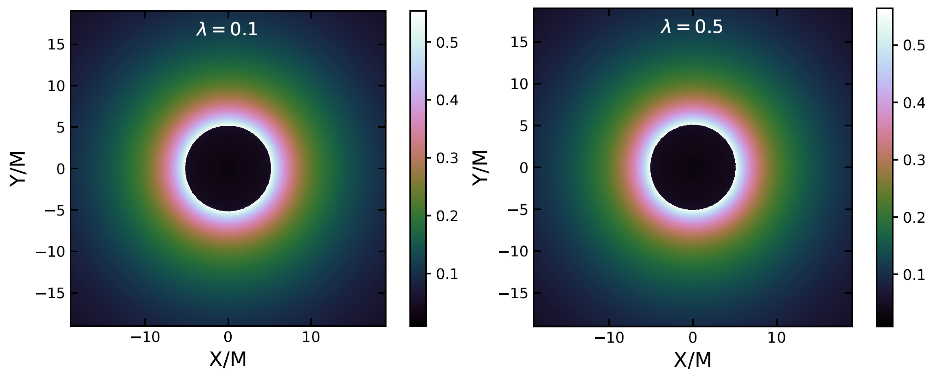
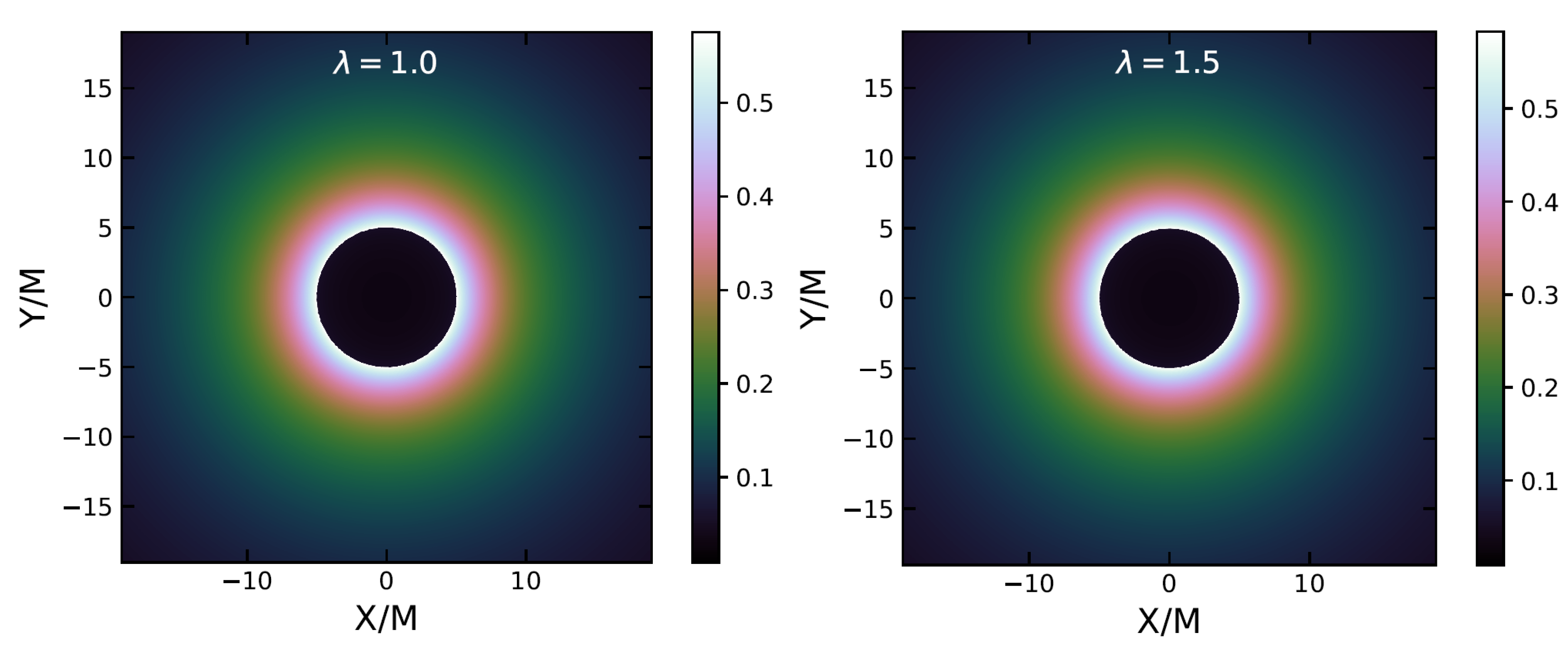
6. Shadow Images of a 4D SCBH

From the recent observations using the radio images, we know that there are supermassive black holes in galactic centers. In particular, the black-hole shadows have become a very useful tool to test not only the general relativity in the strong gravity regime but also to probe fundamental physics (see, for example, [33,34,35,36,37,38,39]). Obtaining a realistic image of the black hole is not an easy task. The main reason for this is the complicated surrounding matter near the black hole. In particular, the size, the shape, as well as the composition of the accretion disk, are all important. In addition, the geometry of magnetic field also influences the shadow [1,2]. In this work, we will consider a rather simple scenario of having an infalling gas model to obtain the black hole images [40,41,42,43,44]. For the four-velocity, we have [44]

$$\begin{array}{c}\hfill u_e^t=\frac{1}{f\left(r\right)},u_e^r=-\sqrt{\left(1-f\left(r\right)\right)},u_e^{\theta }=u_e^{\varphi }=0.\end{array}$$

(79)

On the other hand, we have a Hamilton–Jacobi equation

$$\frac{\partial S}{\partial \sigma }+H=0,$$

(80)

where S is the Jacobi action and $\sigma$ is an affine parameter along the geodesics. For the motion of photons in our 4D SCBH, we obtain

$$\frac{1}{2}\left[-\frac{p_t^2}{f\left(r\right)}+f\left(r\right)p_r^2+\frac{p_{\varphi }^2}{r^2}\right]=0,$$

(81)

where $p_t=-E$ and $p_{\varphi }=L$, are two constants of motions, namely the energy and the angular momentum of the photon, respectively. The unstable orbits are characterized by the conditions [45]

$$V_{\mathrm{eff}}\left(r\right){|}_{r=r_{ph}}=0,\frac{\partial V_{\mathrm{eff}}\left(r\right)}{\partial r}{|}_{r=r_{ph}}=0.$$

(82)

From the above equations, one can show [45]

$$\frac{dr}{d\varphi }=\pm r\sqrt{f\left(r\right)\left[\frac{r^{2}f\left(R\right)}{R^{2}f\left(r\right)}-1\right]}.$$

(83)

Let us consider a light ray sent from a static observer located at a position $r_0$ and transmitted at an angle $\vartheta$ with respect to the radial direction. We therefore have

$$cot\vartheta =\frac{\sqrt{g_{rr}}}{\sqrt{g_{\varphi \varphi }}}\frac{dr}{d\varphi }{|}_{r=r_0}.$$

(84)

Finally, the relation for shadow radius of the black hole as observed by a static observer at the position $r_0$ can be written as

$$R_{sh}=\underset{r_0\to \infty }{lim}R\sqrt{\frac{f\left(r_0\right)}{f\left(R\right)}}{|}_{R=r_{ph}}=\frac{r_{ph}}{\sqrt{f\left(r_{ph}\right)}},$$

(85)

where $r_{ph}$ represents the unstable photon orbit and $r_0$ is the position of the observer located at a far distance from the black hole. In Figure 8, we show how the shadow radius changes with the parameter $\lambda$. We observe that the shadow radius decreases initially in the interval $\lambda \in (0,1.5)$, it reaches the minimal value (or a reflecting point) at $\lambda /M^2=1.5$, and finally increases in the interval $\lambda \in (1.5,2)$. The presence of the reflecting point at ${\lambda }_c$ is explained by the fact that the shadow radius is proportional to the outer horizon. The minimal value of the shadow radius is obtained for $\lambda /M^2=1.5$, having $R_{sh}/M^2\simeq 5.0021$ with a photon sphere

$$r_{ph}=\frac{1}{2}+\frac{{(19+3\sqrt{33})}^{1/3}}{2}+\frac{2}{{(19+3\sqrt{33})}^{1/3}}\simeq 2.7589.$$

(86)

We use a numerical technique known as Backward Raytracing to find the shadow cast by the radiating flow. The total observed flux is given by

$$F_{obs}(X,Y)={\int }_{\gamma }{I}_{obs}({\nu }_{obs},X,Y)d{\nu }_{obs},$$

(87)

which can also be written as

$$F_{obs}(X,Y)={\int }_{\gamma }\int g^{4}j\left({\nu }_e\right)d{l}_{\mathrm{prop}}d{\nu }_e.$$

(88)

We shall assume that our emissivity is monochromatic with the radial profile given by

$$j\left({\nu }_e\right)\propto \frac{\delta ({\nu }_e-{\nu }_{*})}{r^2},$$

(89)

where $\delta$ is the Dirac delta function. If we use the condition $p_{\mu }{p}^{\mu }=0$, we can first obtain the relation between the radial and time component of the four momentum, and use the redshift function g given by

$$\begin{array}{c}\hfill g=\frac{k_{\alpha }{u}_o^{\alpha }}{k_{\beta }{u}_e^{\beta }}.\end{array}$$

(90)

We can then obtain the final expression for the observed flux as follows (for the details, see [44])

$$\begin{array}{c}\hfill F_{obs}(X,Y)\propto -{\int }_{\gamma }\frac{{\mathrm{g}}^3{k}_t}{r^2{k}^r}dr.\end{array}$$

(91)

In Figure 9, we have shown our results for the shadow images and the intensities of the 4D SCBH. In particular, we have shown four specific cases; the case with the $\lambda /M^2=\{0.1,0.5,1.0,1.5\}$, where the minimal shadow radius corresponds to the case $\lambda /M^2=1.5$. From the resulting images and their intensities, one can see that they look apparently the same in all cases. We can therefore conclude that the 4D SCBH is very difficult to distinguish from the Schwarzschild black hole. Notice also that, due to the fact that the deflection angle in leading order terms is the same in units of the black hole mass, this explains why the intensities of the electromagnetic radiation observed far away from the black hole will be almost the same as the Schwarzschild black hole. Such a small contribution is to be expected having in mind our metric (23) according to which the string corrections behave as the inverse of $r^4$.

7. Conclusions

In this paper, we performed a simple rescaling of the coupling parameter $\lambda$ in the D-dimensional Callan–Myers–Perry black hole to obtain a 4D black hole with string corrections. While we lose the direct connection to the original perturbative action, such a rescaling removes divergences at the level of equations of motion, which may give us a glimpse of what string corrections may look like in 4D.

Among the other things, we found that the black hole entropy acquires logarithmic corrections to the usual Bekenstein–Hawking entropy. We also found a critical value of the coupling parameter for which the Hawking temperature goes to zero. In contrast with the standard scenario where entropy goes to zero as the black hole evaporates completely, our black hole solution reaches a minimal entropy at some critical $\lambda$. For this value of $\lambda$, black holes leave stable remnants. While the black hole geometry still contains the central singularity even with stringy corrections, geodesics of the massive particles and light cannot reach it. We have also found a close connection between the string corrections and the GUP effects.

We have investigated the possibility of testing such a black hole geometry. We first constrained its parameters using the S2 star orbit at the galactic center. We calculated the light deflection angle and the Einstein rings to the leading order terms, as well as the corresponding shadow images using an infalling gas model. While the corrections depend on the string coupling parameter, in general, the magnitude of the change is too small to make a distinction from a Schwarzschild black hole. The maximal change occurs at $\lambda /M^2=1.5$, with $R_{sh}=5.0021\left[M\right]$. Compared to the Schwarzschild shadow radius ($3\sqrt{3}M$), this implies a change $\Delta R_{sh}\simeq 0.194\left[M\right]$. In terms of the angular radius, we can use ${\theta }_s=R_{sh}M/D$, for Sgr A${}^{*}$ black hole with mass $M\simeq 4.1\times {10}^6$M_⊙ and $D=8.3$ kpc, which implies the decrease on the angular size to be $\Delta {\theta }_s\simeq 1.40$$\mu$as. Although this is reasonable change, such an effect is out of reach using the current astronomical observations, but it remains an open question if such an effect can be observed in the near future.

References

1. Akiyama, K. et al. [Event Horizon Telescope Collaboration] First M87 Event Horizon Telescope Results. I. The Shadow of the Supermassive Black Hole. Astrophys. J. 2019, 875, L1. [Google Scholar] [CrossRef]
2. Akiyama, K. et al. [Event Horizon Telescope] First M87 Event Horizon Telescope Results. IV. Imaging the Central Supermassive Black Hole. Astrophys. J. 2019, 875, L4. [Google Scholar] [CrossRef]
3. Abbott, B.P. et al. [LIGO Scientific and Virgo Collaborations] Observation of Gravitational Waves from a Binary Black Hole Merger. Phys. Rev. Lett. 2016, 116, 061102. [Google Scholar] [CrossRef] [PubMed]
4. Callan, C.G.; Myers, R.C.; Perry, M.J. Black holes in string theory. Nucl. Phys. B 1989, 311, 673. [Google Scholar] [CrossRef]
5. Moura, F.; Rodrigues, J. Eikonal quasinormal modes and shadow of string-corrected d-dimensional black holes. Phys. Lett. B 2021, 819, 136407. [Google Scholar] [CrossRef]
6. Moura, F. String-corrected dilatonic black holes in d dimensions. Phys. Rev. D 2011, 83, 044002. [Google Scholar] [CrossRef] [Green Version]
7. Glavan, D.; Lin, C. Einstein-Gauss–Bonnet gravity in 4-dimensional space-time. Phys. Rev. Lett. 2020, 124, 081301. [Google Scholar] [CrossRef] [PubMed] [Green Version]
8. Konoplya, R.A.; Zhidenko, A. Black holes in the four-dimensional Einstein-Lovelock gravity. Phys. Rev. D 2020, 101, 084038. [Google Scholar] [CrossRef] [Green Version]
9. Jusufi, K. Nonlinear magnetically charged black holes in 4D Einstein-Gauss–Bonnet gravity. Ann. Phys. 2020, 421, 168285. [Google Scholar] [CrossRef]
10. Jusufi, K.; Banerjee, A.; Ghosh, S.G. Wormholes in 4D Einstein-Gauss–Bonnet Gravity. Eur. Phys. J. C 2020, 80, 698. [Google Scholar] [CrossRef]
11. Gürses, M.; Şişman, T.; Tekin, B. Is there a novel Einstein–Gauss–Bonnet theory in four dimensions? Eur. Phys. J. C 2020, 80, 647. [Google Scholar] [CrossRef]
12. Gurses, M.; Şişman, T.; Tekin, B. Comment on “Einstein-Gauss–Bonnet Gravity in 4-Dimensional Space-Time. Phys. Rev. Lett. 2020, 125, 149001. [Google Scholar] [CrossRef] [PubMed]
13. Ai, W. A note on the novel 4D Einstein-Gauss–Bonnet gravity. Commun. Theor. Phys. 2020, 72, 095402. [Google Scholar] [CrossRef]
14. Arrechea, J.; Delhom, A.; Jiménez-Cano, A. Comment on “Einstein-Gauss–Bonnet Gravity in Four-Dimensional Spacetime. Phys. Rev. Lett. 2020, 125, 149002. [Google Scholar] [CrossRef]
15. Fernandes, P.G.S. Charged Black Holes in AdS Spaces in 4D Einstein Gauss–Bonnet Gravity. Phys. Lett. B 2020, 805, 135468. [Google Scholar] [CrossRef]
16. Clifton, T.; Carrilho, P.; Fernandes, P.G.S.; Mulryne, D.J. Observational Constraints on the Regularized 4D Einstein-Gauss–Bonnet Theory of Gravity. Phys. Rev. D 2020, 102, 084005. [Google Scholar] [CrossRef]
17. Fernandes, P.G.S.; Carrilho, P.; Clifton, T.; Mulryne, D.J. Black Holes in the Scalar-Tensor Formulation of 4D Einstein-Gauss–Bonnet Gravity: Uniqueness of Solutions, and a New Candidate for Dark Matter. Phys. Rev. D 2021, 104, 044029. [Google Scholar] [CrossRef]
18. Fernandes, P.G.S.; Carrilho, P.; Clifton, T.; Mulryne, D.J. Derivation of Regularized Field Equations for the Einstein-Gauss–Bonnet Theory in Four Dimensions. Phys. Rev. D 2020, 102, 024025. [Google Scholar] [CrossRef]
19. Hennigar, R.A.; Kubizňák, D.; Mann, R.B.; Pollack, C. On taking the D → 4 limit of Gauss–Bonnet gravity: Theory and solutions. JHEP 2020, 7, 027. [Google Scholar] [CrossRef]
20. Tengherlini, F.R. Schwarzschild field in n dimensions and the dimensionality of space problem. Nuovo C. 1963, 27, 636. [Google Scholar] [CrossRef]
21. Shaikh, R. Shadows of rotating wormholes. Phys. Rev. D 2018, 98, 024044. [Google Scholar] [CrossRef] [Green Version]
22. Ali, A.F.; Khalil, M.M. Black Hole with Quantum Potential. Nucl. Phys. B 2016, 909, 173–185. [Google Scholar] [CrossRef] [Green Version]
23. Carr, B.J.; Mureika, J.; Nicolini, P. Sub-Planckian black holes and the Generalized Uncertainty Principle. JHEP 2015, 7, 052. [Google Scholar] [CrossRef] [Green Version]
24. Carr, B.; Mentzer, H.; Mureika, J.; Nicolini, P. Self-complete and GUP-Modified Charged and Spinning Black Holes. Eur. Phys. J. C 2020, 80, 1166. [Google Scholar] [CrossRef]
25. Mathur, S.D. The Fuzzball proposal for black holes: An Elementary review. Fortsch. Phys. 2005, 53, 793–827. [Google Scholar] [CrossRef] [Green Version]
26. Becerra-Vergara, E.A.; Argüelles, C.R.; Krut, A.; Rueda, J.A.; Ruffini, R. The geodesic motion of S2 and G2 as a test of the fermionic dark matter nature of our galactic core. Astron. Astrophys. 2020, 641, A34. [Google Scholar] [CrossRef]
27. Do, T.; Hees, A.; Ghez, A.; Martinez, G.D.; Chu, D.S.; Jia, S.; Sakai, S.; Lu, J.R.; Gautam, A.K.; O’neil, K.K.; et al. Relativistic redshift of the star S0-2 orbiting the Galactic Center supermassive black hole. Science 2019, 365, 664. [Google Scholar] [CrossRef] [Green Version]
28. Nampalliwar, S.; Kumar, S.; Jusufi, K.; Wu, Q.; Jamil, M.; Salucci, P. Modeling the Sgr A* Black Hole Immersed in a Dark Matter Spike. Astrophys. J. 2021, 916, 116. [Google Scholar] [CrossRef]
29. De Martino, I.; della Monica, R.; de Laurentis, M. f(R) gravity after the detection of the orbital precession of the S2 star around the Galactic Center massive black hole. Phys. Rev. D 2021, 104, L101502. [Google Scholar] [CrossRef]
30. Gillessen, S.; Plewa, P.M.; Eisenhauer, F.; Sari, R.E.; Waisberg, I.; Habibi, M.; Pfuhl, O.; George, E.; Dexter, J.; von Fellenberg, S.; et al. An Update on Monitoring Stellar Orbits in the Galactic Center. Astrophys. J. 2017, 837, 30. [Google Scholar] [CrossRef] [Green Version]
31. Gibbons, G.W.; Werner, M.C. Applications of the Gauss–Bonnet theorem to gravitational lensing. Class. Quantum Grav. 2008, 25, 235009. [Google Scholar] [CrossRef]
32. Belhaj, A.; Benali, M.; Balali, A.E.; Moumni, H.E.; Ennadifi, S.E. Deflection angle and shadow behaviors of quintessential black holes in arbitrary dimensions. Class. Quantum Grav. 2020, 37, 215004. [Google Scholar] [CrossRef]
33. Bambi, C.; Freese, K.; Vagnozzi, S.; Visinelli, L. Testing the rotational nature of the supermassive object M87* from the circularity and size of its first image. Phys. Rev. D 2019, 100, 044057. [Google Scholar] [CrossRef] [Green Version]
34. Vagnozzi, S.; Visinelli, L. Hunting for extra dimensions in the shadow of M87*. Phys. Rev. D 2019, 100, 024020. [Google Scholar] [CrossRef] [Green Version]
35. Atamurotov, F.; Jusufi, K.; Jamil, M.; Abdujabbarov, A.; Azreg-Aïnou, M. Axion-plasmon or magnetized plasma effect on an observable shadow and gravitational lensing of a Schwarzschild black hole. Phys. Rev. D 2021, 104, 064053. [Google Scholar] [CrossRef]
36. Papnoi, U.; Atamurotov, F. Rotating charged black hole in 4D Einstein–Gauss–Bonnet gravity: Photon motion and its shadow. Phys. Dark Univ. 2022, 35, 100916. [Google Scholar] [CrossRef]
37. Roy, R.; Vagnozzi, S.; Visinelli, L. Superradiance evolution of black hole shadows revisited. arXiv 2021, arXiv:2112.06932. [Google Scholar]
38. Yan, S.F.; Li, C.; Xue, L.; Ren, X.; Cai, Y.F.; Easson, D.A.; Yuan, Y.F.; Zhao, H. Testing the equivalence principle via the shadow of black holes. Phys. Rev. Res. 2020, 2, 023164. [Google Scholar] [CrossRef]
39. Qi, J.Z.; Zhang, X. A new cosmological probe using super-massive black hole shadows. Chin. Phys. C 2020, 44, 055101. [Google Scholar] [CrossRef]
40. Narayan, R.; Johnson, M.D.; Gammie, C.F. The Shadow of a Spherically Accreting Black Hole. Astrophys. J. 2019, 885, L33. [Google Scholar] [CrossRef] [Green Version]
41. Saurabh, K.; Jusufi, K. Imprints of dark matter on black hole shadows using spherical accretions. Eur. Phys. J. C 2021, 81, 490. [Google Scholar] [CrossRef]
42. Zeng, X.X.; Zhang, H.Q.; Zhang, H. Shadows and photon spheres with spherical accretions in the four-dimensional Gauss–Bonnet black hole. Eur. Phys. J. C 2020, 80, 872. [Google Scholar] [CrossRef]
43. Falcke, H.; Melia, F.; Agol, E. Viewing the shadow of the black hole at the galactic center. Astrophys. J. Lett. 2000, 528, L13. [Google Scholar] [CrossRef] [PubMed] [Green Version]
44. Bambi, C. Can the supermassive objects at the centers of galaxies be traversable wormholes? The first test of strong gravity for mm/sub-mm very long baseline interferometry facilities. Phys. Rev. D 2013, 87, 107501. [Google Scholar] [CrossRef] [Green Version]
45. Perlick, V.; Tsupko, O.Y.; Bisnovatyi-Kogan, G.S. Influence of a plasma on the shadow of a spherically symmetric black hole. Phys. Rev. D 2015, 92, 104031. [Google Scholar] [CrossRef] [Green Version]
Figure 1. Left panel: The plot shows the metric function for different values of λ . Right panel: The plot shows the two horizons by varying λ while keeping M = 1 . The two horizons coincide at λ c .
Universe 08 00194 g001
Figure 2. Left panel: Parametric plot between the mass of the black hole and the parameter λ . Right panel: Parametric plot between ξ and the parameter λ . We have set M = 1 .
Universe 08 00194 g002
Figure 3. Left panel: The velocity of light observed in a freely falling frame for light moving inward. Right panel: The velocity of light observed in a freely falling frame for light moving outward. We have set M = 1 .
Universe 08 00194 g003
Figure 4. Left panel:The plot showing Hawking temperature of the 4D SCBH as a function of the coupling parameter λ for a fixed mass of the black hole M = 1 . Right panel: The plot showing Hawking temperature of the 4D SCBH as a function of black hole mass for fixed values of the coupling parameter λ .
Universe 08 00194 g004
Figure 5. The plot showing the heat capacity of the black hole as a function of the black hole mass for a fixed values of the coupling parameter λ . For C h < 0 , the black hole is unstable.
Universe 08 00194 g005
Figure 6. The figure shows the orbit fit of the S2 star using the 4D SCBH geometry using the best fit parameters R H 1.74 [ M ] and λ 1.10 [ M 2 ] . The Sgr A * black hole is assumed to have a mass M = 4.07 × 10 6 M .
Universe 08 00194 g006
Figure 7. The figure shows the parametric plot of λ versus R H with 68% and 96% confidence contours.
Universe 08 00194 g007
Figure 8. Black hole shadow radius as a function of the parameter λ . We set the black hole mass to M = 1 .
Universe 08 00194 g008
Figure 9. Black hole shadow images and the intensities of the 4D SCBH using an infalling gas and radiation model using different values of λ . We set the black hole mass to M = 1 .
Universe 08 00194 g009aUniverse 08 00194 g009b
Publisher’s Note: MDPI stays neutral with regard to jurisdictional claims in published maps and institutional affiliations.