

Constraints on the Duration of Inflation from Entanglement Entropy Bounds

1
Higgs Centre for Theoretical Physics, School of Physics & Astronomy, University of Edinburgh, Edinburgh EH9 3FD, UK
2
Department of Physics, McGill University, Montreal, QC H3A 2T8, Canada
Universe 2022, 8(9), 438; https://doi.org/10.3390/universe8090438
Submission received: 12 June 2022
/
Revised: 12 August 2022
/
Accepted: 21 August 2022
/
Published: 24 August 2022
(This article belongs to the Special Issue Quantum Gravity Phenomenology II)
Abstract
:Using the fact that we only observe those modes that exit the Hubble horizon during inflation, one can calculate the entanglement entropy of such long-wavelength perturbations by tracing out the unobservable sub-Hubble fluctuations they are coupled with. On requiring that this perturbative entanglement entropy, which increases with time, obey the covariant entropy bound for an accelerating background, we find an upper bound on the duration of inflation. This presents a new perspective on the (meta-)stability of de Sitter spacetime and an associated lifetime for it.
Although cosmic inflation is widely regarded as the standard paradigm for the early universe, its embedding into a fundamental theory of quantum gravity (QG) remains an open question. Recently, there have been different arguments against long-lived accelerating spacetimes, especially in the context of string theory (ST) [1,2,3]. One such conjecture states that trans-Planckian modes should never cross the Hubble horizon during inflation, leading to an upper bound on the number of e-foldings [4]:
where H denotes the Hubble parameter during inflation. Although the physical motivation behind this conjecture—a trans-Planckian mode should never become part of late-time macroscopic inhomogeneities—has been heavily debated [5,6], it does find some connections to other aspects of the ST ‘swampland’ [7,8,9,10,11,12,13]. As a whole, there seem to be various obstructions to finding a quantum gravity completion for long-lived accelerating backgrounds. Although the specific technical difficulties have been realized in the context of ST, many of the arguments apply much more generally to any quantum gravity model. In particular, a corollary of this is that only extremely short-lived de Sitter (dS) spaces can arise in a UV-complete theory [2,4].
Indeed, it has been long argued that dS space is metastable from different points of view1. There are three time-scales often associated with the lifetime of dS—the scrambling time [21] corresponding to (1), the quantum breaking time , and the Poincaré recurrence time , where the Gibbons-Hawking entropy for dS is given by [22]. Clearly, (1) puts an upper bound on the number of e-foldings N that is much smaller than the other two time-scales, with drastic implications for inflation [23].
In this essay, we present a different argument for finding the maximum amount of e-foldings allowed for inflation and, therefore, set an upper bound on the lifetime of dS. Instead of invoking any QG reasoning, we employ a bottom-up argument by requiring that the entanglement entropy (EE) of scalar perturbations during inflation be bounded by the Gibbons–Hawking entropy. We note that the first arguments in favor of the so-called dS conjecture also followed from an application of the covariant entropy bound (CEB) and the distance conjecture [2]. However, that derivation was (i) intimately tied to details of ST and (ii) valid only in asymptotic regions of moduli space. Here, we circumvent both these obstructions.
Discussions of EE have become ubiquitous in the context of gravity. However, in most cases, one considers the EE between different geometric regions of space—in the context of black holes [24], Minkowski [25], or dS space [26]. Moreover, the EE of cosmological backgrounds have sometimes been carried out using holographic methods [27,28]. Nevertheless, it is not necessary to define a subsystem, which is separated out in the position space domain, e.g., demarcation by a black hole horizon. In cosmology, it is more instructive to consider EE between different bands in momentum space, since it is the correlation functions of the momentum modes of cosmological perturbations, which are generally probed. For momentum space, the vacuum of the free field theory is factorized, and any EE come from the interactions that lead to mode coupling.
One can calculate the perturbative EE in momentum space for a scalar in flat spacetime as outlined, for example, in [29]. The full Hilbert space can be partitioned into two parts separated by some fiducial momentum scale such that . The Hamiltonian of the system is decomposed as
where are the free Hamiltonians of the respective subsystems, and the interacting Hamiltonian has a coupling parameter . The ground state is the product of the individual harmonic vacua of and , i.e., . The energy eigenbasis of and are denoted by and , respectively, while the corresponding energy eigenvalues are and . The (perturbative) interacting vacuum can be written as (up to normalization)
where the matrix elements and are calculated using standard perturbation theory. The reduced density matrix corresponding to subsystem is obtained by tracing out the modes. From that, one can extract the leading order contribution to the (von Neumann) EE:
where it is understood that at least one momentum in the matrix element is below , and at least one momentum is above.
The main calculation of [30] was to extend this result to an inflating background, which we now present. Considering the density perturbations in the comoving gauge
where a and are the usual symbols for the scale factor and the (first) slow-roll parameter for a quasi-dS expansion written as functions of the conformal time . The quadratic action for , in terms of momentum modes, describes a collection of harmonic oscillators with a time-dependent mass term. This implies a difference between the quasi-dS geometry and Minkowski background [30]—the sub-Hubble modes () are in their quantum (Bunch-Davies) vacuum, while the super-Hubble ones () are in a (two-mode) squeezed state [31]. Thus, the ground state factorizes as
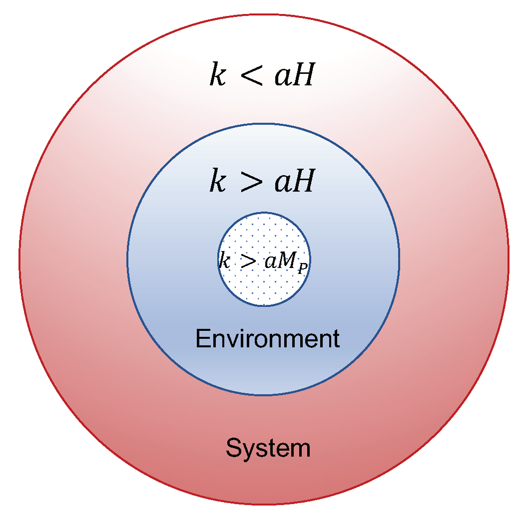
Since the modes which exit the horizon during inflation can only be later observed, we consider the super-Hubble modes as our system (), while the sub-Hubble ones are the environment () (Figure 1). (The dynamics of this system were studied in [32].) Finally, the nonlinearity of GR also provides us with an interaction term which couples the sub- and super-Hubble modes; thus, this interaction is universal and can never be turned off.
Mathematically, this translates into having a Hilbert space: where , and similarly for the sub-Hubble modes. The full Hamiltonian is given by , where
is the leading order cubic non-Gaussian term (since “freezes” outside the horizon) out of all the available interactions [33]. We now need to apply time-dependent perturbation theory to calculate the matrix elements since is time dependent. Moreover, there is no well-defined notion of energy for the squeezed state, but we only need energy differences in (4). This is a rather important point which deserves further explanation. Definitions of entanglement entropy in flat space can heavily depend on notions of energy which, in turn, is dependent on the Hamiltonian (and the corresponding vacuum) for the system. It is well known that there are ambiguities in defining the vacuum (or initial) state for inflation. In this particular case, we assume that all the scalar quantum fluctuations started out in their Bunch–Davies vacuum, while the modes that crossed the Hubble horizon correspond to the squeezed state. Although there is no good notion of energy for the squeezed vacuum, we can nevertheless define excited states (as N-particle states by acting with the relevant number of creation operators over the squeezed vacuum). Furthermore, we only need the difference in the energy between these excited states and the squeezed vacuum, which can be expressed in terms of the physical momenta of the ladder operators. This is why we are able to generalize the standard definition of EE in flat space to that for inflation [30].
Using these inputs, one can carefully evaluate (4) for inflationary perturbations [30], resulting in the EE (per unit physical volume):
where is the scale factor at the (end) beginning of inflation. In this calculation, it was assumed that there were no super-Hubble modes at the beginning of inflation, and both remain constant. It was shown that the dominant contribution comes from the squeezed configuration, and in the large squeezing limit, we present the leading order estimate omitting some factors as well as small logarithmic corrections [30].
Firstly, we note that the resulting EE between the sub- and super-Hubble modes is sensitive to the UV-cutoff , as expected. Note that this is not an artificial cutoff introduced in the system, but rather one should take the view that the Planck mass is an energy scale beyond which we should not expect standard cosmological perturbation theory on a classical inflationary background to be valid any longer. However, what is remarkable about this result is that the EE increases secularly with time, as signified by the term. The intuitive reason for this is that the dimension of increases with time as modes get stretched outside the horizon. It is not surprising that the EE is increasing with time, as it does for many systems with dynamical backgrounds. This is indeed what we would expect to happen for any cosmological (expanding) spacetimes. However, what is remarkable for inflation is that the rate of increase is very high due to the exponential expansion of the background. Thus, although we have calculated the EE as a perturbative quantity here, it will necessarily become very "large” over time.
Let us quantify the last statement made above. We used standard perturbation theory to calculate the first-order matrix element, which has given us the leading order EE for the density fluctuations during inflation. Given that this is a perturbative calculation, it is automatically a small quantity suppressed by factors of the interaction parameter of the cubic nonlinear term. However, we find that given enough time, this perturbative EE will soon become quite large and can overcome any entropy bound. To give us an idea of this, we can consider different entropy bounds. It was shown in [30] that if we demand that the EE remains subdominant to the thermal entropy, then we end up with a bound for the duration of inflation that is very close to the one derived from the TCC.
In this work, we want to use the background Gibbons–Hawking entropy as the upper bound for it. The main idea is that the growth of entropy often leads to deep puzzles in theoretical physics, and we wish to make our most crucial observation in this context. We require that the total EE obeys the CEB [34], i.e., the EE in a Hubble patch can, at most, saturate the entropy corresponding to the apparent horizon (). The reader might be a bit confused here as to why we are comparing our momentum space EE with the Gibbons–Hawking entropy, which is something calculated in position space. However, we are not actually claiming that the momentum space EE calculated here must satisfy the CEB. In fact, the CEB is a bound for real space entropy for a causal patch, whereas we are calculating a momentum space EE. Therefore, in order to be more precise, one would have to take our momentum space result and try to "Fourier transform” it to real space in order to obtain a strict bound from the CEB.
However, our goal is somewhat different here. We are merely interested in generalizing the results of [30] by using the CEB as a measure to point out how rapidly the EE is increasing, and even a perturbative quantity like itself can overcome the CEB within a few e-foldings. In fact, our main argument is that any bound on the EE—whether it is the thermal entropy during reheating or the CEB—will soon be saturated. Even more interestingly, the quantitative measure of how soon the EE saturates any such entropy bound is seemingly always related to the scrambling time of dS, as shown below.
More explicitly, requiring that the EE saturates the CEB (where the total for inflation), we find the relation:
With the observed power spectrum , one finds , and therefore,
This bound on the number of e-foldings is very similar to the one in (1), without requiring any QG input, and it predicts an upper limit on the lifetime of dS given by
closely related to the scrambling time up to small factors. Our result has far-reaching implications both for the UV-completions of dS space as well as the phenomenological predictions of inflation2. Interestingly, a very similar bound on the duration of inflation was derived from measures of complexity and chaos for inflationary perturbations [35], adding more evidence that the EE grows to such values on scrambling times that the standard EFT of inflation fails on these scales.
An immediate question is the implication for our bound on specific models of inflation. What is clear for from (11) is that the lifetime is larger for low-scale models of inflation. In other words, models with lower energy scales of inflation (given by the Hubble scale H) will be preferred according to this. Apart from the fact that such models will have a larger lifetime according to (10), they are also the ones which require a lower number of e-folds in order to solve the horizon and flatness problems. Therefore, GUT-scale models (which generically produce a large tensor-to-scalar ratio) are disfavored by our bounds. This, by itself, is not a large problem for inflation since there are plenty of small-field models (which would be the ones obeying the above condition if we allow for single-field models only). However, it is known that these models lose the preferred "attractor” feature of inflation [23,36], since it is clear that only small-field models are preferred by (10), which rules out polynomial potentials (such as the quadratic one) and only allows for hilltoplike potentials (which have a very small tensor-to-scalar ratio). As an example, for typical GUT-scale models , the number of e-foldings allowed would be . This is, of course, completely incompatible with the required number of e-foldings to explain, for example, the horizon problem. This gives us an insight into why low-scale models of inflation are the only ones allowed by this bound.
To summarize, for a dS geometry, an observer has access to only part of the entire spacetime. In particular for inflation, tracing out the unobservable sub-Hubble modes leads to a non-zero EE for the curvature perturbations that increases with time. However, since the EE can, at best, saturate the CEB, this puts an upper limit on the duration of inflation. Our calculation provides an universal limit since we take the simplest case of a minimally-coupled scalar field—any additional fields or extra-couplings (which give rise to stronger non-Gaussian) would only enhance the EE and strengthen our result. We emphasize that our bound does not arise from demanding a finite-dimensional Hilbert space for dS [37] or that we live in an asymptotically dS universe [38]. Finally, note that EE for other early-universe scenarios do not produce such bounds on the lifetime [39].
Funding
S.B. is supported in part by the Higgs Fellowship.
Institutional Review Board Statement
Not applicable.
Informed Consent Statement
Not applicable.
Data Availability Statement
Not applicable.
Acknowledgments
I am grateful to Robert Brandenberger for multiple discussions. I am also thankful to an anonymous referee for suggestions that led to improving the draft.
Conflicts of Interest
The author declares no conflict of interest.
| 1 | |
| 2 | A direct evaluation of EE in momentum space for a scalar field on pure dS, as well as a more sophisticated calculation of the inflationary system allowing for a slowly varying H and , shall be carried out in the future. |
References
- Palti, E. The swampland: Introduction and review. Fortschritte der Physik 2019, 67, 1900037. [Google Scholar] [CrossRef] [Green Version]
- Ooguri, H.; Palti, E.; Shiu, G.; Vafa, C. Distance and de Sitter Conjectures on the Swampland. Phys. Lett. B 2019, 788, 180–184. [Google Scholar] [CrossRef]
- Garg, S.K.; Krishnan, C. Bounds on slow roll and the de Sitter swampland. J. High Energy Phys. 2019, 2019, 75. [Google Scholar] [CrossRef] [Green Version]
- Bedroya, A.; Vafa, C. Trans-Planckian censorship and the swampland. J. High Energy Phys. 2020, 2020, 123. [Google Scholar] [CrossRef]
- Burgess, C.P.; de Alwis, S.P.; Quevedo, F. Cosmological trans-Planckian conjectures are not effective. J. Cosmol. Astropart. Phys. 2021, 2021, 37. [Google Scholar] [CrossRef]
- Dvali, G.; Kehagias, A.; Riotto, A. Inflation and decoupling. arXiv 2020, arXiv:2005.05146. [Google Scholar]
- Bedroya, A. de Sitter Complementarity, TCC, and the Swampland. arXiv 2020, arXiv:2010.09760. [Google Scholar] [CrossRef]
- Rudelius, T. Dimensional reduction and (Anti) de Sitter bounds. J. High Energy Phys. 2021, 2021, 41. [Google Scholar] [CrossRef]
- Andriot, D. Tachyonic de Sitter solutions of 10d type II supergravities. Fortschritte der Physik 2021, 69, 2100063. [Google Scholar] [CrossRef]
- Andriot, D.; Cribiori, N.; Erkinger, D. The web of swampland conjectures and the TCC bound. J. High Energy Phys. 2020, 2020, 162. [Google Scholar] [CrossRef]
- Berera, A.; Brahma, S.; Calderón, J.R. Role of trans-Planckian modes in cosmology. J. High Energy Phys. 2020, 2020, 71. [Google Scholar] [CrossRef]
- Brahma, S. Trans-Planckian censorship conjecture from the swampland distance conjecture. Phys. Rev. D 2020, 101, 046013. [Google Scholar] [CrossRef] [Green Version]
- Aalsma, L.; Shiu, G. Chaos and complementarity in de Sitter space. J. High Energy Phys. 2020, 2020, 152. [Google Scholar] [CrossRef]
- Goheer, N.; Kleban, M.; Susskind, L. The trouble with de Sitter space. J. High Energy Phys. 2003, 2003, 056. [Google Scholar] [CrossRef]
- Arkani-Hamed, N.; Dubovsky, S.; Nicolis, A.; Trincherini, E.; Villadoro, G. A measure of de Sitter entropy and eternal inflation. J. High Energy Phys. 2007, 2007, 55. [Google Scholar] [CrossRef] [Green Version]
- Kachru, S.; Kallosh, R.; Linde, A.; Trivedi, S.P. De Sitter vacua in string theory. Phys. Rev. D 2003, 68, 046005. [Google Scholar] [CrossRef] [Green Version]
- Dubovsky, S.; Senatore, L.; Villadoro, G. The volume of the universe after inflation and de Sitter entropy. J. High Energy Phys. 2009, 2009, 118. [Google Scholar] [CrossRef] [Green Version]
- Dvali, G.; Gómez, C.; Zell, S. Quantum break-time of de Sitter. J. Cosmol. Astropart. Phys. 2017, 2017, 028. [Google Scholar] [CrossRef] [Green Version]
- Brahma, S.; Dasgupta, K.; Tatar, R. de Sitter space as a Glauber-Sudarshan state. J. High Energy Phys. 2021, 2021, 104. [Google Scholar] [CrossRef]
- Brahma, S.; Dasgupta, K.; Tatar, R. Four-dimensional de Sitter space is a Glauber-Sudarshan state in string theory. J. High Energy Phys. 2021, 2021, 114. [Google Scholar] [CrossRef]
- Susskind, L. Addendum to fast scramblers. arXiv 2011, arXiv:1101.6048. [Google Scholar]
- Gibbons, G.W.; Hawking, S.W. Cosmological event horizons, thermodynamics, and particle creation. In Euclidean Quantum Gravity; World Scientific: Singapore, 1993; pp. 281–294. [Google Scholar]
- Bedroya, A.; Brandenberger, R.; Loverde, M.; Vafa, C. Trans-Planckian censorship and inflationary cosmology. Phys. Rev. D 2020, 101, 103502. [Google Scholar] [CrossRef]
- Solodukhin, S.N. Entanglement entropy of black holes. Living Rev. Relativ. 2011, 14, 8. [Google Scholar] [CrossRef] [PubMed] [Green Version]
- Casini, H.; Huerta, M. Entanglement entropy in free quantum field theory. J. Phys. A Math. Theor. 2009, 42, 504007. [Google Scholar] [CrossRef]
- Maldacena, J.; Pimentel, G.L. Entanglement entropy in de Sitter space. J. High Energy Phys. 2013, 2013, 38. [Google Scholar] [CrossRef] [Green Version]
- Giataganas, D.; Tetradis, N. Entanglement entropy in FRW backgrounds. Phys. Lett. B 2021, 820, 136493. [Google Scholar] [CrossRef]
- Giantsos, V.; Tetradis, N. Entanglement entropy in a four-dimensional cosmological background. arXiv 2022, arXiv:2203.06699. [Google Scholar] [CrossRef]
- Balasubramanian, V.; McDermott, M.B.; Van Raamsdonk, M. Momentum-space entanglement and renormalization in quantum field theory. Phys. Rev. D 2012, 86, 045014. [Google Scholar] [CrossRef] [Green Version]
- Brahma, S.; Alaryani, O.; Brandenberger, R. Entanglement entropy of cosmological perturbations. Phys. Rev. D 2020, 102, 043529. [Google Scholar] [CrossRef]
- Albrecht, A.; Ferreira, P.; Joyce, M.; Prokopec, T. Inflation and squeezed quantum states. Phys. Rev. D 1994, 50, 4807. [Google Scholar] [CrossRef] [Green Version]
- Brahma, S.; Berera, A.; Calderón-Figueroa, J. Universal signature of quantum entanglement across cosmological distances. arXiv 2021, arXiv:2107.06910. [Google Scholar]
- Maldacena, J. Non-Gaussian features of primordial fluctuations in single field inflationary models. J. High Energy Phys. 2003, 2003, 13. [Google Scholar] [CrossRef]
- Bousso, R. A covariant entropy conjecture. J. High Energy Phys. 1999, 1999, 4. [Google Scholar] [CrossRef] [Green Version]
- Bhattacharyya, A.; Das, S.; Haque, S.S.; Underwood, B. Rise of cosmological complexity: Saturation of growth and chaos. Phys. Rev. Res. 2020, 2, 033273. [Google Scholar] [CrossRef]
- Brandenberger, R. Initial conditions for inflation—A short review. Int. J. Mod. Phys. D 2017, 26, 1740002. [Google Scholar] [CrossRef] [Green Version]
- Banks, T. Cosmological breaking of supersymmetry? Int. J. Mod. Phys. A 2001, 16, 910–921. [Google Scholar] [CrossRef]
- Banks, T.; Fischler, W. An upper bound on the number of e-foldings. arXiv 2003, arXiv:astro-ph/0307459. [Google Scholar]
- Brahma, S.; Brandenberger, R.; Wang, Z. Entanglement entropy of cosmological perturbations for S-brane Ekpyrosis. J. Cosmol. Astropart. Phys. 2021, 2021, 94. [Google Scholar] [CrossRef]
Figure 1.
Schematic illustration of the system and environment modes for this setup. Gravity plays the role of providing a natural scale—the comoving Hubble horizon—which demarcates “long” and “short” degrees of freedom (dofs). We impose the Planck mass as the natural cutoff for the UV-modes and assume that these can be properly accounted for within some QG theory.
Publisher’s Note: MDPI stays neutral with regard to jurisdictional claims in published maps and institutional affiliations. |
© 2022 by the author. Licensee MDPI, Basel, Switzerland. This article is an open access article distributed under the terms and conditions of the Creative Commons Attribution (CC BY) license (https://creativecommons.org/licenses/by/4.0/).
Share and Cite
MDPI and ACS Style
Brahma, S. Constraints on the Duration of Inflation from Entanglement Entropy Bounds. Universe 2022, 8, 438. https://doi.org/10.3390/universe8090438
AMA Style
Brahma S. Constraints on the Duration of Inflation from Entanglement Entropy Bounds. Universe. 2022; 8(9):438. https://doi.org/10.3390/universe8090438
Chicago/Turabian StyleBrahma, Suddhasattwa. 2022. "Constraints on the Duration of Inflation from Entanglement Entropy Bounds" Universe 8, no. 9: 438. https://doi.org/10.3390/universe8090438
Note that from the first issue of 2016, this journal uses article numbers instead of page numbers. See further details here.