1. Introduction
In recent years, the study of the terrestrial ionosphere in relation to various extreme phenomena has become a very interesting topic. Using various observation techniques, many scientists around the world have made significant progress in studying the imprints of extreme phenomena in the ionosphere [
1,
2]. As a result, the ionosphere is recognized as a useful “tool” for studying the disturbances caused by such phenomena. Modern communication systems, including satellite and navigation systems, as well as various radio signals, traverse the atmosphere and lower ionosphere. It is worth noting that these signals may encounter disturbances during periods of solar perturbations. X-ray solar flares can be classified based on their influence on VLF wave propagation via the Earth–ionosphere waveguide [
3]. The significance of modeling the lower ionosphere cannot be overstated in relation to diverse technological, research, and industrial fields [
4].
VLF ionospheric data modelling, like any other type of modelling, involves a preliminary data pre-processing phase. During this phase, data filtering and domain-specific transformations are usually applied, along with the elimination of erroneous data points. In the context of VLF ionospheric amplitude analysis, the methodology bears resemblance to the aforementioned approach. However, it diverges in the sense that the elimination of two distinct categories of erroneous data points is required. The first category pertains to instrumentation errors, wherein the VLF receiver produces flawed measurements. The second category involves the researcher’s decision to either exclude or annotate the data points affected by the solar flare influences on the VLF data. The process of manually eliminating and/or annotating erroneous data in VLF data analysis is subject to an additional consideration, namely, the high measurement resolution, i.e., measurements taken at one minute intervals. The volume of data gathered during a given period of investigation can be overwhelming, requiring significant time and effort to manually sift through it and exclude. Consequently, the automation of this process is considered to be highly advantageous.
One crucial element in the field of space weather physics pertains to the interrelationship among solar flare (SF) occurrences, the ionospheric reaction to such events, and Coronal Mass Ejections (CME) [
2]. The importance of SF occurrences, including those classified as lower M-class rather than X-class, holds considerable significance and is currently a research focus. SF events classified as M-class exhibit a lower correlation with CMEs compared to X-class flares; however, a subset of M-class flares has been found to be associated with faster CMEs [
5], which aligns with the concept known as Big Flare Syndrome [
5,
6]. Moreover, there exists a significant correlation between X-class SFs of great intensity and CMEs, which have been observed to induce disruptions to satellite and navigation systems [
7].
The current research in the fields of SFs, CMEs, and the ionosphere is focused on the application of machine learning (ML) techniques. Classification methods have been employed in the classification of lighting waveforms [
8], as well as in the classification of radar returns [
9,
10,
11,
12,
13] and auroral image classification [
14,
15]. Similar to the pre-processing phase of VLF data analysis, manual radar return classification entails human intervention and is a labor-intensive procedure [
9]. The resemblance between the two aforementioned processes underscores the justification for employing ML classification techniques in order to automatically eliminate and/or classify erroneous ionospheric VLF data.
In order to streamline the manual exclusion or labeling of inaccurate ionospheric VLF data, the application of ML classification techniques has been considered. The aim of this study was to employ pre-existing ionospheric VLF amplitude data (Worldwide Archive Of Low-Frequency Data And Observations—WALDO,
https://waldo.world/, accessed on 24 March 2023) that have been previously utilized in research, as well as soft range X-ray irradiance data (Geostationary Operational Environmental Satellite—GOES,
https://www.ncei.noaa.gov/, accessed on 24 March 2023), with the purpose of investigating the feasibility of automatically labeling erroneous data and the effects of increased solar flare activity on measured VLF data. The task involved the utilization of the Random Forest (RF) method for ML classification. The data used for this task consisted of a total of 19 transmitter–receiver (T-R) pairs which are situated in North America. The data spanned the time period between September 2011 and October 2011, during which, solar flare activity was observed. In addition, in the manuscript, we discuss how the presented research serves as a potential method for the automated labeling of data in various fields of space science. The used datasets, results, and a post-processing workflow can be found on Zenodo:
https://zenodo.org/record/8220971, accessed on 7 August 2023 (
Supplementary Materials).
2. Materials and Methods
The present study made use of data obtained in 2011, specifically data gathered during solar flare events that took place in September (ranging from C2.5 to X2.1) and October (ranging from C5.5 to M1.5). The data employed in this study had already undergone a process of “labeling”, wherein erroneous data points were previously excluded (
Figure 1). This circumstance presented a distinctive opportunity to utilize the dataset for the purpose of training a ML model, which, in turn, could potentially automate the process of labeling in subsequent instances.
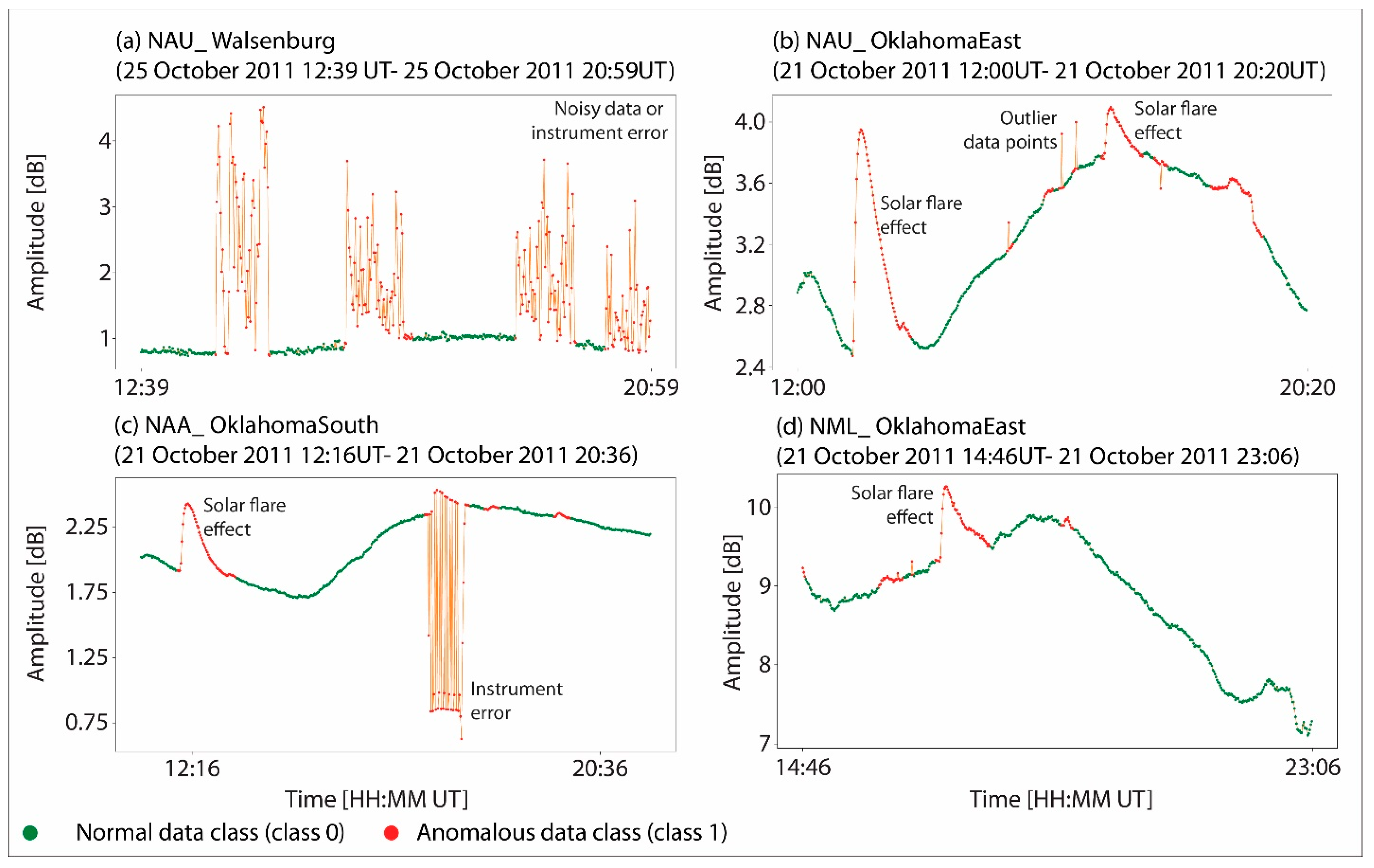
Figure 1 illustrates four instances in which a researcher was required to manually exclude erroneous data points from the dataset in preparation for a subsequent analysis.
Figure 1a illustrates the impact of noisy data or errors in instrumentation on VLF data. Conversely,
Figure 1b demonstrates the effects of SFs on VLF data, including the presence of outlier data points (single data points that significantly deviate from the rest of the measured data points).
Figure 1c,d exhibit a confluence of SF impacts, anomalous data points, and instrumentation errors. The aforementioned instances have a direct impact on the processing time required, i.e., the “data cleaning”. This is particularly significant due to the high measurement rate and the time spans of VLF data. Consequently, this may result in large datasets and necessitate a substantial amount of time for the manual exclusion of such data.
The dataset employed in this study comprised five VLF transmitters, namely NPM, NLK, NML, NAA, and NAU, along with four VLF receivers, specifically Walsenburg, Oklahoma South, Oklahoma East, and Sheridan (
Figure 2). There was a total of 19 T-R pairs.
In standard ML workflows, a crucial step involves the pre-processing of data (
Figure 3). During this phase, the data are transformed in order to meet to the requirements of the ML methods, i.e., dataset formats. Additionally, features are extracted, which will serve the purpose of revealing important patterns and characteristics within the dataset. Furthermore, the complete dataset is divided into separate training and testing datasets. In cases where the classes within the training dataset are imbalanced, it is common practice to balance them. This balancing process enhances the evaluation metrics and predictive capabilities of the model.
The samples, in which the excluded data points were appropriately labeled, were merged with the original dataset, comprising both the excluded and non-excluded data points. This integration resulted in the creation of a unified database, serving as the foundation for the ML modeling process. The database was updated with soft-range X-ray irradiance data [
16], VLF transmitter, and VLF receiver information [
17], as well as local receiver time data. The primary features of the database were the VLF amplitude data and X-ray data. These features served as the basis for calculating the other features. Additionally, the transmitter, receiver, and local receiver time were considered as secondary features and played crucial roles in establishing the core of the database. The target variable was encoded as binary data, where the data points from the labeled samples that were excluded were assigned a value of 1 in the target variable, indicating anomalous data points. Conversely, the data points that were retained in the labeled sample were assigned a value of 0 in the target variable, representing normal data points. A process of filtering the X-ray and VLF data was conducted to eliminate any data points that lacked a measured X-ray variable or VLF amplitude variable.
The process of feature extraction, also referred to as discovery, pertains to the identification of features which are denoted as tertiary features in this study. The tertiary features were calculated based on the primary features, namely the VLF amplitude and X-ray data. The tertiary features were classified as statistical features, as they contained relevant information regarding the rolling window statistics. These statistics included the standard deviation, mean, and median values of the rolling window, which were computed for various window sizes. Specifically, the window sizes considered were 5 (short-term), 20 (mid-term), and 180 (long-term) minutes, representing different time dependencies within the dataset. Furthermore, the data were augmented by incorporating a lagged signal for time intervals ranging from 1 to 5 min. Additionally, the rate of change, as well as the first and second differentials, were calculated for the primary features’ data. The most recent additions corresponded to a set of binary features, which encoded whether a given data point exceeded the mean or median value of the VLF amplitude data. The primary objective of the tertiary features was to determine whether any statistical parameters contained valuable information for the ML classification task. The total number of features was 41, as tertiary features were computed for both the VLF amplitude data and X-ray data, in addition to those exceeding the mean or median values. An overview of these features is presented in
Table 1.
Once the features were generated for the entire database, it was divided into separate training and testing databases. Subsequently, the training and testing data points were appropriately labeled to facilitate their utilization in the JASP software [
18]. The last stage of data pre-processing involved addressing the imbalance in the training dataset, as datasets with imbalanced class distributions can introduce bias towards the majority class [
19,
20,
21]. Imbalanced classification tasks pertain to an inherent disparity or disproportion between classes in binary classification problems. The methods employed to address this class imbalance can be categorized into two main approaches: under-sampling and oversampling. Under-sampling involves applying methods to the majority class to reduce the number of instances, while oversampling entails techniques applied to the minority class to increase the number of minority instances. The present study employed the random under-sampling technique [
22], which involves the random removal of instances from the majority class [
23,
24]. The issue of imbalanced classification is commonly observed in anomaly detection scenarios, as highlighted by [
25]. In the present study, a similar situation arose, where one class represented the normal category, while the other class pertained to the anomalous data category, specifically the excluded data class.
The Random Forest (RF) algorithm was proposed by Breiman in 2001 [
26]. It has been extensively utilized in various scientific and industrial domains for classification and regression tasks over the past two decades. The RF algorithm is known for its ability to avoid overfitting due to the implementation of averaging or voting [
27] and the utilization of the law of large numbers [
26]. This algorithm has gained significant popularity due to its simplicity, as it only requires the specification of the number of trees (the decision trees used to control the complexity of the model) as a hyperparameter.
The initial RF classification in this research was conducted using five models, distinguished solely by the varying number of trees employed. The quantity of trees varied between 100 and 500, increasing by increments of 100 trees. The evaluation metrics of the aggregate model were analyzed to determine the optimal model. In cases where there was no clear best model, the model parsimony method could be employed. This method selected the model with the fewest hyperparameters, indicating that simplicity was a desirable quality in the best model.
The study employed several classification evaluation metrics, including accuracy, precision, recall, false positive rate, AUC, F1-score, Matthew’s correlation coefficient (MCC), and statistical parity parameter.
- (a)
The accuracy parameter can be defined as the proportion of instances that were correctly classified out of the total number of instances, encompassing both true positive and true negative classifications.
- (b)
The precision parameter is defined as the proportion of correct positive predictions out of the total number of predicted positives, specifically, the ratio of true positives to the sum of true positives and false positives.
- (c)
The recall parameter, which is alternatively referred to as the true positive rate, quantified the proportion of correctly identified positive instances in relation to the combined count of true positives and true negatives. In other words, recall assessed the fraction of positive instances that were accurately classified [
28].
- (d)
The false positive rate refers to the proportion of incorrect positive predictions relative to the overall number of instances in the negative class. Specifically, it quantified the ratio of misclassified instances that were predicted as being in the negative class, but were actually part of the positive class, to the total number of instances in the negative class.
- (e)
The Area Under the Receiver Operating Characteristic Curve (AUC) is a commonly employed, single-number metric for evaluating classification performance [
29]. It is suggested as a comprehensive measure in ML classification tasks [
30], and is a widely used measure for assessing the overall classification performance of a classifier [
28]. Compared to accuracy, the AUC is considered to be a superior metric [
30]. Moreover, the AUC parameter was employed to determine the model’s ability to differentiate between the positive and negative classes, which refers to the model’s discrimination performance [
31]. From a practical standpoint, AUC values of 0.5 indicated that the model lacked the ability to distinguish between classes and performed random classification. Conversely, AUC values closer to 1 were more desirable, since they represent better classification models.
- (f)
The F1-score evaluation metric calculated the harmonic mean between the recall (true positive rate) and precision. In the context of imbalanced binary classification tasks, the F1-score has been identified as a more desirable metric compared to accuracy [
28,
32].
- (g)
The Matthew’s correlation coefficient (MCC) is considered to be an even more favorable alternative to both F1-score and accuracy, due to its reliability and the requirement for a high MCC score to indicate a successful performance across all four categories of the confusion matrix (true positive, false positive, true negative, and false negative) [
33]. Moreover, it has been observed that both accuracy and F1-score can exhibit inflated values compared to the actual value when dealing with imbalanced datasets [
33], and that the MCC should be used as a standard for imbalanced datasets [
34].
- (h)
The statistical parity parameter, which is the simplest parameter out of all those mentioned earlier, indicated the proportion of classified instances per-class out of all the classified instances. In other words, the per-class values of the statistical parity parameter should closely align with the actual distribution of the data in the test set for a good classification model. The metrics that were previously presented were employed based on specific requirements, and furthermore, on a per-class basis, to ensure a comprehensive statistical analysis.
3. Results
The workflow consisted of multiple stages in the processing of the data, with the primary stages being: the pre-processing of the data (including the division of the data into training and testing sets, as well as balancing the classes within the training dataset), modeling using RF with different numbers of trees, the selection of the best model, and the evaluation of the metric statistics for each T-R pair. These stages are presented in more detail in the following sections.
3.1. Data Pre-Processing
The research utilized a full set of training data consisting of 19 T-R pairs that collected data during solar flare events in September 2011, measured with 1 min intervals. The dataset comprised a total of 135,308 data points prior to balancing, with a class distribution of 22% for the anomalous data (designated as 1 in the database) and 78% for the normal data (class 0). Following the implementation of the random under-sampling technique, the class distribution achieved a balanced state, with an equal distribution of 50% for each class. The resulting training dataset consisted of a total of 59,344 data points. The database’s testing phase encompassed solar flare events that were documented in October 2011. It consisted of 19 T-R pairs and a total of 180,071 data points.
3.2. Random Forest Modelling
The RF modeling was conducted using a range of trees, ranging from 100 to 500, with increments of 100 trees.
Figure 4 depicts the accuracy, precision, F1-score, and AUC parameter for all five models. The values of each model for all four evaluation metrics exhibited a notable degree of similarity. The out-of-bag classification accuracy demonstrated convergence in the random forest model with 50 trees, suggesting that the subsequent models would yield comparable outcomes. The RF model, consisting of 100 trees, was selected as the optimal model for the study. The initial rationale behind this observation was that, despite the close resemblance of the four evaluation metrics, the RF model with 100 trees exhibited marginally superior outcomes in terms of accuracy and F1-score. Another factor considered was that models with a smaller number of trees require less computational resources, i.e., model parsimony. The ideal model is the one that utilizes the fewest (hyper)parameters and is the simplest. Furthermore, the statistical parity evaluation metric revealed that the RF model, employing a total of 100 trees and utilizing a balanced dataset, exhibited the greatest degree of success in predicting the class ratio within the testing dataset. Specifically, the RF model correctly identified 16.3% of the instances as anomalous, which closely aligned with the actual proportion of 15% anomalous instances present in the testing dataset. The other RF models exhibited a range of anomalous instances, with percentages varying from 16.7% to 17%.
In order to determine the optimal model, additional testing was conducted by varying the number of trees in the RF model. Specifically, the RF model was tested with 125, 150, and 175 trees, in addition to the initial model with 100 trees. The outcomes exhibited a high degree of comparability across the models, with minimal variations in their overall classification efficacy. Consequently, the RF model with 100 trees maintained its status as the superior model.
Within the testing dataset for the RF model, separation between various T-R pairs and the calculated evaluation metrics was conducted (
Figure 5). The analysis involved interpreting the T-R pairs separately to enhance the understanding of the model’s ability to distinguish between the normal and anomalous data points. The evaluation metrics of accuracy revealed that the T-R pair NML–Oklahoma South exhibited a distinct outlier status, with values of approximately 0.6. Regarding precision, both NPM–Walsenburg and NAA–Walsenburg were outliers, as they achieved a high precision score of approximately 0.94. In terms of the F1-score, NPM–Walsenburg exhibited relatively increased values. A median value of 0.87 for the F1-score suggested that half of the models outperformed a score of 0.87 when evaluated using the F1-score metric. An additional parameter employed in this analysis was the MCC, which exhibited a varied range, spanning from 0.7 (NPM–Walsenburg) to 0.14 (NLK–Oklahoma South), with a median value of 0.45. Based on the analysis conducted using individual T-R pairs and focusing solely on the overall evaluation metrics, it can be concluded that NPM–Walsenburg exhibited the most favorable evaluation metrics among all the T-R pairs, whereas NML–Oklahoma South demonstrated the least favorable performance.
A more comprehensive examination was conducted by employing per-class evaluation metrics, which involved the calculation of the evaluation metrics for both the 0 (normal) and 1 (anomalous) classes within the testing database (
Figure 6). The primary aim of computing the per-class evaluation metrics was to assess whether the model exhibited a significantly disparate capacity to predict one class compared to the others. Due to the imbalanced nature of this ML problem, the discrepancy may not be readily apparent when considering the overall evaluation metrics. Furthermore, the evaluation metrics for individual classes can offer additional understanding of the variability in the evaluation metrics and the effectiveness of the employed model in terms of classification.
The F1-score offered initial insights by revealing that the range of values for class 0 spanned from 0.69 to 0.97, whereas the range for class 1 exhibited a lower minimum of 0.31 and a lower maximum of 0.71. This analysis offers initial observations regarding the classification efficacy of the model. Specifically, it revealed that the geometric mean of the true positive rate and precision was comparatively lower for the anomalous data class. For instance, the T-R pair NPM–Walsenburg achieved the highest overall F1-score of 0.94, as shown in
Figure 5. However, the F1-score for the anomalous data class for the same T-R pair was lower at 0.71, whereas the F1-score for the normal data class was 0.97. Due to the imbalance in the ML task at hand, it was observed that the mean of both values was 0.94. Consequently, a comprehensive statistical analysis was warranted to further investigate this matter. In contrast, the F1-scores for class 1 and class 0 in the NML–Oklahoma South model, which is considered to be the poorest model according to
Figure 5, were relatively low at 0.41 and 0.69, respectively. In all of the models that were constructed, it was observed that the F1-score for the anomalous data class was consistently lower than the F1-score for the normal data class. This discrepancy necessitated a per-class statistical analysis of the evaluation metric parameter due to the skewed distribution of the imbalanced problem in relation to the calculated evaluation metrics. The precision parameter revealed a notable disparity between the two classes. Specifically, class 0 exhibited a range of 0.12 (ranging from 0.84 to 0.96), whereas class 1 demonstrated a significantly broader range of 0.68. This discrepancy suggested that all the models achieved a relatively satisfactory precision range for the non-anomalous day class (class 0), but exhibited considerable variation in performance for the anomalous day class.
3.3. In-Depth Analysis of Selected Transmitter–Receiver Pair Classifications
Figure 7 gives an instance of the classification accuracy, showcasing the best two T-R pairs, namely NPM–Walsenburg and NAA–Walsenburg. In both visual representations, the upper panel presents X-ray irradiance data and the middle panel corresponds to the true labeling of the data, which was the manual classification performed by a researcher. Conversely, the lower panel represents the classification achieved through the utilization of an ML model.
The NPM–Walsenburg instance was selected due to its demonstration of an error in the signal measurement, which the model effectively detected and classified as anomalous data. It is important to acknowledge that not all the data points within the interrupted signal were categorized as anomalous; rather, a subset of data points was identified as normal. However, it is worth noting that only a limited number of instances of such occurrences were observed. Furthermore, during the start of the signal, a minor solar flare event was accurately identified as anomalous, aligning with the manual classification performed by the researchers. The classification of the amplitude signal as non-anomalous before the interruption of the signal and after the occurrence of the solar flare event was incorrect.
In contrast, the NAA–Walsenburg case study presented a collection of six solar flare events that were identified as anomalous. The RF model accurately detected five of these events, albeit with limited success in accurately determining their duration. Regrettably, one event was entirely omitted by the model.
Both instances exemplified real-world situations that researchers encounter during the processing of ionospheric VLF data, namely, signal interruption and the impact of solar flare events. In both scenarios, the RF model demonstrated a satisfactory classification performance. This approach allows researchers to save time by manually adjusting the data labels instead of fully processing the signal and labeling the data.
Figure 8a exhibits a time section commencing on 19 October 2011 at approximately 13:47 UT time and concluding on the same date at around 22:07 UT time. This time section encompassed a duration of 500 min, i.e., 500 data points. The results of the conducted manual labelling, which involved the interpretation of six anomalous time spans of the VLF amplitude signal, are presented in the middle panel of
Figure 8a. Meanwhile, the RF classification of the signal resulted in a solitary, extensive anomalous region, which represented a wholly inaccurate classification of the signal. Consequently, the researcher would need to manually assign a label to the signal. The aforementioned observation can also be applied to the time interval depicted in
Figure 8b, specifically that on the 20 October 2011. This interval exhibited a duration of 500 min, similar to the previous example. In this particular instance, a prominent solar flare event is observable in the middle panel of
Figure 8b. The observed event was accurately recognized as anomalous, although it is worth noting that a significant portion of the signal was also classified as anomalous, indicating a discrepancy in the data labeling between the researcher and the RF model.
In both aforementioned instances, the inaccurate categorization performed by the RF model served as an illustration of the subpar classification that can also be observed from the model. In both of the instances, the utilization of automatic labelling was not feasible due to the model’s inadequate classification performance, necessitating manual intervention.
Model outputs, including solar flares of greater intensity, encompassing both M- and X-class events, are given in
Figure 9.
Figure 9a displays the T-R pair NAU–Oklahoma East on the 21 October from 11:59 to 20:19 UT. A total of six solar flares were observed, with five falling under the C class category, while one was classified as an M1.3 class solar flare. The RF model utilized in the analysis of the M1.3 solar flare demonstrated a reasonably accurate start time when the researcher opted to exclude the VLF data points. However, it exhibited a poorer classification of the end time for the excluded data. It is important to acknowledge that the M1.3 solar flare persisted and transitioned into a C1.6 solar flare, which was erroneously misclassified by the model. Regarding the additional solar flares depicted in
Figure 9a, it is noteworthy that a C2.8 solar flare and a C.16 solar flare were both classified satisfactorily. Moreover,
Figure 9a serves as a compelling illustration of outlier detection, showcasing four distinct occurrences of abrupt spikes (outlier data points) in the VLF signal. Notably, these instances were not accurately identified as anomalous by the RF model.
However, when the training and testing samples were rotated to enable the classification of X-class solar flares, the outcomes depicted in
Figure 9b were achieved.
Figure 9b illustrates an interesting instance and serves as a robust evaluation of the RF model. There were two primary factors contributing to the current event. Firstly, there was a significant solar flare of X-class (X2.1) magnitude. Secondly, there was a notable interruption in the signal, which persisted for a relatively extended period of time. The model successfully identified the majority of data points in the interrupted signal as anomalous. However, it incorrectly classified the beginning of the interrupted signal as non-anomalous. However, it should be noted that the model performed reasonably well in predicting the occurrence of an X-class solar flare. It accurately identified the beginning of the data exclusion period and correctly classified the entire signal as anomalous, with the exception of a slightly shorter duration of anomalous classification at the end compared to the researcher’s classification.
Both of these examples provided much needed insights into the model’s capabilities and limitations. Future research could potentially enhance this predictive power by conducting fine-tuning experiments and investigating various pre-processing techniques and other ML methods, which, in turn, could potentially provide better classification outcomes.
An examination of the feature importance was conducted subsequent to the determination of the extent of the capabilities exhibited by the best overall model. The findings from the analysis of the feature importance indicated that it was possible to develop a model with a reduced number of features (20) while still maintaining a relatively high level of predictive power and reducing the computational time (cost) by around 50%. For further details about the analysis of the feature importance, refer to
Appendix A.
4. Discussion
The research presented in this study serves as an investigation into the potential for automating the manual labeling process of VLF ionospheric data. The statistical evaluation metrics produced models that have the potential for future refinement. However, for the purposes of this research paper, and when considering each individual T-R pair, there were several instances where the researcher would likely require minimal manual adjustments to the ML classification. Conversely, certain instances arose in which the RF classification produced entirely unsatisfactory outcomes, necessitating the researcher to undertake manual data relabeling. The utilization of ML techniques for the automated classification of VLF ionospheric data has the potential to reduce the amount of time researchers spend manually labeling and excluding data. However, it also presents opportunities for further research, which should aim to acquire supplementary data from a larger number of T-R pairs, as well as data from different time sections.
This endeavor has the potential to enhance the classification efficacy of the method. Furthermore, there are several other potential strategies that can be employed to enhance this classification accuracy. For instance, exploring alternative under-sampling and oversampling techniques, such as the Synthetic Minority Oversampling Technique (SMOTE) proposed by [
35], could be beneficial. Unlike the random under-sampling method utilized in this study, SMOTE oversamples the minority class, thereby increasing the amount of data available in the training dataset. Furthermore, it is possible to evaluate various other ML classification techniques, including Support Vector Machines, K-nearest neighbors, and Artificial Neural Networks, among others. The aforementioned techniques have the potential to exert a substantial influence on the overall success rate of the method currently being investigated. Consequently, this could significantly reduce the amount of time researchers spend manually labeling and excluding erroneous data points from their datasets. Furthermore, the issue presented in this study pertained to a binary classification problem, wherein the two categories encompassed normal and anomalous data. Future research may also aim to address multi-class problems, specifically the classification of day and night VLF signals. This would involve a three-class problem, distinguishing regular and anomalous day and night signals. In conclusion, it is worth exploring the application of hybrid approaches that incorporate non-ML techniques, such as time series analyses and forecasting. These hybrid methods can be evaluated independently or in combination with ML methods, allowing for a direct comparison between ML and non-ML approaches, or the development of hybrid methodologies.
Regarding the RF method, it demonstrated its effectiveness and can be considered to be a highly favorable choice when addressing unfamiliar ML applications. In future research, it would be beneficial to conduct a comparative analysis of methods, even those deemed as “more complex” than the RF method.


