Abstract
A simple approach to the Hamiltonian theory of radiation phenomena is proposed. It is shown that the so-called “Trautman-Bondi-mass”, known to a rather narrow circle of specialists in general relativity, appears naturally in any special relativistic field theory. The structure of the “radiation data phase space” for the field and its isomorphism with the “Cauchy data phase space” are thoroughly analyzed.
1. Introduction
In 1916, only a few months after his discovery of the General Relativity Theory, Albert Einstein proved his famous “quadrupole formula”, describing the emission of gravitational waves (see [1,2]). For this purpose, he used the linearized version of his new theory. The first version of the quadrupole formula contained an error, which was corrected in the subsequent paper. But in the late 1920s, he began to have doubts about the validity of this approach to gravitational radiation. In 1936, he tried to publish a paper containing the (false!) “proof” that gravitational waves do not exist! The final version of the paper (see [3]), corrected by Howard Robertson, did not contain false statements (see [4]). In Warsaw, we knew a slightly different version of this story, which was orally transmitted to us by Leopold Infeld, Einstein’s close collaborator, and his Ph.D. student, Andrzej Trautman (see [5]).
The main difficulty then was separating “gauge-dependent parameters” from “true degrees of freedom”. To illustrate this difficulty, consider as an example the following metric tensor (see [5]):
which looks like a typical perturbation of the flat Minkowski metric
where the perturbation
behaves like a typical plane wave traveling in the direction of the x-axis. Unfortunately, a simple coordinate transformation:
demystifies this hypothesis and shows that the metric g is flat:
and, therefore, there are no gravitational waves here. This example shows that care must be taken when using the coordinate description of the metric tensor to analyze the physical content of spacetime geometry. In the 1920s, Einstein himself tried to “count” the number of gauge-invariant degrees of freedom fixed algebraically by Einstein equations, but in this case, he completely failed. These difficulties made him lose faith in the existence of gravitational waves, and his 1937 paper [3] was the result of his frustration. At this point, the “red light” had been turned on for all gravitational wave research (for further details of this exciting story, see again the beautiful paper, [5]).
The first to understand how to overcome these difficulties was Andrzej Trautman. In two subsequent articles (see [6,7,8]), he showed how to measure (in terms of space-time geometry) the energy transferred to “infinity” by gravitational waves.
In his own words, Trautman only “generalized the Sommerfeld radiation conditions from electrodynamics to gravity”, but it was much more than that. At that time, no notion of “quasi-local” energy was available, and the description of gravitational energy relied totally on various “pseudo-tensors”. Consequently, no localization of energy was possible. An important step forward was made by the famous Arnowitt–Deser–Misner paper (see [9,10]), where at least the notion of total energy was unambiguously identified as a certain surface integral at space infinity. Nowadays, this quantity is called “the ADM-energy”. Trautman did the same (but earlier) for null infinity: he defined what is now called the Trautman–Bondi energy. It measures the amount of “not-yet-radiated” energy or, in other words: “how much energy still remains to be radiated in the future”.
The mathematical structure of this quantity, analyzed thoroughly in [11] (see [12] for a discussion of traditional approaches and a complete list of the literature on the subject), is virtually unknown outside of a limited circle of specialists. Moreover, the mathematical tools used there have now become obsolete. In the present paper, a new, much simpler formulation is proposed, proving that the “Hamiltonian theory of radiation” is universal and applies not only to the gravitational field but also to any other field theory (including special relativistic) where radiation phenomena occur. In particular, no conformal spacetime compactification and no fictitious metric tensor at infinity (where g is the physical metric) are used here.
2. Null Infinity
Consider the wave equation
in the flat Minkowski space M, equipped with the standard metric tensor
Each Cauchy hyperplane
is a 3D Euclidean space. Its points are denoted by .
Every solution of (5) can be uniquely parameterized by its Cauchy data:
taken on . Indeed, the Huygens formula:
enables us to unambiguously reconstruct the solution once the Cauchy data are known. Here, by , we denote the mean value of the function f taken on the sphere centered at , whose radius is equal to r (a detailed discussion of the Huygens formula can be found in Appendix A).
Now, we are going to define the “value of ” on the null infinity. For this purpose, consider a light ray, e.g.,
Of course, the value of on L vanishes in the limit , so it does not carry any valuable information. But, as we will see in the sequel, the quantity:
contains all the information about the solution if known for every light ray L. To prove this statement, observe that by the Huygens formula (9), the value of is given by the integral of the Cauchy data over the sphere (i.e., centered at , with radius ). But, when , these spheres become identical to the 2D plane , i.e., the shifted -plane. It is a matter of simple calculations to prove that finally, the value of can be expressed by the following 2D integral of the Cauchy data, taken over this plane:
The integral is finite if the Cauchy data sufficiently fulfill strong fall-off conditions at space infinity (actually, the finite total field energy is sufficient).
For pedagogical reasons, let us assume that the Cauchy data are compactly supported on every Cauchy surface (7). Then, the simple interpretation of the integral (12) can be obtained if we introduce null coordinates:
In these coordinates, we have:
Due to the translational invariance with respect to coordinates x and y, we have
if the two light rays L and differ by such a translation. Hence, the value of the function F should not be assigned to a single light ray but rather to their equivalence class. The latter can be identified with the 3D null hyperplane spanned by the 2D surface and any of the light rays passing through its points in the direction of simultaneously increasing z and t (e.g., L or ). Formula (14) can thus be rewritten as follows:
We conclude that a point “at null infinity” can be identified with a null 3D plane. Its collection is usually denoted by and called the Scri. Each solution of the wave equation defines the function F on the Scri, as defined by Formula (15):
which is equivalent to (11), where is any light ray belonging to the null 3D hyperplane s. The function F will be referred to as the “radiation data” for the solution . It will be shown in the sequel that can be uniquely reconstructed from its radiation data (like in the case of the Cauchy data; see (9)).
The sign “+” reminds us that the limit in Equation (11) was taken for . But the same procedure can be performed if we replace ∞ with . In the particular case of the flat Minkowski space, both “plus null infinity” and “minus null infinity” are represented by the same Grassmanian of 3D null hypersurfaces. In the curved (but “asymptotically flat”) space, there is no way to identify these two infinities.
It is worthwhile noting that the radiation data obtained by (15) from the Cauchy data at two different times, say and , are precisely the same. Indeed, the wave Equation (5) can be rewritten in null coordinates (13):
By integrating this equation over the plane, the contribution from the last two terms vanishes if vanishes at infinity. As a consequence, the following identity holds:
and, consequently,
3. Radon Transformation of Cauchy Data: Reconstruction of the Solution from Radiation Data
By replacing the ray L in Formula (10) with
we obtain:
We conclude that
This means that the Radon transformation (Radon transformation of a function f defined on the Euclidean space is the function defined on the collection of hyperplanes by the formula:
where is the induced Euclidean measure on p. Once known for every hyperplane p, it enables one to find the Fourier transformation of f and also the function f itself) of both the functions and (the latter after integration over the variable z from , where both functions vanish!) can be expressed in terms of the radiation data. But the Radon transformation is invertible. Hence, the complete Cauchy data and, consequently, the solution of the wave Equation (5), can be uniquely reconstructed from its radiation data.
4. Coordinates on the Scri
The Scri carries the canonical differential structure. A convenient system of coordinates arises if we choose an arbitrary time axis, i.e., a timelike, parameterized straight line:
where is an arbitrary spacetime point and is a normalized, timelike, future-oriented vector: (i.e., ). Each null 3D hyperplane intersects this axis once, and the coordinate of the intersection point can be used as a coordinate of the point .
Every null 3D plane intersecting the axis (24) at the point “” contains a single light ray L, which also passes through this point. The collection of these light rays (forming a light cone) is known in astronomy as the “celestial sphere” . It can be parameterized by the standard spherical coordinates . In this way, we have constructed a global coordinate system , on the Scri. We conclude that, topologically, is an infinite cylinder:
5. Symplectic Structure
Cauchy data on a fixed Cauchy hyperplane carry the canonical symplectic structure
which is a closed, non-degenerate two-form on the phase space . The formula means that if and are two vectors tangent to , the value of on them is given by the following integral:
The functional analytic description of the phase space was given in [13]. Physically oriented authors prefer to describe this structure in terms of the Poisson structure:
i.e., in terms of the inverse form , which is mathematically much more difficult to handle, especially in cases of theories with constraints! (By , we denote here the 3D Dirac “delta distribution”).
The fundamental theorem of the Hamiltonian field theory says that this structure is Poincaré invariant. It is obviously invariant with respect to the group of Euclidean transformations of the Cauchy hyperplane, i.e., with respect to space translations and rotations. Invariance with respect to time translations is equivalent to the fact that the time evolution of the Cauchy data between and is a symplectomorphism (a canonical transformation). But the same is true for boost transformations. In fact, proving the Poincaré invariance of the canonical structure is a standard point in classical field theory textbooks (see [14,15]). This means that can be pulled back to the space of all solutions of (5) (espace de solutions, using terminology introduced by J. M. Souriau, cf. [16]).
But, instead of the Cauchy data, we can also use the radiation data to parameterize solutions of (5) and rewrite the symplectic structure (26) on in terms of radiation data . Simple calculations lead to the following formula:
where is a measure on the celestial sphere (the functional analytic structure of the phase space of radiation data was thoroughly analyzed in [17]). If F and G are two vectors tangent to , the corresponding value of the symplectic form is:
(to prove the antisymmetry of , it is sufficient to integrate by parts with respect to the time variable ). Again, the Poisson version of this formula, although much more difficult to handle mathematically, may be given:
where denotes the derivative of the standard, one-dimensional Dirac delta distribution, whereas is the two-dimensional Dirac delta on the unit sphere.
Unfortunately, Formula (29) is not a priori Poincaré-invariant. Indeed, as a result of the change in the time axis (24), the following elements in Formula (29) may change:
- The scale of the time variable , i.e., , where c is constant along every light ray L but depends upon the angle variables .
- Consequently, is multiplied by the -dependent factor c.
- The measure on the celestial sphere undergoes a conformal transformation (“boost”).
The form (29) is invariant with respect to the first change because the scale factor “c” coming from will be annihilated by the corresponding scale factor “” coming from . But invariance with respect to the remaining changes can also be easily proved. Indeed, if F is multiplied by the boost factor f, the same factor multiplies , whereas the measure is multiplied by the factor and, consequently, the value of the form remains unchanged.
There is a nice way to rewrite Formulas (29) and (30) in a manifestly Poincaré-invariant way. For this purpose, we identify radiation data with half-densities on the celestial sphere , namely
instead of scalar functions F. Now, the symplectic structure in the space of radiation data can be written as follows:
and
or, in the form often used in the theory of completely integrable systems:
where “” denotes the -derivative, whereas
is the standard Hilbert scalar product in the space of half-densities on .
The above observation means that the half-density , rather than the scalar function F, is an invariant geometric object living on , which does not depend on the choice of parametrization of the Scri described in Section 4. The representation of physical states by half-densities rather than scalar functions is often used in the Theory of Geometric Quantization and even in conventional Quantum Mechanics, where we use curvilinear coordinates. Indeed, by representing probability densities
in terms of the half-density
we are not limited to using the (non-physical) reference measure and can formulate the theory in an intrinsic, covariant way. This is especially convenient if the configuration space is curved.
People working in field theory are used to symplectic structures of the form (26), where the two ingredients, and , are mutually conjugate Dirichlet parameters (momenta and positions). But here, the form of the shape
also arises in a natural way. Its anti-symmetry follows from integration by parts. Dirichlet decomposition can also be obtained through Fourier transformation with respect to the variable and by splitting the data into positive and negative frequencies. We stress that the symplectic form (37) is used in many branches of theoretical and mathematical physics. The main result of this paper consists of the fact that the space of the Cauchy data equipped with the form given by (26) and the space of the radiation data equipped with the form (35) are isomorphic. A physical state of the field can either be described by its Cauchy or radiation data. The transition between these two pictures is a canonical transformation or, according to mathematicians, a symplectomorphism.
6. Hamiltonian Description of the Field Evolution
A standard result discussed in every textbook on field theory is that field evolution is governed by the following (positively defined!) Hamiltonian functional on the space of Cauchy data:
Field Equation (5) is equivalent to the following system of Hamiltonian equations, implied by (38) and the canonical structure (26):
The same dynamics, expressed in terms of the radiation data (defined in the previous section), reduce simply to the time translation: after the time lapse t, the reference time is replaced with and, consequently, is replaced with . This implies the infinitesimal version of the dynamics:
In conventional field theory, this equation defines the one-dimensional group of translations in the direction of the variable generated by the momentum operator. Here, these transformations are generated by the same Hamiltonian (38), but they are expressed in terms of the radiation data . Simple calculations lead to the following formula:
Observe that in contrast with (35), the above formula is not invariant with respect to changes in the time scale, i.e., transformations of the type “”. This reflects the fact that energy (Hamiltonian functional) is not a Poincaré-invariant scalar but only a timelike component of the four-momentum. To define energy, the time axis must already be fixed, and no Lorentz invariance is expected.
Formula (40) can be proved by a direct calculation. However, we are going to prove it indirectly. For this purpose, observe that the symplectic form (33) is equivalent to
with the constraints
In this constrained framework, the Hamiltonian functional (40) can be written as
It generates the following Hamiltonian equations of motion:
The subspace of data fulfilling the constraint condition (42) is invariant with respect to the above dynamics and, therefore, the true evolution Equation (39) is reproduced. This completes the proof.
7. Cauchy Data on a Hyperboloid
Consider a family of hyperboloids
Each of them carries a natural Lobachevsky metric structure, induced from the Minkowski metric (6). The Lobachevsky metric is conformally flat and can be represented by the Poincaré disc model
where the variable runs over the Euclidean disc . Each spacetime point lies on a certain hyperboloid , . Hence, we can use global coordinates on M such that , where are Poincaré disc coordinates on . In particular, the part of spacetime lying in the future of the hyperboloid :
corresponds to .
One can formally formulate the Hamiltonian version of the field dynamics (5) based on hyperboloids rather than flat Cauchy surfaces . This procedure was thoroughly described in [17]. It is based on the standard Lagrangian density
which must be expressed in coordinates . By treating as the time variable, we define the canonical momentum:
where . Finally, the standard formula
gives us the corresponding Hamiltonian density. When integrated over a hyperboloid, it gives us the total amount of energy contained in :
As a function of the canonical data and , it generates the Hamiltonian field dynamics in the usual way:
Observe, however, that by knowing the initial data on we can solve the wave equation only forward in time and find the solution within the whole . Unfortunately, there is no way to solve it backward in time and reach any of the hyperboloids for any finite . Indeed, the causal shadow of covers the entire future of the light cone centered at , but it does not contain any of the hyperboloids for .
This proves that being formally “Hamiltonian”, this is not a Hamiltonian system in any rigorous sense because the hyperboloid is not a Cauchy surface: the “Cauchy problem” on is not well posed!
8. Mixed “Radiation + Cauchy” Description of Dynamics: The Trautman–Bondi Energy
The above drawback can easily be repaired if, besides the “Cauchy data” on , we also take into account the radiation data corresponding to the past of , i.e., the value of for . Denote by
the part of the Scri lying in the past of , and observe that the causal shadow of
already covers the whole spacetime M. Hence, can, in principle, be considered as a candidate for an “initial value hypersurface”. It can be proved (see [17]) that, indeed, the evolution of the field data between different surfaces is a genuine Hamiltonian system, where plays the role of the time variable.
To prove this statement, it is worth sewing two pieces of together. For this purpose, we use the Poincaré disc to parameterize and take its complement to parameterize . In spherical coordinates, the Poincaré disc is represented as
whereas
where and are spherical angles. To identify with we must, therefore, identify their boundaries: with . This requires putting and identifying:
because .
In Figure 1 we symbolically illustrate field evolution in the mixed “radiation + Cauchy” representation. Following a longstanding tradition, the Scri is represented as a “light cone” rather than a “cylinder”. This point of view is suggested by the R. Penrose construction of via the conformal compactification of spacetime. Consequently, a fictitious metric , where g is the physical spacetime metric, arises in a natural way as an auxiliary quantity, even if not uniquely defined. We stress, however, that the Scri does not possess a metric structure. The construction proposed in this paper is entirely based on real spacetime structures and no arbitrary elements are necessary here. Indeed, the only existing structure is that of an affine bundle , where the basis is topologically but is not equipped with any metric structure, and the fibers carry the affine structure of only. Hence, the representation of the Scri as a cylinder (two vertical lines in the picture) would probably be more adequate. This, however, could suggest that the radiation data play a role similar to the boundary data during the evolution. Such an idea would be false: the boundary data must be fixed a priori backward and forward in time during the evolution, whereas the radiation data are true dynamical data. In particular, radiation data “above ” are not fixed a priori but must be calculated during the evolution from the Cauchy data on .
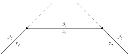
Figure 1.
Schematic picture of the evolution in the mixed “radiation + Cauchy” representation. Traditionally, the “Scri" is drawn as a “light cone”, even if it carries no metric structure.
The initial data on each , therefore, consist of the canonical data on the hyperboloid and the radiation data on the part of the Scri that is situated in the past with respect to , namely . A priori, the evolution of the hyperboloid data is defined only forward in time, whereas the evolution of the radiation data on the half of the Scri is defined only backward in time and consists simply of forgetting the data on this part of the Scri that is skipped when time goes backward. But the system composed of the above two subsystems, interacting via the appropriate corner condition (see [17]) at the intersection
is a genuine Hamiltonian system. Its Hamiltonian functional is equal to the sum of the two energies: the total amount of the “not-yet-radiated” energy contained in (see Formula (51)) and the “already-radiated-energy” given by
(cf. Formula (40)). We have, therefore:
The system is autonomous and the total energy is conserved. But as time increases, the value of the “already-radiated-energy” also increases. In fact, we integrate the positive function over increasing portions of the Scri. In the limit , we obtain the value of the total energy . This means that the “not-yet-radiated-energy” decreases. In the limit , we obtain , i.e., the total energy becomes radiated.
Of course, the hyperboloidal shape of is irrelevant. What really counts is its boundary equal to its intersection with the Scri. It is proved in the next section that the total amount of energy contained in two such hypersurfaces with a common boundary is the same. Hence, lives, in fact, on the 2D section of the Scri. You can simply forget about the 3D hypersurface “filling" it.
9. Quasi-Local Character of the Trautman–Bondi Energy
A similar construction can be performed for generic 2D sections S of the Scri. Denote by the part of the Scri that is situated “before” S. Choose an arbitrary spacelike 3D surface (if any exist) such that null hyperplanes belonging to together with the entire past causal shadow of B, cover the part of spacetime preceeding . If there exists such a , its relation with S will be denoted by . We define as the total field energy contained in , whereas is defined as the total energy radiated “before” s, i.e., contained in . Consider now the evolution consisting of the time shifting of both S and . During this (reversible!) evolution, energy is transferred from subsystem to subsystem . The monotonously decreasing (as time increases) energy , which can be assigned to every 2D section of the Scri, can be called the Trautman–Bondi energy of the scalar field in analogy to the original Trautman–Bondi energy, which describes the energy carried by the gravitational field.
To prove that the theory developed in the previous section really works if we replace with an arbitrary section S of the Scri, we observe that , which we have used above, can also be defined in a different way. Take the 2D sphere:
and a collection of all light rays starting outwards from the points of . Now, is equal to the collection of all null hyperplanes that are tangent to .
Different 2D sections of the Scri can be obtained if we replace the surface (60) with an arbitrary convex 2D surface , not necessarily a round sphere. If again denotes the collection of all light rays starting outwards from the points of , then the collection of all null hyperplanes that are tangent to defines a new 2D section S of the Scri. It can replace our previous section (57) as a “corner surface”, separating the spacelike and the lightlike portions of the new Cauchy surface .
For this purpose take an arbitrary spacelike 3D hypersurface that intersects at S, i.e., satisfying . This simply means that is asymptotically tangent to the “cone” . The group of time translations in the direction of a (previously chosen) time axis (see Formula (24)) becomes a group of canonical transformations, where the phase space is composed of two interacting subsystems: (1) the radiation data on (the part of that lies “in the past of S”), and (2) the canonical data and on the surface . The total Hamiltonian is again equal
where the first term is the amount of energy radiated in the past of S
and the Trautman–Bondi energy equals the integral over of the canonical energy:
where
(observe that H is not a scalar but the scalar density and, therefore, no measure component of the type “” is necessary when integrating it over ). But, geometrically, H is equal to the appropriate component of the canonical energy-momentum tensor density , i.e.,
By the Noether theorem (time translations are symmetries of the theory), the canonical energy-momentum tensor is conserved:
Hence, by the Stokes theorem, the value of the integral (64) does not change if we replace with any other surface that is cobordant to , i.e., satisfying
We conclude that is, in fact, assigned not to a particular 3D hypersurface but to a 2D section S of the Scri. This means that the Trautman–Bondi energy is a quasi-local quantity (this terminology was proposed by R. Penrose much later (see [18])).
Similarly to the case of (57), appropriate corner conditions being fulfilled on S by the Cauchy data— on one side and on the other—imply that the system composed of two subsystems becomes a genuine, autonomous Hamiltonian system. Its total energy remains, therefore, constant during the evolution. But (the “amount of already-radiated-energy”) increases with time, being equal to the integral (61) of a positive quantity over an increasing region . Consequently, the Trantman–Bondi energy, equal to the “amount of not-yet-radiated-energy” (i.e., energy remaining on , where ), decreases as , namely .
10. Role of Boundary Conditions in Hamiltonian Field Theory: Interaction through the Boundary
Both the “formally Hamiltonian” systems of Equations (44)–(45) on the half-Scri and Equations (52)–(53) on the hyperboloid do not separately possess a well-posed initial value problem and, therefore, are not Hamiltonian systems in any rigorous sense. The convenient mathematical criterion here is the self-adjointness of the evolution operator. For example, the evolution (44)–(45) on the Scri is governed by the “momentum” operator , a generator of translations, well known in Quantum Mechanics. This operator is essentially self-adjoint on the whole but has no self-adjoint extension when considered on the half-line (the case of ). Also, canonical energy on the hyperboloid, given by Formula (51), has no self-adjoint extension.
The fact that interaction through the boundary of these two systems restores the self-adjointness if appropriate “corner conditions” are imposed is not a trivial result. But, it is not exceptional. A nice example of this phenomenon is provided by the wave Equation (5) when treated independently on the two complementary half-spaces: the lower one and the upper one . The Laplace operator is not essentially self-adjoint when restricted to a half-space. But, it possesses many inequivalent self-adjoint extensions, each of them defined by a specific boundary condition. Choosing one of them is necessary if we want to treat field evolution within a half-space as an autonomous Hamiltonian system. A priori, such a choice can be made independently for the upper and lower half-spaces.
The conventional field evolution in the whole space can be restored as a Hamiltonian system composed of the above two subsystems, interacting through the common boundary if the following boundary conditions are imposed: the coincidence of the value of the field and the transversal momentum , cf. [13].
We emphasize that these considerations are not empty mathematical toys, but concern the very physical essence of field theory. A purely formal analysis, which can be found in many physical publications, is not sufficient to describe the evolution of the field.
11. Interaction with Sources
The purely linear theory without sources, given by Equation (5), is trivial from the point of view of the “S-matrix", as both the and carry essentially the same information. The non-trivial relation between incoming and outgoing radiation is obtained when there are non-trivial sources on the right-hand side of (5). The sources may appear “deus ex machina”, as external parameters of evolution, or they may be carried by other physical fields (let us denote them by ), interacting non-linearly with our field and constituting, together with , an autonomous, complex physical system . Suppose that the sources vanish outside of a certain world tube
This means that outside the tube, our previous analysis is valid. Hence, Formula (15) defines two different values on every null 3D hyperplane: one for , which we assign to a point , and another for , which we assign to the corresponding point . The difference between these two values describes the amount of energy that has been transferred from the subsystem to the subsystem (or vice versa if the value is negative) during the evolution of the complex system .
It should be noted that the assumption (67) regarding the spatial localization of sources is probably too restrictive. Indeed, this rules out a situation in which the sources are carried by a “small material body” moving freely (i.e., along a straight, timelike trajectory) before and after a finite time interval while the interaction was active. But also in this case, each null 3D hyperplane enters for and for into the region where the sources disappear and our construction works correctly.
12. Maxwell Field and the Linearized Gravity
Every linear, hyperbolic field theory can, finally, be reduced to a system of a few, decoupled, wave equations. In electrodynamics, such a reduction (compatible with the symplectic reduction of the phase space of Cauchy data with respect to constraints: ), is not unique. A version that is especially useful for our purposes is based on a choice of spherical coordinates It is easy to prove that both fields, and , where and are radial components of the electric and magnetic fields, respectively, satisfy the wave Equation (5) as a consequence of the Maxwell equations (we use the below Cartesian coordinates :
which is the same for . The role of conjugate momenta is played by the radial components of the “curl”:
which carry information about . Moreover, the complete information about the fields and can be reconstructed from the canonical data in a quasi-local way, i.e., solving the 2D Poisson equation on each sphere separately.
A similar reduction can be applied in the case of the linear version of Einstein’s gravity theory. Here, the dynamical variables can be described by 10 independent components of the linearized Weyl tensor:
(see [19]), which can be encoded by two independent, symmetric TT tensors (traceless, transversal):
It turns out that the entire dynamics of this field can be again reduced to the wave Equation (5) for two independent degrees of freedom: and (see [19,20]). The corresponding canonical momenta are again given as the radial part of the “curl”, namely:
and, moreover, the complete information about both fields, and , can be reconstructed from the canonical data in a quasi-local way, i.e., by solving the 2D Poisson equation on each sphere separately (see [21,22,23]). Consequently, our theory of radiation, when applied to canonical variables, , can also describe the radiation carried by the Maxwell field and gravitational field in the linear approximation.
13. Gravitational Radiation Theory
In our description of the radiation phenomena, we have explicitly used the flat (affine) structure of the Minkowski spacetime. We cannot apply this technique a priori to describe the gravitational radiation that occurs in a curved spacetime M. Fortunately, the basic scheme of radiation theory outlined above remains valid if we assume that this curved spacetime is asymptotically flat. Physically, asymptotic flatness means that the gravitational system that we analyze is isolated. Technically, we assume that there is a spatially bounded world tube T (the “strong-field-region”, cf. (67)) such that outside of it (i.e., in the “weak-field-region” ), the metric can be written as , where is the flat Minkowski metric, whereas its perturbation h behaves like and the connection coefficients behave like .
In an asymptotically flat spacetime M, asymptotic structures at infinity can be described in a perturbative way. For this purpose, we use the linearized version of the General Relativity Theory, which reduces to two wave equations describing the evolution of the two independent degrees of freedom. As described in Section 12, these degrees of freedom can be chosen in a gauge-invariant way as the two independent components of the linearized Weyl tensor (see [21,22]). Linearized Einstein equations reduce them to two independent wave equations. They describe the evolution of the gravitational field only approximately. But this approximation improves the further we move away from the strong field region T. Because radiation takes place at infinity, the quantities that live on the Scri are rigorously described in terms of the linear theory! Hence, is rigorously described by Formula (61), and the Trautman–Bondi energy is a quantity associated with every section S of the Scri.
What is not rigorous when we limit ourselves to the linear theory, is the description of energy in finite regions. We cannot, therefore, expect any formula similar to (62), where the energy density H would be spread over a spacelike surface . There is no such energy density because gravitational energy is not additive. Indeed, if such a density existed, the amount of energy contained in a 3D volume V would be equal to
If V is divided into a sum of two disjoint subsets, , then (72) implies that . But such an additivity of gravitational energy contradicts the very notion of gravitation. The energy weights (in fact, it is equal to its mass!) and, consequently, their interaction energy cannot vanish:
This conclusion is nothing but Newton’s law of universal gravitation!
Fortunately, gravitational energy is quasi-local. This means that the amount of Trautman–Bondi energy assigned to each 2D section S of the Scri is given by a surface integral already in the complete non-linear theory, similar to the case of the A.D.M energy at space infinity (cf. [24]). Hence, the purely special-relativistic considerations based on the Noether theorem and the “conservation” of energy-momentum tensor-density (which was the case in (64) and (65)) are not necessary here. As a consequence, the entire Hamiltonian theory of gravitational radiation, defined by the asymptotically linearized theory, works perfectly well.
14. Geometric Description of the Scri in an Asymptotically Flat Spacetime
What remains is the relation of the asymptotic objects defined with the use of the (totally artificial!) flat Minkowski metric and the real geometric objects living in the physical, non-flat spacetime M. The flat null “hyper-planes ” do not exist in curved spacetime and, therefore, we cannot use them to represent Scri points.
To define such a representation in terms of the intrinsic, geometric objects living in M, we begin with the original idea of the “asymptotic value of the field on the light ray”:
where
is a parametrization of a light ray L and is a “laboratory time”, i.e., the time coordinate in any asymptotically flat coordinate chart , as described in Section 13 (cf. Formula (11)). The value , defined by (74), does not depend on the choice of the “initial time” because
As was obvious in the case of a flat M, the same value is obtained for the entire “equivalence class” of light rays. The collection s of all those “equivalent” right rays constitutes a null 3D surface and represents a point of the Scri. In the flat case, such a surface was flat. In a generic case, at most, “asymptotic flatness” can be expected. Below, we briefly outline the idea of the construction of such surfaces.
Given a light ray L and a point , situated “far away” from the strong field region T, choose a 2D spacelike tangent subspace in . The collection of all geodesic lines that begin at x whose tangent vector belongs to P generates a 2D surface . Finally, the parallel transport of the null vector tangent to L at x enables us to choose at each point of a null geodesic. The collection of all of them generates the 3D null surface . If the physical metric is “almost flat” (i.e., the perturbation h is “almost null”), then the resulting surface is “almost flat”. The surface that represents a point of the Scri is the (appropriately defined) limit of surfaces when , i.e., when the entire construction is performed in an “almost flat” surrounding. We limit ourselves here to present only the idea of this theory, and the technical details will be presented in another paper.
Funding
This research received no external funding.
Data Availability Statement
Data are contained within the article.
Conflicts of Interest
The author declares no conflict of interest.
Appendix A. Wave Equation and the Huygens Formula
Given a function on a 3D Euclidean space, we define
for every real number . The new function is regular on (its regularity class is equal to the class of f). Observe that this is even with respect to the time variable:
Hence, is equal to the mean value of f taken on the sphere centered at , whose radius r is equal to .
Observe that rigid translations of the function f commute with calculating its mean value over a sphere. The infinitesimal version of this observation can be formulated as follows: for every 3D vector , the following identity holds:
Hence, the same applies to the Laplacian operator:
The second equality holds because when expressed in spherical coordinates centered at , the angular part of vanishes when integrated over the sphere. On the other hand, we have an obvious identity
which, when applied twice, proves immediately that the function
fulfills the following partial differential equation:
This implies that satisfies the wave Equation (5). We conclude that from every 3D function f, we can manufacture a solution of the wave equation:
But a derivative of a solution is also a solution, i.e.,
is also a solution. It is easy to prove that every solution is a sum of two such solutions:
which is a decomposition of into an even (first) and odd (second) part with respect to the time variable , whereas and are Cauchy data taken at .
References
- Einstein, A. Näherungsweise Integration der Feldgleichungen der Gravitation; Sitzungsberichte; Preussische Akademie der Wissenschaften: Berlin, Germany, 1916; Part 1; pp. 688–696. [Google Scholar]
- Einstein, A. Gravitationswellen; Sitzungsberichte; Preussische Akademie der Wissenschaften: Berlin, Germany, 1918; Part 1; pp. 154–167. [Google Scholar]
- Einstein, A.; Rosen, N. On gravitational waves. J. Frankl. Inst. 1937, 223, 43–54. [Google Scholar] [CrossRef]
- Kennefick, D. Traveling at the Speed of Thought: Einstein and the Quest for Gravitational Waves; Princeton University Press: Princeton, NJ, USA, 2007; Chapter 5. [Google Scholar]
- Hill, C.D.; Nurowski, P. How the green light was given for gravitational wave research. arXiv 2017, arXiv:1608.08673v1. [Google Scholar]
- Trautman, A. Boundary conditions at infinity for physical theories. Bull. Acad. Polon. Sci. 1958, 6, 403–406. [Google Scholar]
- Trautman, A. Radiation and boundary conditions in the theory of gravitation. Bull. Acad. Polon. Sci. 1958, 6, 407–412. [Google Scholar]
- Trautman, A. Lectures on General Relativity; Mimeographed Notes; King’s College London: London, UK, 1958. [Google Scholar]
- Arnowitt, R.; Deser, S.; Misner, C. Dynamical Structure and Definition of Energy in General Relativity. Phys. Rev. 1959, 116, 1322–1330. [Google Scholar] [CrossRef]
- Arnowitt, R.; Deser, S.; Misner, C. The Dynamics of General Relativity. In Gravitation: An Introduction to Current Research; Witten, L., Ed.; Wiley: New York, NY, USA, 1962; p. 227. [Google Scholar]
- Chruściel, P.; Jezierski, J.; Kijowski, J. Hamiltonian Field Theory in the Radiating Regime; Springer Lecture Notes in Physics, Monographs; Springer: Berlin/Heidelberg, Germany, 2001; Volume 70, 174p. [Google Scholar]
- Szabados, L.B. Quasi-Local Energy-Momentum and Angular Momentum in GR: A Review Article. Living Rev. Relativ. 2004, 7, 4. [Google Scholar] [CrossRef] [PubMed]
- Kijowski, J.; Tulczyjew, W.M. A Symplectic Framework for Field Theories; Lecture Notes in Physics No. 107; Springer: Berlin/Heidelberg, Germany, 1979. [Google Scholar]
- Białynicki-Birula, I.; Białynicka-Birula, Z. Quantum Electrodynamics, 1st ed.; Pergamon Press: Oxford, UK, 1975. [Google Scholar]
- Bogoliubov, N.N.; Shirkov, D.V. Introduction to the Theory of Quantized Fields; John Wiley & Sons: Hoboken, NJ, USA, 1980. [Google Scholar]
- Souriau, J.-M. Structure des Systemes Dynamiques; Dunod: Paris, France, 1970. [Google Scholar]
- Kijowski, J.; Chmielowiec, W. Hamiltonian description of radiation phenomena: Trautman-Bondi energy and corner conditions. Rep. Math. Phys. 2009, 64, 223–240. [Google Scholar]
- Penrose, R. Quasilocal mass and angular momentum in general relativity. Proc. R. Soc. Lond. 1982, A381, 53–63. [Google Scholar]
- Kijowski, J.; Jezierski, J.; Wiatr, M. Localizing energy in Fierz-Lanczos theory. Phys. Rev. 2020, D102, 024015. [Google Scholar]
- Jezierski, J.; Kijowski, J.; Waluk, P. Gauge-invariant quadratic approximation of quasi-local mass and its relation with Hamiltonian for gravitational field. Class. Quantum Gravity 2021, 38, 095006. [Google Scholar] [CrossRef]
- Jezierski, J. The Relation between Metric and Spin-2 Formulations of Linearized Einstein Theory. Gen. Relativ. Gravit. 1995, 27, 821–843. [Google Scholar] [CrossRef]
- Jezierski, J. “Peeling property” for linearized gravity in null coordinates. Class. Quantum Gravity 2002, 19, 2463–2490. [Google Scholar] [CrossRef]
- Jezierski, J. CYK tensors, Maxwell field and conserved quantities for spin-2 field. Class. Quantum Gravity 2002, 19, 4405–4429. [Google Scholar] [CrossRef][Green Version]
- Kijowski, J. A simple derivation of canonical structure and quasi-local Hamiltonians in general gelativity. Gen. Relat. Grav. 1997, 29, 307. [Google Scholar] [CrossRef]

Disclaimer/Publisher’s Note: The statements, opinions and data contained in all publications are solely those of the individual author(s) and contributor(s) and not of MDPI and/or the editor(s). MDPI and/or the editor(s) disclaim responsibility for any injury to people or property resulting from any ideas, methods, instructions or products referred to in the content. |
© 2023 by the author. Licensee MDPI, Basel, Switzerland. This article is an open access article distributed under the terms and conditions of the Creative Commons Attribution (CC BY) license (https://creativecommons.org/licenses/by/4.0/).