DPQP: A Detection Pipeline for Quasar Pair Candidates Based on QSO Photometric Images and Spectra

Abstract

Quasars have an important role in the studies of galaxy evolution and star formation. The rare close projection of two quasars in the sky allows us to study the environment and matter exchange around the foreground quasar ($QS{O}_{fg}$) and the background quasar ($QS{O}_{bg}$). This paper proposes a pipeline DPQP for quasar pair (QP) candidates’ detection based on photometric images and the corresponding spectra. The pipeline consists of three main parts: a target source detector, a regressor, and a discriminator. In the first part, the target source detection network–YOLOv4 (TSD-YOLOv4) and the target source classification network (TSCNet) are used in sequence to detect quasars in SDSS photometric images. In the second part, a depth feature extraction network of quasar images (DE-QNet) is constructed to estimate the redshifts of quasars from photometric images. In the third part, a quasar pair score (Q-Score) metric is proposed based on the spectral analysis. The larger the Q-Score, the greater the possibility of two pairs being a quasar pair. The experimental results show that between redshift 1.0 and 4.0, the MAE of DE-QNet is 0.316, which is 16.1% lower than the existing method. Samples with |$\Delta$z| < 0.15 account for 77.1% of the test dataset. A new table with 1025 QP candidates is provided by traversing 50,000 SDSS photometric images.

1. Introduction

The quasar is an extremely bright active galactic nucleus (AGN), known as one of the most powerful and energetic objects in the universe [1]. Its activity represents a brief energetic phase in galaxy evolution, which plays a vital role in galaxy evolution and star formation [2]. In particular, two quasars that are within a certain distance and interact with each other are called a quasar pair in astronomy [3]. For a QP, a background quasar can be used to study a foreground quasar’s halo gas in absorption, providing a wealth of information about feedback, quenching, and the physics of massive galaxy formation [4]. These unique sightlines allow us to study the quasar circumgalactic medium (CGM) in absorption and emission simultaneously, because the background quasar pinpoints large concentrations of gas [5]. There has been much speculation that some feedback mechanism links a quasar at a particular stage to the evolution of its host galaxy [6,7,8]. A QP is of great assistance in the study of quasars and their physical environments. Therefore, in the field of astronomy, the search for QPs is of extraordinary importance.

A QP is a rare close projection of two quasars in the sky [9]. Artificial authentication is the basic way to confirm a QP, provided that both quasars have the observed spectra. However, fiber collisions1 largely prevent the simultaneous observation of objects with separations <55” in the SDSS spectrometer, which poses a great challenge to artificial authentication. With the increase in the number of astronomical telescopes and the development of technology, astronomical observations have entered the big data era, such as SDSS [10], Pan-STARRS [11], DES [12], and JWST [13]. At the same time, machine learning methods have been increasingly applied in the field of astronomy, such as the target source detection task (e.g., Refs. [14,15,16,17]), and the quasar redshift estimation task (e.g., Refs. [18,19,20]) in recent years. The objective of the work in this paper is to construct a pipeline for QP candidates’ detection based on photometric images and spectra.

The pipeline consists of three parts: a target source detector, a regressor, and a discriminator. Part one (target source detector): the quasar detection algorithm selects a two-stage network, first utilizing a detection algorithm (TSD-YOLOv4) to identify target sources in SDSS images, and then (TSCNet) classifying the target sources to obtain quasars. Part two (regressor): it is increasingly common to use photometric images to estimate redshifts in regression tasks. However, quasars appear similar to stars in images and have a less diverse color compared to stars. Former methods cannot extract accurate morphological information about quasars, resulting in poor redshift regression. To address these problems, we design a quasar redshift estimation network (DE-QNet) to estimate the detected quasar redshift. Part three (discriminator): the spectra of quasars present in the images are obtained from the CasJobs Server and used as background quasars for neighborhood matching with the detected quasars. For the screened neighboring QP, we propose a metric (Q-Score) based on spectral analysis. The Q-Score represents the interaction intensity between two quasars. The target source detector (TSD-YOLOV4 and TSCNet) achieves a high accuracy source localization and classification task; the regressor (DE-QNet) achieves a low MAE quasar redshift estimation task; and the discriminator screens QP candidates based on spectral analysis. According to this idea, we propose a QP candidate detection pipeline (DPQP). The overall structure is shown in Figure 1.

The organization of this paper is as follows: Section 2 describes the data and data processing method in this paper. Section 3 introduces and discusses the target source detector and regressor (DE-QNet). Section 4 introduces the metric Q-Score and describes the spectral analysis process. Section 5 analyzes and discusses the experimental results of the DE-QNet and DPQP. Section 6 summarizes the experimental results and findings, and the QP candidates’ table is provided in Appendix A.

2. Data

This paper uses the 17th data release (DR17) of the Sloan Digital Sky Survey (SDSS). The SDSS uses charged coupled device (CCD) filters to observe the sky and collect photometric images in five bands: u, g, r, i, and z. The corresponding central wavelengths of each band are 3551 Å, 4686 Å, 6166 Å, 7480 Å, and 8932 Å, respectively [21]. Most work tasks use data from the u, g, r, and i bands, while the z band, which has high noise, is often discarded. Because different bands of data contain different information, in order to fully utilize all the information in the image, we use all five bands of data as input for the network.

This paper combines the SpecObjAll and PhotoObjAll catalogs and uses SQL statements to query the data in CasJobs Server. As shown in Figure 2a, we cross-reference the data on CasJobs Server and find that the quasars’ number in Z > 3.0 is about 56,000, and the one in Z < 3.0 is about 810,000. However, the dataset sample distribution is severely uneven and can lead to the neural network focusing on the samples with a larger number. Therefore, to make the data distribution more reasonable, this paper samples the data evenly and obtains a total of 76,000 spectra; a total of 75,915 quasar samples are eventually screened by further removing samples from a number of contaminating sources (refer to Figure 2b). This dataset is randomly divided into three parts: the training set, the validation set, and the test set, which account for 70%, 20%, and 10% of the entire dataset, respectively.

3. Method

The DPQP consists of 3 parts in Figure 1: target source detector, regressor, and discriminator. The target source detector is a reusable work task described in detail in paper [17]. Section 3.1 provides a brief introduction to TSD-YOLOv4 and TSCNet. Section 3.2 describes DE-QNet’s structure and details.

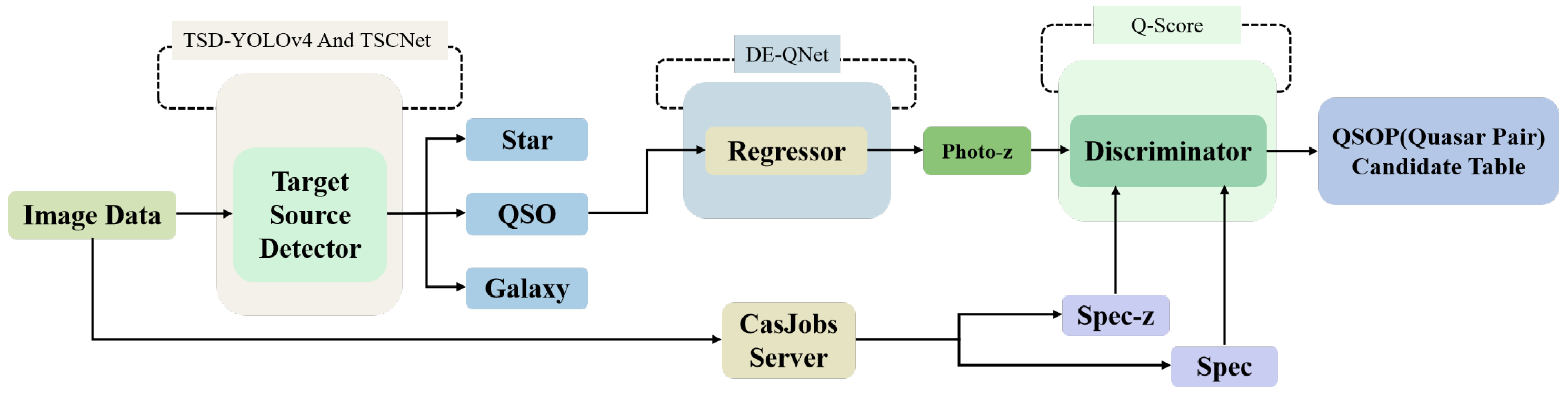
3.1. Target Source Detector

In this paper, TSD-YOLOv4 is selected as the target detection network. It has the best detection results compared to typical networks such as SSD, CenterNet, Faster-RCNN, YOLOX, and YOLOv4. TSD-YOLOv4 achieves an accuracy of 0.988 and a recall of 0.997 on 11,808 target source detection samples. TSCNet is selected as the source classification network. It has a precision of 0.908 for quasars and a recall of 0.903 in a classified sample of 232,816: 106,547 galaxies, 64,236 quasars, and 62,033 stars. This method yields 2–3% more sources than the SDSS PhotoObjAll catalog ones that are not included in the SDSS, which may include quasars.

3.2. Regressor

Section 3.2.1 describes the various modules of DE-QNet and their functions. Section 3.2.2 describes the training strategy of DE-QNet.

3.2.1. Redshift Estimation Network: DE-QNet

In photometric images, quasars are always presented as homochromatic point sources, which means that image features are not well extracted. Refs. [20,22] proposed a method that had few network layers and poor accuracy. In order to better extract the image features, a deep neural regression network DE-QNet was designed, which balances network depth and accuracy. The DE-QNet structure is shown in Figure 3, and the network parameters are shown in

Table 1. DE-QNet parameter table.

Layer	Output Size	Input Channels	Output Channels	Kernel Size	Stride	Padding	Activation
P1	64 × 64	5	32	3	1	1	Hardswish
P2	32 × 32	32	64	3	2	1	Hardswish
P3	32 × 32	64	64	3	1	1	Hardswish
P4	16 × 16	64	64	2	-	-	-
P5	16 × 16	64	128	3	1	1	Hardswish
P6	16 × 16	128	256	-	-	-	-
P7	8 × 8	256	256	-	-	-	-
P8	8 × 8	256	64	1	1	1	Hardswish
Fully connected	-	4096	1024	-	-	-	Hardswish
Fully connected	-	1024	32	-	-	-	Hardswish
Fully connected	-	32	1	-	-	-	Hardswish

.

The input of DE-QNet is the five-band photometric images, and the output is the quasar redshift estimation. DE-QNet consists of many CBH modules, 3 CGH modules, a downsampling layer, an SCP module, a DM (Double Max-pooling) module, and 3 fully connected layers.

The CBH module is made up of convolution, batch normalization (BN), and a hardswish activation function. The CGH module is made up of convolution, group normalization (GN), and a hardswish activation function. The SCP module consists of four CBH modules and a CGH module. Feature fusion is achieved through a first layer of 1 × 1 convolution, a second layer of 3 × 3 convolution, and a fourth layer of 3 × 3 convolution, and the fused features have a depth of three times the number of channels. Finally, a 1 × 1 convolution layer is added to squeeze the channel dimension from three times to one time. The DM module uses Maxpool2d parallel to the CBH module for downsampling of the images.

In the second layer of the network (P2), no pooling layer is used after the convolution layer step as in classical networks. The pooling layer is mainly used to remove redundant information and reduce overfitting. Its effect on the image is to reduce the size of the original image by half. However, it is difficult to extract image features from quasar images. In order to further extract image features, this paper replaces the pooling layer with a convolution layer (stride = 2, padding = 1) to perform convolution on the image again to extract image features. The output image size is the same as the output image size using the pooling layer, reducing the number of parameters. In the fourth layer of the network (P4), a pooling layer (Maxpool2d) is added to reduce overfitting. When the network reaches a certain depth, the accuracy gain becomes smaller and smaller if the computational blocks continue to be stacked. What is worse is that when the network reaches a certain critical depth, its convergence begins to deteriorate, resulting in lower overall accuracy compared to shallow networks. This paper uses a gradient path design strategy to design SCP modules (P6) for layer aggregation architectures with efficient gradient propagation paths. The SCP module not only achieves feature fusion, but also reduces network depth, thereby further extracting the characteristics of quasar point sources. Afterward, downsampling is performed through the DM module, which reduces the parameter count and also extracts features.

3.2.2. Network Training Strategy

The programming language is Python. The hardware parameters for the experiments are [email protected] CPU and NVIDIA GeForce RTX 1650 Ti GPU. Before training the network, some hyperparameters need to be set in advance, such as batch size, learning rate, epochs, etc.

Table 2. Hyperparameter configuration of DE-QNet.

Configuration	DE-QNet
Optimizer	Adam
Batch size	8
Totale poch	300
Learn rate	1 × 10${}^{-4}$
Resize shape	64

summarizes the parameter configuration for the DE-QNet module.

The DE-QNet module uses mini-batch training during the training process. Most current training network strategies add a BN layer before the activation function to accelerate the convergence of the network. However, excessive BN layers can result in the accumulation of error offsets, which is described in detail in [23]. The paper proposes an ABA configuration: substituting the BN layer of the middle convolution with GN, layer normalization (LN), or instance normalization (IN) layers when three consecutive convolutions appear, which can effectively reduce error accumulation. This paper proposes the CGH module. GN layers require mini-batch training; therefore, this paper adopts a batch size of 8.

4. Discriminator

In this section, we describe the QP determination process. The photometric image redshift, spectral redshift, and spectra are used as the input to the discriminator. The Q-Score is obtained from the spectral analysis, which represents the intensity of the interaction between the two quasars. The larger the Q-Score is, the more likely it is to determine a QP. Section 4.1 describes the method for defining the Q-Score. Section 4.2 describes the spectral analysis process.

4.1. Q-Score Indicator

If two quasars constitute a QP, then there will be a series of clearly visible absorption lines in the background quasar spectrum. These absorption lines correspond to the emission lines in the spectra of foreground quasars. Assuming that the two quasars have similar z, this relationship is: when photons from the background quasar pass through the foreground quasar halo, a part of the photon energy is absorbed by the foreground quasar, resulting in a corresponding absorption line in the background quasar spectrum. This relationship is represented on the spectrum as: the background quasar absorption line corresponds to the foreground quasar emission line. The evaluation metric Q-Score represents the degree of intensity of this relationship on the spectrum. Ref. [24] upgraded the SDSS spectrometer by extending the observation wavelength range covered by the input spectra from 3800–9200 Å to 3600–10,400 Å. The primary rest-frame ultraviolet quasar emission lines that are redshifted into the optical for Z ≥ 2 quasars are: Ly$\alpha$ $\lambda$1216, N V $\lambda$1240, C IV $\lambda$1549, C III] $\lambda$1908, and Mg II $\lambda$2798.

In order to ensure the appearance of Ly$\alpha$ and Mg II emission lines in the spectrum, some restrictions are imposed on the redshift of the background quasar. For the blue side, starting at wavelength ${\lambda }_{obs}$ = 3600 Å, according to ${\lambda }_{obs}$ = (1 + $Z_{bg}$) × 1215.86, $Z_{bg}$ = 1.97 is the minimum redshift value at which the Ly$\alpha$ emission line appears in the spectrum. For the red side, the ending at wavelength ${\lambda }_{obs}$ = 10,400 Å, according to ${\lambda }_{obs}$ = (1 + $Z_{bg}$) × 2800.14, $Z_{bg}$ = 2.71 is the maximum redshift value at which the Mg II emission line disappears from the spectrum. In order to accurately detect Ly$\alpha$ absorption, the quasar of the Z ≥ 2.1 is selected as the background quasar to detect the foreground quasar. At Z > 2.71, the Mg II emission line disappears from the spectrum; to increase accuracy, the Ly$\beta$ emission line needs to be considered for observation. The NV emission line is abandoned because the mixing of the NV emission line with the Ly$\alpha$ emission line is not good, and it can only be detected when the NV line is very sharp.

The final selection includes seven emission lines, which consist of five strong emission lines: Ly$\beta$, Ly$\alpha$, C IV, C III, and Mg II, as well as two weak emission lines: O I and Si IV. The emission line information is shown in Table 3, and the Q-Score metric formula is shown in Equation (1). In Equation (1), $N_x$ represents whether the emission line is identified (with a value of 0 or 1), and its weight is based on the relative flux values in Table 2 of [25]. In Table 2 of [25], the relative flux of Ly$\alpha$ is 100% because all other emission lines are compared to the Lya line as a reference. However, due to the excessively large relative flux of Ly$\alpha$, this would result in the minimal impact of other emission lines on the Q-Score. Considering the importance of Ly$\alpha$ when discriminating the significance of QP, we decide to assign a weight of 50% to maintain the influence of Ly$\alpha$ on the Q-Score while keeping the relative flux of other emission lines unchanged. As a result, the relative influence of other emission lines increases, while the influence of Ly$\alpha$ decreases relatively but still holds a significant proportion.

Table 3. Quasar emission line selection and corresponding wavelengths.

Emission Lines	$\mathsf{\lambda }$
Ly$\beta$	1031.48
Ly$\alpha$	1215.86
O I	1305.31
Si IV	1398.16
C IV	1545.57
C III	1903.61
Mg II	2800.14

Table 3. Quasar emission line selection and corresponding wavelengths.

Emission Lines	$\mathsf{\lambda }$
Ly$\beta$	1031.48
Ly$\alpha$	1215.86
O I	1305.31
Si IV	1398.16
C IV	1545.57
C III	1903.61
Mg II	2800.14

$$\begin{array}{c}f\left(x\right)=\left\{\begin{array}{cc}{N}_{Ly\beta }\times 9.615+N_{Ly\alpha }\times 50+N_{OI}\times 1.992+N_{SiIV}\times 8.916+N_{CIV}\times 25.291+N_{CIII}\times 15.943\hfill & 2.67\le z\le 4.00\hfill \\ N_{Ly\alpha }\times 50+N_{OI}\times 1.992+N_{SiIV}\times 8.916+N_{CIV}\times 25.291+N_{CIII}\times 15.943+N_{MgII}\times 14.725\hfill & 2.10\le z\le 2.67\hfill \end{array}\right.\hfill \end{array}$$

(1)

4.2. Spectral Analysis Process

This section describes the process with regard to spectral analysis. The method of removing the continuum and filtering is used to highlight the spectrum’s absorption/emission line features. Section 4.2.1 describes the removal of the continuum. Section 4.2.2 describes a new approach to filtering.

4.2.1. Spectral Analysis Process

The spectrum of a quasar is different from any other astronomical object, usually with extremely strong emission and absorption lines. In order to highlight the absorption and emission line features of the quasar, the method in [26] is selected to remove the continuum. QP J0036 + 0839, as an example, shows processing of its $QS{O}_{bg}$ J003643.45 + 083944.40 spectrum. The spectrum after processing is shown in Figure 4, where the absorption lines’ positions can be highlighted.

4.2.2. Filtering

For most of the quasar spectra, their signal-to-noise (SNR) are low. Thus, some spectral features are destroyed because of cosmic rays, noise, and other factors. In order to better find the location of the absorption lines, a filtering operation on the spectrum is necessary. In this paper, we propose a multistage hybrid filtering method, the structure of which is shown in Figure 5. The multistage hybrid filter consists of two mean filters and a median filter. The mean filter is linear filtering that uses the average value of the target and its neighboring values to smooth out the data and reduce noise. Its disadvantage is that it cannot preserve data details well. Although it can effectively suppress noise, it may filter out prominent absorption line features. The median filter is nonlinear filtering, which can preserve the absorption line features well when smoothing the spectral lines but cannot suppress the noise much. Combining them can complement each other and achieve better filtering results.

As shown in Figure 6, the red line represents the spectrum after undergoing filtration with a multistage hybrid filter; the blue line corresponds to the spectrum that has solely passed through the process of removing the continuum. As shown in Figure 6a, the red line preserves the relative strength of the absorption lines well. As shown in Figure 6b,c, the red line fits the positions of the absorption lines well and smooths the spectrum, making it easier to identify the absorption lines.

4.2.3. Searching for Absorption Lines

The location of the absorption line is searched easily through the filtered spectrum. The SciPy library from the Python toolkit is used to search for the absorption line. Figure 7 shows a close-up of the original spectrum (blue line) and the processed spectrum (red line) of $QS{O}_{bg}$ J003643.45 + 083944.40; the symbol ‘X’ represents the location of the possible absorption line. It can be seen that most of the absorption lines have been identified.

By the method proposed in Section 4.2, QP J0036 + 0839 is used as an example. Figure 8 shows the original spectrum (blue line) and the processed spectrum (red line) of $QS{O}_{bg}$ J003643.45 + 083944.40 at a redshift of Z = 2.690. The “X” on the red line indicates the location of the absorption line. To assess the accuracy of absorption line identification, we utilize $QS{O}_{fg}$ J003653.85 + 083936.20 (green line) at a redshift of Z = 2.565 for observation. It can be seen that an absorption line marked with an ‘X’ symbol is found near the emission line (purple line). Among them, C III is not searched, and it is possible that the C III emission line from $QS{O}_{fg}$ does not cause absorption on $QS{O}_{bg}$.

5. Results and Discussion

This section is divided into four subsections. Section 5.1 and Section 5.2 discuss and analyze the DE-QNet experimental results, while Section 5.3 and Section 5.4 discuss and analyze the DPQP experimental results. In Section 5.1, the evaluation metrics of DE-QNet are shown. Section 5.2 analyzes and discusses the performance of DE-QNet. Section 5.3 provides an example to illustrate the DPQP process. Section 5.4 uses the DPQP on discovered QPs and discusses the analysis. The target source detector uses a proven algorithm, which is discussed and analyzed in detail in [17].

5.1. Evaluation Metrics

Evaluation metrics are very important in deep learning because they can evaluate the model performance and the accuracy of prediction results. In this paper, mean squared error (MSE), mean absolute error (MAE), the mean of $\Delta$z (Bias), normalized median absolute deviation (NMAD), and ${\delta }_{0.3}$ are used for evaluating the network performance.

$$\mathrm{MSE}=\frac{1}{N}\sum _{i=1}^N{\left(z_i-{\widehat{\mathrm{z}}}_i\right)}^2$$

(2)

$$\mathrm{MAE}=\frac{1}{N}\sum _{i=1}^N\left|z_i-{\widehat{\mathrm{z}}}_i\right|$$

(3)

MSE is the average squared difference between the predicted values and the actual values. MAE is the average absolute difference between the predicted values and the actual values. N is the number of samples. $z_i$ (Spec-z) is the spectral redshift value of the sample; ${\widehat{z}}_i$ (Photo-z) corresponds to the predicted redshift value.

$$\Delta \mathrm{z}=\frac{z_i-{\widehat{\mathrm{z}}}_i}{1+z_i}$$

(4)

$$Bias=Mean(\Delta \mathrm{z})$$

(5)

$$\sigma (\Delta \mathrm{z})=\sqrt{\frac{1}{\mathrm{n}}\sum _{\mathrm{i}=1}^{\mathrm{N}}{\left(\Delta {\mathrm{z}}_{\mathrm{i}}-\mathrm{Bias}\right)}^2}$$

(6)

|$\Delta$z| is the normalized difference between the true value and the estimated value. Bias is the mean value of |$\Delta$z|, and $\sigma (\Delta \mathrm{z})$ is the standard deviation of |$\Delta$z|.

$$NMAD=1.48\times Median\left(\right|\Delta \mathrm{z}\left|\right)$$

(7)

NMAD is a statistic used to evaluate the level of dispersion of outliers in a dataset, and it is advantageous when dealing with datasets that have outliers or non-normal distributions. Compared to the standard deviation $\sigma (\Delta \mathrm{z})$, NMAD is less sensitive to outliers, providing a more reasonable estimate of the results. The factor 1.48 is a scaling factor that makes NMAD equivalent to the standard deviation of normal distribution data.

$${\delta }_{\mathrm{A}}=\frac{{\mathrm{N}}_{|\Delta \mathrm{Z}|}<\mathrm{A}}{{\mathrm{N}}_{\mathrm{total}}}$$

(8)

${\mathrm{N}}_{|\Delta \mathrm{Z}|}<\mathrm{A}$ represents the number of samples whose |$\Delta$z| is less than A, while ${\mathrm{N}}_{\mathrm{total}}$ is the total number of samples.

5.2. Comparison and Analysis of DE-QNet

This section discusses the experimental results based on the estimation of photometric image redshift and illustrates the advantage of DE-QNet proposed in this paper. The trained model is tested on 7516 untrained and unvalidated quasar images to evaluate the reliability of the model. All data in the paper are SDSS photometric images, and the input images are five bands data from SDSS.

Table 4. The performance of DE-QNet compared with other regression networks. Smaller MSE, MAE, $\sigma (\Delta z)$, NMAD are preferable; smaller absolute value of bias is preferable; larger ${\delta }_{0.3}$ is preferable.

Method	MSE	MAE	Bias	$\mathsf{\sigma }(\mathbf{\Delta }\mathit{z})$	NMAD	${\mathsf{\delta }}_{0.15}$	${\mathsf{\delta }}_{0.3}$
DCMDN	0.387	0.389	−0.052	0.299	0.117	0.682	0.894
NetZ	0.299	0.367	−0.048	0.267	0.124	0.680	0.868
DE-QNet	0.284	0.316	−0.048	0.264	0.081	0.771	0.888

presents the performance comparison of DE-QNet with other regression networks, where the evaluation metrics are presented in Section 5.1. It can be seen that DE-QNet is the best in all metrics and shows a marked improvement compared to DCMDN and NetZ. Compared to DCMDN, DE-QNet reduces the MSE and MAE by 26.6% and 16.4%, respectively. Compared to NetZ, DE-QNet reduces the MSE and MAE by 5.6% and 14.5%, respectively. This indicates that the predicted values are closer to the label values and have smaller absolute errors. To observe the predicted distribution of the redshift of the quasar images, the density maps of the label and predicted redshifts are plotted, as shown in Figure 9.

As shown in Figure 9, as the density increases, the color becomes redder, while as the density decreases, the color becomes bluer. The blue dashed line in Figure 9 shows the sample points whose |$z_i$−${\widehat{z}}_i$| ≥ 0.3, accounting for 88.8% of the total test set. According to Figure 9, it can be seen that there are relatively fewer scattered points in the low redshift (0–0.5) and high redshift (2.2–4), which represents lower prediction errors compared to the mid-redshift (1.9–2.2). Although there are many works on quasar redshift regressions ([19,20,22]), the sample results in the (0.5–0.9) and (1.9–2.2) ranges cannot come close to the desired results. This range may be improved by photometric redshift optimization, but the prediction error in this paper is still the lowest among the image estimation methods.

5.3. DPQP Processing

This section describes the DPQP processing in terms of QP J1204 + 0221. Figure 10 shows J1204 + 0221 in the SDSS image at run = 1458, camcol = 3, field = 376; the background quasar redshift ($Z_{bg}$) is 2.528; the foreground quasar redshift ($Z_{fg}$) is 2.436; and the pair members are separated by an angular distance of $\theta$≃ 13.3 arcseconds on the sky. However, only the former has the corresponding spectral data in the DR17 database of SDSS (Figure 10a blue box), while the latter does not, so confirming that the QP needs to cross multiple databases. In this way, searching for a large number of QPs is complex and labor-intensive, so it would be valuable to detect QP candidates using images. The imaging method used in this paper still tries to select QP candidates based on the principle that the closer the distance, the more effective it is. Specifically, the method is divided into nine steps:

• Step 1: Detecting the target sources in the image, with the detection of quasars as the $QS{O}_{fg}$.
• Step 2: The CasJobs Server obtains quasars with spectra in this image as $QS{O}_{bg}$ (red boxes in Figure 11) and matches these $QS{O}_{bg}$ with $QS{O}_{fg}$ from Step 1 within 60 arcseconds. No quasar is detected within 60 arcseconds from the center of $QS{O}_{bg}$ (red boxes on the left side of Figure 11, ra = 181.09295, dec = 2.37135, $Z_{bg}$ = 2.0368) on the left side of Figure 11. A quasar is detected within 60 arcseconds from the center of $QS{O}_{bg}$ (red boxes on right side of Figure 11, ra = 181.06953, dec = 2.35055, $Z_{bg}$ = 2.5320) on the right side of Figure 11.
• Step 3: DE-QNet is used to estimate the redshift of the matching quasar by Step 2, and the estimated value ($Z_{pre}$) is 2.412.
• Step 4: Because the MAE of DE-QNet is 0.316, in order to accurately match emission lines and absorption lines, the redshift should fluctuate within a certain range. The range restriction for this redshift fluctuation, given by Equations (9) and (10), is provided as follows. The redshift fluctuation range for $Z_{pre}$ = 2.412 is 2.100 < $Z_{pre}$ < 2.532.

  $$Z_1=\left\{\begin{array}{cc}2.1& Z_{\mathrm{pre}}-0.316<2.1\\ Z_{\mathrm{pre}}-0.316& 2.1<Z_{\mathrm{pre}}-0.316<Z_{bg}\\ \mathrm{None}& Z_{\mathrm{pre}}-0.316>Z_{bg}\end{array}\right.$$

  (9)

  $$Z_2=\left\{\begin{array}{cc}{Z}_{pre}+0.316\hfill & Z_{pre}+0.316<Z_{bg}\hfill \\ Z_{bg}\hfill & Z_{pre}+0.316>Z_{bg}\hfill \end{array}\right.$$

  (10)
  Generally, $Z_{fg}$ are smaller than $Z_{bg}$. According to Equation ${\lambda }_{obs}$ = (1+$Z_{pre}$) ×${\lambda }_{line}$, when the emission line (${\lambda }_{line}$) is fixed, the observed wavelength (${\lambda }_{obs}$) can be calculated from the estimated redshift ($Z_{pre}$). $Z_1$ is the lower limit of the redshift range. $Z_2$ is the upper limit of the redshift range. The MAE of DE-QNet is 0.316. $Z_{pre}$ is the estimated redshift of quasars. $Z_{bg}$ is the redshift of background quasars obtained from the CasJobs Server in Step 2. None means that if $Z_{fg}$ exceeds $Z_{bg}$, it will be discarded.
• Step 5: Bring the Z_pre from Step 4 into Equation (1), calculate the corresponding Q-Scores for different $Z_{pre}$, and output the maximum Q-Score.

Figure 11. The schematic of searching for QP in the three bands (g, r, i) synthetic photometric image of SDSS. The green boxes in the image show the quasars detected by the target source detector. The red boxes represent the quasars recorded by SDSS. The white boxes represent the quasars recorded by SIMBAD. The yellow circle represents a distance of 60 arcseconds. The input of DPQP is a five bands image, and the three bands image is for visualization purposes only. This image is for illustration only.

Figure 11. The schematic of searching for QP in the three bands (g, r, i) synthetic photometric image of SDSS. The green boxes in the image show the quasars detected by the target source detector. The red boxes represent the quasars recorded by SDSS. The white boxes represent the quasars recorded by SIMBAD. The yellow circle represents a distance of 60 arcseconds. The input of DPQP is a five bands image, and the three bands image is for visualization purposes only. This image is for illustration only.

As shown in Figure 12, when $Z_{pre}$ = 2.44, the maximum Q-Score is 92.008. A higher Q-score indicates a more intense interaction between the two quasars, suggesting a higher likelihood of forming a QP. The QP was discovered in [3], where $QS{O}_{fg}$ exhibits absorption against $QS{O}_{bg}$ when $Z_{pre}$ = $Z_{abs}$ = 2.44. DPQP provides the highest Q-Score within the range of 2.441 ≤ Z ≤ 2.443.

Figure 12. The Q-Score rating chart for the range of 2.100 < Z < 2.532. $Z_{pre}$ represents the estimated value from DE-QNet, $Z_{lab}$ represents the spectroscopic redshift value, and $Z_{abs}$ indicates the redshift value at which absorption occurs.

Figure 12. The Q-Score rating chart for the range of 2.100 < Z < 2.532. $Z_{pre}$ represents the estimated value from DE-QNet, $Z_{lab}$ represents the spectroscopic redshift value, and $Z_{abs}$ indicates the redshift value at which absorption occurs.

5.4. DPQP Testing

To explore the practical application of this pipeline, we used the trained model to process the discovered QP in [5], which is shown in

Table 5. Test results of DPQP on known QPs.

Quasar Pair	${\mathit{QSO}}_{\mathit{bg}}$	${\mathit{QSO}}_{\mathit{fg}}$	${\mathit{Z}}_{\mathit{bg}}$	${\mathit{Z}}_{\mathit{pre}\mathbf{-}\mathit{bg}}$	${\mathit{Z}}_{\mathit{fg}}$	${\mathit{Z}}_{\mathit{pre}-\mathit{fg}}$	$\mathsf{\theta }$	Q-Score
J0023 − 0106	J023946.45 − 010644.2	J023946.43 − 010640.5	3.129	2.591	2.307	2.324	3.7	102.133
J$0250-{0047}^a$	J025039.82 − 004749.6	J025038.68 − 004739.2	2.448	2.192	-	-	-	-
$J0752+{4011}^b$	J075259.14 + 401118.2	J075259.81 + 401,128.2	2.121	2.008	1.881	2.334	12.6	0.000
$J0814+{3250}^c$	J081419.58 + 325018.7	J081420.37 + 325,016.1	-	-	2.178	-	-	-
$J0837+{3837}^c$	J083757.13 + 383,722.4	J083757.91 + 383,727.1	-	-	2.059	-	-	-
J0841 + 3921	J084159.26 + 392,140.0	J084158.47 + 392,121.0	2.213	2.209	2.04	2.046	21.1	51.985
$J0856+{1158}^c$	J085656.05 + 115,802.7	J085655.75 + 115,802.0	-	-	1.767	-	-	-
$J0938+{5317}^b$	J093804.84 + 531,743.1	J093804.22 + 531,743.9	2.320	2.111	2.068	2.455	5.6	0.000
$J1006+{4804}^a$	J100627.10 + 480,429.9	J100627.47 + 480,420.0	2.591	2.378	-	-	-	-
J1025 + 5820	J102554.77 + 582,017.0	J102553.47 + 582,012.0	2.567	2.357	1.956	2.266	11.4	60.899
J1041 + 5630	J104129.27 + 563,023.5	J104121.90 + 563,001.3	2.266	2.262	2.043	1.968	65.0	77.273
$J1045+{4351}^c$	J104506.39 + 435,115.3	J104508.88 + 435,118.2	-	-	2.423	-	-	-
J1204 + 0221	J120416.69 + 022111.0	J120417.47 + 022104.7	2.529	2.438	2.436	2.412	13.3	92.008
$J1306+{6158}^c$	J130603.55 + 615,835.2	J130605.19 + 615,823.7	-	-	2.109	-	-	-
$J1358+{2737}^b$	J135849.54 + 273,756.9	J135849.71 + 273,806.9	2.113	2.380	1.899	2.64	10.2	0.000
J1427 − 0121	J142758.74 − 012136.2	J142758.89 − 012130.4	2.353	2.346	2.271	2.256	6.2	84.207
J1442 + 0137	J144231.91 + 013734.8	J144232.92 + 013730.4	2.273	1.882	1.803	2.179	15.7	98.920
$J1508+{3635}^c$	J150812.80 + 363,530.3	J150814.06 + 363,529.4	-	-	1.837	-	-	-

Note: $Z_{bg}$: background quasar redshift; $Z_{fg}$: foreground quasar redshift; $Z_{pre-bg}$: background quasar estimation redshift; $Z_{pre-fg}$ foreground quasar estimation redshift; $\theta$: angular separation between $QS{O}_{fg}$ and $QS{O}_{bg}$ (arcsec); $Q-Score$: The intensity of interaction between the two quasars; ${}^a$: $J0250-0047{ }^a$ and $J1006+4804{ }^a$ are detected by the algorithm in the image, but they appear in different images; ${}^b$: $J0752+4011{ }^b$, $J0938+5317{ }^b$, and $J1358+2737{ }^b$ have $Z_{fg}$ greater than $Z_{bg}$; ${}^c$: $J0814+3250{ }^c$, $J0837+3837{ }^c$, $J0856+1158{ }^c$, $J1045+4351{ }^c$, $J1306+6158{ }^c$, and $J1508+3635{ }^c$ are not recorded in SDSS.

. $Z_{fg}$ is used to validate the target source detector. If $QS{O}_{fg}$ is detected, $Z_{pre-fg}$ will be provided; otherwise, it will not. $Z_{bg}$/$Z_{fg}$ and $Z_{pre-bg}$/$Z_{pre-fg}$ are used to validate the regression model. A smaller difference between $Z_{bg}$/$Z_{fg}$ and $Z_{pre-bg}$/$Z_{pre-fg}$ indicates a higher accuracy of DE-QNet. The Q-Score metric is used to validate the discriminator. If the two quasars are a QP, indicating a significant interaction, the Q-Score will be larger; otherwise, it will be smaller.

According to Table 5, the reasons for the failure of QP matching can be summarized into three classes. They are as follows:

Class a: Two quasars form a QP, but they appear in different sky regions (refer to Table 5: $J0250-{0047}^a$, $J1006+{4804}^a$) such as QP $J0250-{0047}^a$, $QS{O}_{bg}$ J025039.82 − 004749.6 image in region run = 4263, camcol = 2, field = 401; $QS{O}_{fg}$ J025038.68 − 004739.2 image in region run = 4263, camcol = 2, field = 400. Although DPQP detected quasars in each image, the inability to detect this class of QP is due to the fact that they are not present in the same image. This is illustrated in Figure 13a,b with the white box, where the former represents $QS{O}_{fg}$ and the latter represents $QS{O}_{bg}$.

Class b: The quasars with Zpre-fg greater than Zbg result in a Q-Score of 0 (refer to Table 5: $J0752+{4011}^b$, $J0938+{5317}^b$, $J1358+{2737}^b$). According to the data in Table 5, it is observed that there is a significant deviation between the predicted values and the true values in the redshift range of 1.9–2.2. In response to this issue, we plan to improve our network in the future to enhance accuracy within this redshift range (refer to Section 5.2 for analysis).

Class c: SDSS does not have the spectrum of this type of quasar, so the discriminator cannot function, resulting in a Q-Score of 0 ($J0814+{3250}^c$, $J0837+{3837}^c$, $J0856+{1158}^c$, $J1045+{4351}^c$, $J1306+{6158}^c$, $J1508+{3635}^c$).

In summary, when Q-Score = 0, only class b is the error caused by DPQP, which cannot be avoided in machine learning. Class a and class c are data issues. Excluding class a and class b, the model has an accuracy rate of 7/10 = 70%.

6. Conclusions

This paper proposes a pipeline for quasar pair candidates’ detection based on photometric images and spectra. The pipeline can accurately obtain the positions of quasars on the photometric images and provide redshift values. It can also identify QP candidates. The output QP candidate table from DPQP includes the $QS{O}_{fg}$ coordinate, $QS{O}_{bg}$ coordinate, redshift, angular separation, and Q-Score. The specific contributions are as follows:

• Proposes a quasar pair candidate detection pipeline.
• Proposes an accurate redshift regression network based on photometric images.
• A new table with 1025 QP candidates is provided (refer to Appendix A).

To validate the reliability of the redshift regression network, 75,915 quasar samples are generated from the SDSS DR17 data. The samples are divided into a training set, validation set, and test set in a ratio of 7:2:1. The MSE and MAE of DE-QNet on the validation set are 0.284 and 0.316, respectively. The proportion of data with |$\delta$z| < 0.15 reaches 77.1% of the total test samples, while the proportion of data with |$\delta$z| < 0.3 reaches 88.8% of the total test samples. Compared to DCMDN and NetZ, the proportion of data with |$\delta$z| < 0.15 significantly increased. This study tests the pipeline using QP discovered in [5]. After excluding the influence of data, it achieves an accuracy rate of 70%. The lowest Q-Score is 51.985, while the highest Q-Score is 102.133, which indicates that the pipeline is capable of effectively detecting QP. Finally, a new table with 1025 QP candidates is provided in Appendix A.

In future work, we will make improvements to the target source detector and the regressor in DPQP. The specific improvements are as follows:

• We plan to incorporate a neighboring image stitching algorithm to address the issue of two quasars being QP but not present in the same image. By aligning and stitching these neighboring images together, we can create a larger composite image.
• Since high-redshift samples are scarce, the scope of this study is currently limited to a redshift range of 0.0–4.0. Our next step is to expand the redshift range and utilize high-redshift quasars as probes to search for other high-redshift quasar pairs. By including a wider range of redshift values, we can explore and analyze the properties and characteristics of high-redshift quasars more comprehensively.

References

1. Peterson, B.M. An Introduction to Active Galactic Nuclei; Cambridge University Press: Cambridge, UK, 1997. [Google Scholar]
2. Prochaska, J.X.; Hennawi, J.F.; Lee, K.G.; Cantalupo, S.; Bovy, J.; Djorgovski, S.; Ellison, S.L.; Lau, M.W.; Martin, C.L.; Myers, A.; et al. Quasars probing quasars. VI. Excess H i absorption within one proper Mpc of z 2 quasars. Astrophys. J. 2013, 776, 136. [Google Scholar] [CrossRef]
3. Hennawi, J.F.; Prochaska, J.X.; Burles, S.; Strauss, M.A.; Richards, G.T.; Schlegel, D.J.; Fan, X.; Schneider, D.P.; Zakamska, N.L.; Oguri, M.; et al. Quasars probing quasars. I. Optically thick absorbers near luminous quasars. Astrophys. J. 2006, 651, 61. [Google Scholar] [CrossRef]
4. Prochaska, J.X.; Hennawi, J.F. Quasars probing quasars. III. New clues to feedback, quenching, and the physics of massive galaxy formation. Astrophys. J. 2008, 690, 1558. [Google Scholar] [CrossRef]
5. Hennawi, J.F.; Prochaska, J.X. Quasars probing quasars. IV. Joint constraints on the circumgalactic medium from absorption and emission. Astrophys. J. 2013, 766, 58. [Google Scholar] [CrossRef]
6. Cox, T.; Di Matteo, T.; Hernquist, L.; Hopkins, P.F.; Robertson, B.; Springel, V. X-ray emission from hot gas in galaxy mergers. Astrophys. J. 2006, 643, 692. [Google Scholar] [CrossRef]
7. Sijacki, D.; Springel, V.; Di Matteo, T.; Hernquist, L. A unified model for AGN feedback in cosmological simulations of structure formation. Mon. Not. R. Astron. Soc. 2007, 380, 877–900. [Google Scholar] [CrossRef]
8. Hopkins, P.F.; Cox, T.J.; Kereš, D.; Hernquist, L. A cosmological framework for the co-evolution of Quasars, supermassive black holes, and elliptical galaxies. II. Formation of red ellipticals. Astrophys. J. Suppl. Ser. 2008, 175, 390. [Google Scholar] [CrossRef]
9. Findlay, J.R.; Prochaska, J.X.; Hennawi, J.F.; Fumagalli, M.; Myers, A.D.; Bartle, S.; Chehade, B.; DiPompeo, M.A.; Shanks, T.; Lau, M.W.; et al. Quasars Probing Quasars. X. The Quasar Pair Spectral Database. Astrophys. J. Suppl. Ser. 2018, 236, 44. [Google Scholar] [CrossRef]
10. Alam, S.; Aubert, M.; Avila, S.; Balland, C.; Bautista, J.E.; Bershady, M.A.; Bizyaev, D.; Blanton, M.R.; Bolton, A.S.; Bovy, J.; et al. Completed SDSS-IV extended Baryon Oscillation Spectroscopic Survey: Cosmological implications from two decades of spectroscopic surveys at the Apache Point Observatory. Phys. Rev. D 2021, 103, 083533. [Google Scholar] [CrossRef]
11. Kaiser, N.; Burgett, W.; Chambers, K.; Denneau, L.; Heasley, J.; Jedicke, R.; Magnier, E.; Morgan, J.; Onaka, P.; Tonry, J. The Pan-STARRS wide-field optical/NIR imaging survey. In Proceedings of the Ground-Based and Airborne Telescopes III; SPIE: San Diego, CA, USA, 2010; Volume 7733, pp. 159–172. [Google Scholar]
12. Perez, S.J.A.; Nichol, B.; Percival, W.; Thomas, D.B.; Collaboration, D.; DES Collaboration. The Dark Energy Survey: Data Release 1. Astrophys. J. Suppl. Ser. 2018, 239, 18. [Google Scholar]
13. Jakobsen, P.; Ferruit, P.; de Oliveira, C.A.; Arribas, S.; Bagnasco, G.; Barho, R.; Beck, T.; Birkmann, S.; Böker, T.; Bunker, A.; et al. The near-infrared spectrograph (nirspec) on the james webb space telescope-i. overview of the instrument and its capabilities. Astron. Astrophys. 2022, 661, A80. [Google Scholar] [CrossRef]
14. Jarolim, R.; Veronig, A.; Hofmeister, S.; Heinemann, S.; Temmer, M.; Podladchikova, T.; Dissauer, K. Multi-channel coronal hole detection with convolutional neural networks. Astron. Astrophys. 2021, 652, A13. [Google Scholar] [CrossRef]
15. Wang, S.; Chen, B.; Ma, J.; Long, Q.; Yuan, H.; Liu, D.; Zhou, Z.; Liu, W.; Chen, J.; He, Z. Identification of new M 31 star cluster candidates from PAndAS images using convolutional neural networks. Astron. Astrophys. 2022, 658, A51. [Google Scholar] [CrossRef]
16. He, Z.; Qiu, B.; Luo, A.L.; Shi, J.; Kong, X.; Jiang, X. Deep learning applications based on SDSS photometric data: Detection and classification of sources. Mon. Not. R. Astron. Soc. 2021, 508, 2039–2052. [Google Scholar] [CrossRef]
17. Shi, J.H.; Qiu, B.; Luo, A.L.; He, Z.D.; Kong, X.; Jiang, X. A photometry pipeline for SDSS images based on convolutional neural networks. Mon. Not. R. Astron. Soc. 2022, 516, 264–278. [Google Scholar] [CrossRef]
18. Soo, J.Y.; Moraes, B.; Joachimi, B.; Hartley, W.; Lahav, O.; Charbonnier, A.; Makler, M.; Pereira, M.E.; Comparat, J.; Erben, T.; et al. Morpho-z: Improving photometric redshifts with galaxy morphology. Mon. Not. R. Astron. Soc. 2018, 475, 3613–3632. [Google Scholar] [CrossRef]
19. Hong, S.; Zou, Z.; Luo, A.L.; Kong, X.; Yang, W.; Chen, Y. PhotoRedshift-MML: A multimodal machine learning method for estimating photometric redshifts of quasars. Mon. Not. R. Astron. Soc. 2023, 518, 5049–5058. [Google Scholar] [CrossRef]
20. Schuldt, S.; Suyu, S.; Cañameras, R.; Taubenberger, S.; Meinhardt, T.; Leal-Taixé, L.; Hsieh, B. Photometric redshift estimation with a convolutional neural network: NetZ. Astron. Astrophys. 2021, 651, A55. [Google Scholar] [CrossRef]
21. Margony, B. The Sloan digital sky survey. Philos. Trans. R. Soc. London. Ser. A Math. Phys. Eng. Sci. 1999, 357, 93–103. [Google Scholar] [CrossRef]
22. D’Isanto, A.; Polsterer, K.L. Photometric redshift estimation via deep learning-generalized and pre-classification-less, image based, fully probabilistic redshifts. Astron. Astrophys. 2018, 609, A111. [Google Scholar] [CrossRef]
23. Huang, L.; Zhou, Y.; Wang, T.; Luo, J.; Liu, X. Delving into the estimation shift of batch normalization in a network. In Proceedings of the IEEE/CVF Conference on Computer Vision and Pattern Recognition, New Orleans, LA, USA, 18–24 June 2022; pp. 763–772. [Google Scholar]
24. Smee, S.A.; Gunn, J.E.; Uomoto, A.; Roe, N.; Schlegel, D.; Rockosi, C.M.; Carr, M.A.; Leger, F.; Dawson, K.S.; Olmstead, M.D.; et al. The multi-object, fiber-fed spectrographs for the sloan digital sky survey and the baryon oscillation spectroscopic survey. Astron. J. 2013, 146, 32. [Google Scholar] [CrossRef]
25. Berk, D.E.V.; Richards, G.T.; Bauer, A.; Strauss, M.A.; Schneider, D.P.; Heckman, T.M.; York, D.G.; Hall, P.B.; Fan, X.; Knapp, G.; et al. Composite quasar spectra from the sloan digital sky survey. Astron. J. 2001, 122, 549. [Google Scholar] [CrossRef]
26. Xiang, G.; Chen, J.; Qiu, B.; Lu, Y. Estimating Stellar Atmospheric Parameters from the LAMOST DR6 Spectra with SCDD Model. Publ. Astron. Soc. Pac. 2021, 133, 024504. [Google Scholar] [CrossRef]
Figure 1. QP candidate detection pipeline. The target source detection network (TSD-YOLOv4 and TSCNet) is used to obtain the location and size of quasars in photometric images. The image is cut according to the location and size of the acquisition, and the cut image is used as input to the regressor (DE-QNet). The regressor is used to obtain the photometric image redshift of the quasar. Based on the photometric image redshift (Photo-z), the spectral redshift (Spec-z) and the spectra are transferred to the discriminator, which obtains the Q-Score by spectral analysis. Finally, a new table of QP candidates is provided by traversing the SDSS photometric images.
Universe 09 00425 g001
Figure 2. The distribution hist about the redshifts of the samples. The vertical axis represents the count of samples and the horizontal axis represents the redshift values. (a) is the SDSS quasar data sample. (b) is a sample of uniformly distributed SDSS quasar data after screening.
Universe 09 00425 g002
Figure 3. Structure of DE-QNet. The network is used to estimate the redshift of quasars.
Universe 09 00425 g003
Figure 4. Illustrating the effect of removing the continuum. The upper panel shows the original spectrum of Q S O b g J003643.45 + 083944.40 at redshifts of z = 2.69. The following figure shows the spectrum of Q S O b g J003643.45 + 083944.40 after removing the continuum.
Universe 09 00425 g004
Figure 5. Multistage hybrid filtering method. The black point represents the spectral flux, and the blue box and red box represent the sliding windows containing N flux lengths. Two mean filters with different sliding window sizes centered on a certain flux are used to obtain the trend of surrounding fluxes, and finally, the median of the output results of the two mean filters and the flux at that point are taken. Multistage hybrid filtering smooths the spectral lines by traversing the entire spectrum.
Universe 09 00425 g005
Figure 6. The blue line is the spectrum after removing the continuum, and the red line is the spectrum through the multistage mixing filter. (ac) are zoomed-in images of the localization.
Universe 09 00425 g006
Figure 7. J003643.45 + 083944.40 local spectrum image. The blue line is the original spectrum, the red line is the processed spectrum, and ‘X’ represents the wavelength location where the absorption line is found.
Universe 09 00425 g007
Figure 8. QP J0036 + 0839. Blue is the Q S O b g spectrum, green is the Q S O f g spectrum, and red is the Q S O b g spectrum after processing.
Universe 09 00425 g008
Figure 9. Photometric image redshift density map. The horizontal axis represents the spectral redshift, and the vertical axis represents the predicted redshift.
Universe 09 00425 g009
Figure 10. (a) The image from SDSS with Q S O b g J120416.7 + 022110 at Z = 2.528 in the blue box; (b) the image provided by SIMBAD, with the blue circle recording the QP J1204 + 0221.
Universe 09 00425 g010
Figure 13. QP J0250-0047. The red arrows indicate the same quasar in different images. The green boxes represent the quasars detected by DPQP.
Universe 09 00425 g013