
Mean-Field Description of Cooperative Scattering by Atomic Clouds


Dipartimento di Fisica “Aldo Pontremoli”, Università degli Studi di Milano, Via Celoria 16, I-20133 Milano, Italy
Atoms 2023, 11(7), 101; https://doi.org/10.3390/atoms11070101
Submission received: 19 May 2023
/
Revised: 16 June 2023
/
Accepted: 28 June 2023
/
Published: 29 June 2023
(This article belongs to the Section Cold Atoms, Quantum Gases and Bose-Einstein Condensation)
Abstract
:We present analytic expressions for the scattering of light by an extended atomic cloud. We obtain the solution for the mean-field excitation of different atomic spherical distributions driven by a uniform laser, including the initial build up, the steady state and the decay after the laser is switched off. We show that the mean-field model does not describe subradiant scattering due to the negative interference of the photons scattered by N discrete atoms.
1. Introduction
The cooperative emission from a system of N two-level excited atoms has been the object of intense investigation in the past, starting with the pioneering studies on Dicke superradiance [1]. On the other hand, the diffusive regime of cooperative scattering in a dense medium has been studied extensively in the past by a diagramatic approach [2], where light travels over a distance much larger than the mean free path. More recently, optical properties of atomic clouds beyond the single-atom level have been studied theoretically [3,4] and experimentally [5], for which the connections between the perturbative diffusive theory and the coupled-dipole description have been investigated. Also, cooperative scattering from dense cold atomic clouds has been the object of intense investigation [6]. These studies are complementary to a different regime, where the light scattering induces a dipole–dipole interaction between the atom pairs, leading to the cooperative processes of superradiance and subradiance. This regime is characterized as being dominated by the single scattering of photons by many atoms, whereas the diffusive regime is dominated by multiple scattering. The transition between single and multiple scattering is controlled by the optical thickness parameter [7,8], where is the resonant optical thickness, is the detuning of the laser frequency from the atomic resonance frequency, and is the transition linewidth. In this context, a new kind of single-photon superradiance was proposed by Scully and coworkers [9,10,11] from an extended ensemble of N atoms prepared by the absorption of a single photon and exhibiting superradiant decay. A bridge between this single-photon superradiance and the more classical process of cooperative scattering of an incident laser by N atoms [12] was proposed by a series of theoretical and experimental papers [13,14,15,16,17]. A more intriguing effect in such systems is subradiance, also initially proposed by Dicke in 1954 [1], i.e., the destructive interference effect leading to the partial trapping of light in the system. This effect was predicted [18] and then observed [19] in a system of driven cold atoms, after which the laser is abruptly switched off and the emitted photons are detected in a given direction. From a theoretical point of view, subradiance was investigated by mostly studying the eigenvalues of the system and identified in the most long-lived modes, surviving after the more fast superradiant modes were extinguished [20,21,22]. The analysis was based on the numerical solution of the coupled-dipole model of N two-level atoms driven by a uniform laser field. A continuous-distribution version of this model allows for an analytical treatment of the problem. This was performed extensively in a series of papers by Svidzinsky et al. [10,11], considering the temporal decay of the system initially prepared in some given excited state. The stationary problem of the system driven by a uniform laser was studied in terms of the collective modes in Refs. [23,24]. However, the cooperative decay after the laser has been switched off has not yet been studied by using the continuous-distribution model (or the so-called mean-field (MF) model), except in Ref. [22], where, however the solution was obtained numerically.
The aim of this paper is to provide analytical expressions for the excitation of the driven system and for the scattered light intensity. This will encompass both the analytical work by Svidzinsky et al. [10,11], who did not consider a driven system, and the numerical results of Ref. [22].
We outline that the MF model assumes a coherent interaction between the scatterers, neglecting granularity and fluctuations in the atomic distribution. These ingredients are necessary in order to describe the random walk of the scattered photons, leading to the diffusive regime for sufficiently dense samples [7,8]. Hence, the MF model is not able to describe the diffusive regime, where the atom scatters a photon many times within a mean-free path. As already mentioned, a multiple-scattering regime is characterized by a large optical thickness , where L is the size of the medium, is the mean-free pass, n is the atomic density, is the scattering cross section, and k is the laser wavenumber. Hence, the MF model is valid for small optical thickness , i.e., for large resonant optical thickness and large detuning such that .
The paper is organized as follows. In Section 2, we present the general MF equations for continuous atomic distribution. In Section 3, we derive the expression for the average quantities and the scattered light intensity and power. The particular cases of uniform, parabolic and Gaussian radial distribution are discussed in Section 4 and compared with the numerical solution of the discrete model. Conclusions are summarized in Section 5.
2. General Equations
From a microscopic point of view and using a dipole approximation, our medium is composed of an ensemble of N two-level atoms with positions , whose atomic transition has frequency , linewidth and dipole d (polarization effects are neglected). The system is driven by a monochromatic plane wave with electric field , frequency and wave vector , detuned from the atomic transition by . In the linear regime and in the Markov approximation (valid if the decay time is larger than the photon time of flight through the atomic cloud), the problem reduces to the following differential equation for the atomic dipole amplitudes [25]:
where is the Rabi frequency and
The kernel describes the coupling between the dipoles, mediated by the photons exchanged between the dipoles. It has a real component (sine term), describing the cooperative atomic decay, and an imaginary component (cosine term) describing the cooperative Lamb shift [26]. The latter becomes significant when the number of atoms in a cubic optical wavelength is larger than unity such that the contribution from the virtual photons becomes relevant.
In light-scattering experiments, disorder plays a role when the number of atoms projected onto a cross section perpendicular to the incident beam is small enough so that a light mode focused down to the diffraction limit (that is ) is able to resolve and count the atoms. In other words, the stochastic fluctuations induced by the random positions of the atoms can be neglected when the total number of atoms N is larger than the number of modes (where and R is the transverse size of the system) that fit into the cloud’s cross section, i.e., when the optical density is . Under this hypothesis, the particles can be described by a smooth density and their probability to be excited by a field . By approximating the sum over j by an integral over the smooth density, i.e., , Equation (1) turns into
Using
where are the spherical harmonics, and are the spherical Bessel and Hankel functions of the first kind, respectively, and () is the smaller (larger) between r and . Taking as the polar angle with respect to the direction of the wave vector , we can expand
By substituting it in Equation (3) and assuming a radial distribution , we obtain
where . Since
and
multiplying Equation (6) by and integrating over the angles, we obtain
If , the only components different from zero are those for . So, defining and since , where is the Legendre polynomial, we write
where is the solution of the following differential equation:
where
We observe that has a real part and an imaginary part. The real part is , where
is the collective decay rate of the mode n and it corresponds to the contribution of the sine term of the kernel of Equation (3). The imaginary part is
and contributes to the cooperative Lamb shift, arising from the cosine term of the kernel of Equation (3). When the detuning is much larger than the collective Lamb shift, the sine kernel provides a good approximation to the solution.
3. Average Quantities
Using the expansion (10), we can calculate the average:
Using
we obtain
The far-field amplitude of the radiation scattered by N atoms along the direction of the wave vector is
where . For a continuous distribution,
where is the zero-order Bessel function and we use the integral
The angular distribution of the power scattered by N atoms is
where . The total scattered power is obtained by integrating over the solid angle, giving
For a continuous distribution,
By integrating over the solid angle , the total scattered power is
4. Specific Radial Distribution
We consider three different spherical distributions, for which exact analytic expressions can be obtained. These include a sphere with uniform, parabolic and Gaussian profile.
4.1. Uniform Sphere [10,11]
For a uniform sphere of radius R and density , where and ,
Taking and defining , we obtain
Since
we obtain
where
is the collective decay rate of the mode n. By inserting these expressions in Equation (11) with , we obtain, for ,
where and is the collective Lamb shift of mode n. Equation (30) can be straightforwardly integrated and, once inserted in Equation (10), leads to the following expression for the excitation amplitude:
If the pump is switched off after the steady state is reached (taken as the time ),
Then,
and
We observe that this solution does not describe the subradiant decay after the laser is cut off since every mode has a decay rate , i.e., larger than the single-atom decay. The MF model is unable to describe subradiance, experimentally observed in [27] and theoretically discussed in [18]: single photon subradiance arises from the anti-symmetric states of N atoms, in which only a single excitation among N is present [1,28]. Hence, it can be described only by the discrete model of Equation (1). Conversely, single-photon superradiance can be well described by the MF model, as discussed in the following.
For a small cloud, with , only the term , with , decays fast (Dicke superradiance [1]), while all the other terms with are suppressed by a factor . The collective shift is . The case of a large cloud is illustrated by Figure 1 and Figure 2, showing and for as obtained from Equation (29). We observe that for and , (dashed blue line in Figure 1) is almost independent on n and drops to zero for , approximately as
The collective Lamb shift in the limit and is approximately , where the first value is for n odd and the second for n is even (dashed blue line and dash-dotted red line in Figure 2, respectively). We observe that changes sign with n and, with the exception of the values of , where or are large, it averages to zero and gives a negligible contribution. For large detuning , it can be neglected.
Figure 3 shows the average excitation probability vs. for , and : the continuous red line is the MF solution, obtained from Equation (31), whereas the dash black line is the numerical solution of Equation (1). The timed-Dicke approximated solution [13,14,29,30] can be obtained by assuming , giving
This solution, reported in Figure 3 by the dashed blue line, is in good agreement with the exact solution, confirming that the driving laser brings the atoms into a state well described by the timed-Dicke approximation, where the remaining subradiant part is only a small fraction of it.
When the laser is cut off, at short times, the decay is superradiant, with and
Figure 4 shows vs. in semi-log scale for the same parameters of Figure 3 after the laser is cut off. The continuous blue line is the MF solution, Equation (33), the dashed black line is the numerical solution of Equation (1), the dashed-dotted red line is the timed-Dicke superradiant decay and the dotted black line is the single-atom decay . We observe that the MF solution initially follows the fast superradiant decay as and later the single-atom decay . Instead, the discrete solution shows a subradiant decay, slower than the single-atom decay. This behavior is peculiar to the discrete system and cannot be caught by the MF model.
4.2. Parabolic Profile
Another case that can be solved analytically is a sphere with a parabolic profile, with radial density and . In this case, we obtain
where . The other expressions, obtained from the uniform sphere in Section 4.1, remain valid. Figure 5 shows for as obtained from Equation (39). For and , .
4.3. Gaussian Profile
For a Gaussian profile, with density , we obtain [23]
where and is the nth-order modified Bessel function. Taking the limit in Equation (12), we obtain the same Equation (30) for and the same expression (33) as for the uniform sphere, where the collective shift may be neglected. For large, all the modes up to are significant and
The spectrum can be treated as a continuum, with (where ). Figure 6 shows the discrete values vs. n for from Equation (40) (columns) and its continuous approximation (41) (red continuous line).
Then, the sum in Equation (33) can be approximated by an integral, to obtain
where we set . In the limit ,
where is the superradiant decay rate. Instead, for
where is the lower incomplete gamma function. For large times, it can be approximated by
Hence, the decay of the excitation is not exponential in the superradiant regime: at short times the decay rate is , and at later times the excitation decays as , before the slower subradiant decay takes place at time larger than . Figure 7 shows vs. for and a Gaussian sphere with and from the analytical MF solution (continuous red line) and from the numerical solution of the discrete Equation (1) (dashed blue line). We observe good agreement between the MF and the discrete models as long as the laser is on. Just after the laser is cut, the two solutions show that the excitation decays superradiantly, with a rate , but at later times, the exact discrete model shows that the decay is subradiant, with a rate less than the single-atom value (shown by the dotted black line in Figure 7).
Figure 8 shows vs. time for the same case of Figure 7, except that now . In this case, the MF solution (red continuous line) does not reproduce well the exact discrete solution (dashed blue line), and not when the laser is on. This confirms that the MF solution does not describe the multiple-scattering regime (and hence the diffusion regime), characterized by a large optical thickness (where is the resonant optical thickness). In the case of Figure 8, and , whereas in the case of Figure 7, and . In the MF model, the interaction is coherent and dominated by collective modes: in order to describe the diffusive dynamics, where the particles scatter many photons in a mean-free path, the model must include granularity and fluctuations, which are missed, assuming a smooth, continuous density distribution.
Finally, Figure 9 shows the total scattered power vs. time (in units of the single-atom value ), calculated from the MF model, Equation (35), (continuous red line) and for the exact discrete model, Equation (22), (dashed blue line). The parameters are those of Figure 7. The MF solution describes rather well the exact behavior, as well as if the transient oscillations are more strongly damped in the exact solution. Just after the laser is cut, the decay rate is superradiant, with a rate proportional to the resonant optical thickness. Subradiant decay occurs at later times, after the power is decreased by several orders of magnitude.
5. Conclusions
The aim of this paper was to provide an analytical description of the cooperative light scattering by an ensemble of atoms driven by a uniform laser beam. We compared the mean-field (MF) model, where a continuous atomic distribution is assumed, to the numerical results from the discrete coupled dipoles model. The MF model describes a coherent interaction between the atoms, neglecting multiple scattering and diffusion effects due to the random walk of the photon within a mean-free pass distance. For these reasons, the validity of the MF model is limited to a regime with small optical thickness but still cooperative when and . In this regime, the MF model gives a rather accurate description of the atomic excitation and of the scattered light intensity when the laser is on but is unable to describe the subradiant decay after the laser is cut off. This suggests that subradiance is intrinsically related to the discreetness of the system and to the anti-symmetric properties of the single-excitation N-atomic states. Contrary to previous works, we do not assume an initial preparation of the atoms in a superposition of states with a single excitation (the so-called Dicke states), but the excitation is provided by a classical uniform laser. The atomic system reaches a stationary state which is dominated by the timed-Dicke symmetric state. When the laser is cut, the early decay is superradiant, with a rate , where R is the size of the atomic cloud. The MF solution can be expressed in terms of collective modes, whose features depend on the atomic distribution. We discussed the cases of uniform, parabolic and Gaussian spherical distribution. When the cloud’s size is smaller than an optical wavelength, a single mode with decay rate will dominate, whereas for an extended cloud, many modes are present, up to a number : the fastest modes are those with a decay rate proportional to the resonant optical thickness , down to the slower ones with decay rate . So, the last surviving modes when the laser is off are those with a single-atom decay rate. In this sense, the subradiant component of the excited state is lost in a MF description.
Funding
This research received no external funding.
Institutional Review Board Statement
Not applicable.
Informed Consent Statement
Not applicable.
Data Availability Statement
Not applicable.
Conflicts of Interest
The author declares no conflict of interest.
References
- Dicke, R.H. Coherence in Spontaneous Radiation Processes. Phys. Rev. 1954, 93, 99–100. [Google Scholar] [CrossRef] [Green Version]
- Hayden, P.M.; Inamori, H.; John, S.; Stamper-Kurn, D.M.; Bernard, J.C.; Müeller, C.A.; Zhu, X.; Paz, J.P.; TC, H.; Ekert, A.K.; et al. Coherent Atomic Matter Waves; EDP Sciences; Springer: Berlin/Heidelberg, Germany, 2001. [Google Scholar]
- Cherroret, N.; Delande, D.; van Tiggelen, B.A. Induced dipole-dipole interactions in light diffusion from point dipoles. Phys. Rev. A 2016, 94, 012702. [Google Scholar] [CrossRef] [Green Version]
- Kwong, C.C.; Wilkowski, D.; Delande, D.; Pierrat, R. Coherent light propagation through cold atomic clouds beyond the independent scattering approximation. Phys. Rev. A 2019, 99, 043806. [Google Scholar] [CrossRef] [Green Version]
- Saint-Jalm, R.; Aidelsburger, M.; Ville, J.L.; Corman, L.; Hadzibabic, Z.; Delande, D.; Nascimbene, S.; Cherroret, N.; Dalibard, J.; Beugnon, J. Resonant-light diffusion in a disordered atomic layer. Phys. Rev. A 2018, 97, 061801. [Google Scholar] [CrossRef] [Green Version]
- Jennewein, S.; Besbes, M.; Schilder, N.J.; Jenkins, S.D.; Sauvan, C.; Ruostekoski, J.; Greffet, J.J.; Sortais, Y.R.P.; Browaeys, A. Coherent Scattering of Near-Resonant Light by a Dense Microscopic Cold Atomic Cloud. Phys. Rev. Lett. 2016, 116, 233601. [Google Scholar] [CrossRef] [Green Version]
- Labeyrie, G.; Vaujour, E.; Mueller, C.A.; Delande, D.; Miniatura, C.; Wilkowski, D.; Kaiser, R. Slow diffusion of light in a cold atomic cloud. Phys. Rev. Lett. 2003, 91, 223904. [Google Scholar] [CrossRef] [Green Version]
- Guerin, W.; Rouabah, M.; Kaiser, R. Light interacting with atomic ensembles: Collective, cooperative and mesoscopic effects. J. Mod. Opt. 2017, 64, 895–907. [Google Scholar] [CrossRef] [Green Version]
- Scully, M.; Fry, E.; Ooi, C.; Wodkiewicz, K. Directed Spontaneous Emission from an Extended Ensemble of N Atoms: Timing Is Everything. Phys. Rev. Lett. 2006, 96, 010501. [Google Scholar] [CrossRef] [Green Version]
- Svidzinsky, A.A.; Chang, J.T.; Scully, M.O. Dynamical Evolution of Correlated Spontaneous Emission of a Single Photon from a Uniformly Excited Cloud of N Atoms. Phys. Rev. Lett. 2008, 100, 160504. [Google Scholar] [CrossRef] [Green Version]
- Svidzinsky, A.A.; Chang, J.T.; Scully, M.O. Cooperative spontaneous emission of N atoms: Many-body eigenstates, the effect of virtual Lamb shift processes, and analogy with radiation of N classical oscillators. Phys. Rev. A 2010, 81, 053821. [Google Scholar] [CrossRef]
- Lehmberg, R.H. Radiation from an N-Atom System. I. General Formalism. Phys. Rev. A 1970, 2, 883–888. [Google Scholar] [CrossRef]
- Courteille, P.W.; Bux, S.; Lucioni, E.; Lauber, K.; Bienaimé, T.; Kaiser, R.; Piovella, N. Modification of radiation pressure due to cooperative scattering of light. Eur. Phys. J. D 2010, 58, 69–73. [Google Scholar] [CrossRef] [Green Version]
- Bienaimé, T.; Bux, S.; Lucioni, E.; Courteille, P.; Piovella, N.; Kaiser, R. Observation of a Cooperative Radiation Force in the Presence of Disorder. Phys. Rev. Lett. 2010, 104, 183602. [Google Scholar] [CrossRef] [PubMed] [Green Version]
- Bienaimé, T.; Bachelard, R.; Piovella, N.; Kaiser, R. Cooperativity in light scattering by cold atoms. Fortschritte Der Phys. 2013, 61, 377–392. [Google Scholar] [CrossRef] [Green Version]
- Chabé, J.; Rouabah, M.T.; Bellando, L.; Bienaimé, T.; Piovella, N.; Bachelard, R.; Kaiser, R. Coherent and incoherent multiple scattering. Phys. Rev. A 2014, 89, 043833. [Google Scholar] [CrossRef] [Green Version]
- Bachelard, R.; Piovella, N.; Guerin, W.; Kaiser, R. Collective effects in the radiation pressure force. Phys. Rev. A 2016, 94, 033836. [Google Scholar] [CrossRef] [Green Version]
- Bienaimé, T.; Piovella, N.; Kaiser, R. Controlled Dicke Subradiance from a Large Cloud of Two-Level Systems. Phys. Rev. Lett. 2012, 108, 123602. [Google Scholar] [CrossRef] [Green Version]
- Guerin, W.; Araújo, M.O.; Kaiser, R. Subradiance in a Large Cloud of Cold Atoms. Phys. Rev. Lett. 2016, 116, 083601. [Google Scholar] [CrossRef] [Green Version]
- Bellando, L.; Gero, A.; Akkermans, E.; Kaiser, R. Cooperative effects and disorder: A scaling analysis of the spectrum of the effective atomic Hamiltonian. Phys. Rev. A 2014, 90, 063822. [Google Scholar] [CrossRef] [Green Version]
- Guerin, W.; Kaiser, R. Population of collective modes in light scattering by many atoms. Phys. Rev. A 2017, 95, 053865. [Google Scholar] [CrossRef] [Green Version]
- Cottier, F.; Kaiser, R.; Bachelard, R. Role of disorder in super- and subradiance of cold atomic clouds. Phys. Rev. A 2018, 98, 013622. [Google Scholar] [CrossRef] [Green Version]
- Bachelard, R.; Piovella, N.; Courteille, P.W. Cooperative scattering and radiation pressure force in dense atomic clouds. Phys. Rev. A 2011, 84, 013821. [Google Scholar] [CrossRef] [Green Version]
- Bachelard, R.; Courteille, P.; Kaiser, R.; Piovella, N. Resonances in Mie scattering by an inhomogeneous atomic cloud. Europhys. Lett. 2012, 97, 14004. [Google Scholar] [CrossRef] [Green Version]
- Bienaimé, T.; Petruzzo, M.; Bigerni, D.; Piovella, N.; Kaiser, R. Atom and photon measurement in cooperative scattering by cold atoms. J. Mod. Opt. 2011, 58, 1942–1950. [Google Scholar] [CrossRef]
- Scully, M.O. Collective Lamb Shift in Single Photon Dicke Superradiance. Phys. Rev. Lett. 2009, 102, 143601. [Google Scholar] [CrossRef]
- Araújo, M.O.; Krešić, I.; Kaiser, R.; Guerin, W. Superradiance in a Large and Dilute Cloud of Cold Atoms in the Linear-Optics Regime. Phys. Rev. Lett. 2016, 117, 073002. [Google Scholar] [CrossRef] [Green Version]
- Scully, M.O. Single photon subradiance: Quantum control of spontaneous emission and ultrafast readout. Phys. Rev. Lett. 2015, 115, 243602. [Google Scholar] [CrossRef] [Green Version]
- Manassah, J.T. Comparison of the cooperative emission profile from a spherical distribution of two-level atoms resulting from the choice of the interaction kernel. Phys. Rev. A 2012, 85, 015801. [Google Scholar] [CrossRef]
- Manassah, J.T. Cooperative radiation from atoms in different geometries: Decay rate and frequency shift. Adv. Opt. Photonics 2012, 4, 108–156. [Google Scholar] [CrossRef]
Figure 1.
for a uniform sphere with . The dashed blue line is the value .
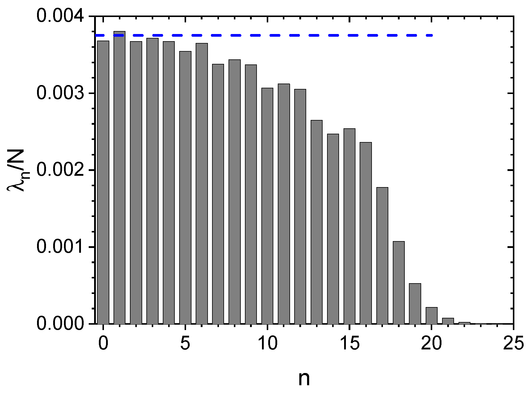
Figure 2.
for a uniform sphere with . The dashed blue line is , the dash-dotted red line is the value .
Figure 2.
for a uniform sphere with . The dashed blue line is , the dash-dotted red line is the value .

Figure 3.
(in units of ) vs. for and a uniform sphere with and , from the analytical MF solution (continuous red line), from the numerical solution of the discrete Equation (1) (dash-dot black line) and from the Timed-Dicke approximated solution, (37) (dash blue line).

Figure 4.
vs. for and a uniform sphere with and , from the analytical MF solution (continuous blue line) and from the numerical solution of the discrete Equation (1) (dashed black line). The dashed-dotted red line is the timed-Dicke approximation, , and the dotted black line is the single atom decay .

Figure 5.
for a sphere with parabolic profile, with . The dashed blue line is the value .

Figure 6.
vs. n for a sphere with Gaussian profile, with , for the exact discrete expression (40) and its continuous approximation (41) (red continuous line).

Figure 7.
(in units of ) vs. for and a Gaussian sphere with and , from the analytical MF solution (continuous red line) and from the numerical solution of the discrete Equation (1) (dashed blue line). The dotted black line is the single-atom decay as .
Figure 7.
(in units of ) vs. for and a Gaussian sphere with and , from the analytical MF solution (continuous red line) and from the numerical solution of the discrete Equation (1) (dashed blue line). The dotted black line is the single-atom decay as .

Figure 8.
(in units of ) vs. for and a Gaussian sphere with and , from the analytical MF solution (continuous red line) and from the numerical solution of the discrete Equation (1) (dashed blue line). The dotted black line is the single-atom decay, as .
Figure 8.
(in units of ) vs. for and a Gaussian sphere with and , from the analytical MF solution (continuous red line) and from the numerical solution of the discrete Equation (1) (dashed blue line). The dotted black line is the single-atom decay, as .

Figure 9.
vs. for and a Gaussian sphere with and , from the analytical MF solution (continuous red line) and from the numerical solution of the discrete Equation (22) (dashed blue line).
Figure 9.
vs. for and a Gaussian sphere with and , from the analytical MF solution (continuous red line) and from the numerical solution of the discrete Equation (22) (dashed blue line).

Disclaimer/Publisher’s Note: The statements, opinions and data contained in all publications are solely those of the individual author(s) and contributor(s) and not of MDPI and/or the editor(s). MDPI and/or the editor(s) disclaim responsibility for any injury to people or property resulting from any ideas, methods, instructions or products referred to in the content. |
© 2023 by the author. Licensee MDPI, Basel, Switzerland. This article is an open access article distributed under the terms and conditions of the Creative Commons Attribution (CC BY) license (https://creativecommons.org/licenses/by/4.0/).
Share and Cite
MDPI and ACS Style
Piovella, N. Mean-Field Description of Cooperative Scattering by Atomic Clouds. Atoms 2023, 11, 101. https://doi.org/10.3390/atoms11070101
AMA Style
Piovella N. Mean-Field Description of Cooperative Scattering by Atomic Clouds. Atoms. 2023; 11(7):101. https://doi.org/10.3390/atoms11070101
Chicago/Turabian StylePiovella, Nicola. 2023. "Mean-Field Description of Cooperative Scattering by Atomic Clouds" Atoms 11, no. 7: 101. https://doi.org/10.3390/atoms11070101
Note that from the first issue of 2016, this journal uses article numbers instead of page numbers. See further details here.