Theoretical Spectra of Lanthanides for Kilonovae Events: Ho I-III, Er I-IV, Tm I-V, Yb I-VI, Lu I-VII

Abstract

The broad emission bump in the electromagnetic spectra observed following the detection of gravitational waves created during the kilonova event of the merging of two neutron stars in August 2017, named GW170817, has been linked to the heavy elements of lanthanides (Z = 57–71) and a new understanding of the creation of heavy elements in the r-process. The initial spectral emission bump has a wavelength range of 3000–7000 Å, thus covering the region of ultraviolet (UV) to optical (O) wavelengths, and is similar to those seen for lanthanides. Most lanthanides have a large number of closely lying energy levels, which introduce extensive sets of radiative transitions that often form broad regions of lines of significant strength. The current study explores these broad features through the photoabsorption spectroscopy of 25 lanthanide ions, Ho I-III, Er I-IV, Tm I-V, Yb I-VI, and Lu I-VII. With excitation only to a few orbitals beyond the ground configurations, we find that most of these ions cover a large number of bound levels with open $4f$ orbitals and produce tens to hundreds of thousands of lines that may form one or multiple broad features in the X-ray to UV, O, and infrared (IR) regions. The spectra of 25 ions are presented, indicating the presence, shapes, and wavelength regions of these features. The accuracy of the atomic data used to interpret the merger spectra is an ongoing problem. The present study aims at providing improved atomic data for the energies and transition parameters obtained using relativistic Breit–Pauli approximation implemented in the atomic structure code SUPERSTRUCTURE and predicting possible features. The present data have been benchmarked with available experimental data for the energies, transition parameters, and Ho II spectrum. The study finds that a number of ions under the present study are possible contributors to the emission bump of GW170817. All atomic data will be made available online in the NORAD-Atomic-Data database.

1. Introduction

In 2017, the LIGO and VIRGO collaborations detected the first gravitational waves generated by the merging of two neutron stars, GW170817. This was followed by the detection of electromagnetic waves, the spectrum of which showed similarity to those of the heavy elements of lanthanides (Z = 57–71) [1,2]. The observed spectrum exhibited a broad feature or an emission bump at a wavelength range of 3000–7000 Å, covering the ultraviolet (UV) to optical (O) wavelength region. The feature moved towards the infrared (IR) region during the 10 days of observation, 18–27 August 2017, indicating the effect of opacity, i.e., the absorption of the traveling radiation by the plasma medium and re-emission with some loss of energy. The detection of the electromagnetic waves has provided new scope for an understanding of how heavy elements are formed through the r-process. Heavy elements are known to be formed by neutron capture in the s(slow)-process inside a star or by a r-(rapid)-process during a supernova explosion. The spectrum gives evidence of a new means of the creation of heavy elements during the merging of two neutron stars or two black holes, or a combination of the two. The interpretation of the emission bump of GW170817 will have a considerable impact in broadening our knowledge for a more complete picture of the characteristic atomic features and of the creation of elements. Since this finding, the need for atomic data for lanthanides and other heavy elements that can be used to interpret and provide information has increased. Over the next decade, it is expected that hundreds of mergers will be detected with the full network of current and upcoming gravitational wave detectors and electromagnetic telescopes.

Lanthanides are heavy elements with a large number of electrons (Z = 57–71). They have the core ion configuration of Xe, $\left[1s^{2}2s^{2}2p^{6}3s^{2}3p^{6}4s^{2}3d^{10}4p^{2}5s^{2}5p^{6}4d^{10}\right]$. In the ground state, the outer electron of a lanthanide can be in 4f, 6s, or 5d orbitals. The configurations of lanthanides can be described as [Xe]$4f^{i}6s^{j}6p^{k}5d^l$, where i, j, k, l are various occupancy numbers. These configurations introduce extensive numbers of radiative transitions that can form broad absorption features. Although lanthanides have been under study for a long time, the focus has been both academic and industrial, largely because of the luminescence properties and intense narrow-band emission, which have a large range of applications, such as in optical amplifiers, active waveguides, and fluorescent tubes.

Since the detection of the electromagnetic spectra, studies have been carried out to interpret the broad feature and identify the heavy elements that created it. Such study includes other elements, in addition to lanthanides, that may fall within the wavelengths of the bump. However, the accuracy in the large sets of atomic data for these elements has been a longstanding problem. Theoretically, the computation of lanthanide opacities is a formidable atomic physics problem, since these atoms and ions have a large number of electrons, causing complex electron–electron correlations and relativistic effects, and open 4d- and 4f-orbitals introduce large numbers of fine structure energy levels resulting from a large Hamiltonian matrix. Among the existing past and recent calculations carried out for the atomic data, we can note the work of Kasen et al. [3], who used the Breit–Pauli intermediate coupling code AUTOSTRUCTURE, which was created from and hence has the same atomic structure methodology as SUPERSTRUCTURE. Tanaka and Hotokezaka [4] and Tanaka et al. [5] used the relativistic HULLAC code with parametric potential, and Tanaka et al. [6] and Radžiūtė et al. [7] used the Dirac–Fock code GRASP2. Fontes et al. [8] used the semi-empirical Dirac–Fock–Slater code of Cowan [9]. Using the atomic data as well as the observed spectrum, a new periodic table with the origin of the creation of elements was produced by Johnson [10]. Kobayashi et al. [11] produced another table using theoretical and observational models, which differed somewhat from that of Johnson [10]. Kobayashi et al. also stated, “Although our calculations provide opacities of a wide range of r-process elements, the detailed spectral features in the model cannot be compared with the observed spectra because our atomic data …do not have enough accuracy in the transition wavelengths”.

Among the experimental work, the energy levels of lanthanides were measured by Martin et al. [12]. These values are listed in the NIST [13] compilation table. Carlson et al. [14] computed ionization threshold energies for the ground configuration of lanthanides, which are quoted in the NIST [13] table and are particularly useful when measured data are not available.

Individual transition probabilities, theoretical and experimental, are available for a limited number of transitions. They have been evaluated and compiled by NIST [13]. For the five lanthanides studied here, these values were obtained mainly by Meggers et al. [15], Morton [16], Komarovski [17], Wickliffe and Lawler [18], Sugar et al. [19], Penkin and Komarovski [20], and Fedchak et al. [21]. Recently, Irvine et al. [22] used calibration-free laser-induced breakdown spectroscopy (CF-LIBS) to calculate 967 transition probabilities of 13 earth elements in a plasma environment. Obaid et al. [23] measured the spectrum of photo-fragmented Ho and found a broad feature.

We present very large sets of atomic data for the 25 ions of five lanthanides, Ho, Er, Tm, Yb, and Lu, and compare them with the measured energies, transition probabilities, and Ho spectra. We present the spectral features of all 25 lanthanide ions plotted over a wide range of wavelengths.

2. Theory

Distinct lines in a spectrum are generated mainly by radiative transitions for photo-excitation by absorption or de-excitation by the emission of photons. The present study is carried out for these transitions in lanthanides. For an element X with charge Z, the process is expressed as

$$X^{+z}+h\nu \rightleftharpoons X^{+z\ast }$$

(1)

The transitions can be of several types depending on the selection rules, such as dipole allowed (E1), with the same and different spins of the initial and final states, or forbidden for lower magnitudes than those of E1; these follow different selection rules. The selection rules are determined by the angular part of the probability integral of the transition per unit time, $P_{ij}$, between two levels, i and j (e.g., [24]).

$$P_{ij}=2\pi \frac{c^2}{h^2{\nu }_{ji}^2}|<j|\frac{e}{mc}\widehat{\mathbf{e}}.\mathbf{p}{e}^{i\mathbf{k}.\mathbf{r}}{|i>|}^2\rho \left({\nu }_{ji}\right).$$

(2)

where $\mathbf{p}$ and $\mathbf{k}$ are the momenta of the electron and the photon, respectively; ${\nu }_{ij}$ is the frequency of the photon; and $\rho$ is the density of the radiation field. Various terms in $e^{i\mathbf{k}.\mathbf{r}}$ yield various multipole transitions. The first term gives the electric dipole transitions E1, the second term the electric quadrupole E2 and magnetic dipole M1, the third term the electric octupole E3 and magnetic quadrupole M2 transition, etc. Various transition parameters, such as the line strength (S), oscillator strength (f), and radiative decay rate (A), can be derived from the probability $P_{ij}$.

The transition matrix element with the first term of the expansion of Equation (2), for the E1 transition, can be written as $<{\Psi }_{B_j}\left|\right|\mathbf{D}\left|\right|{\Psi }_{B_i}>$, where $\mathbf{D}={\sum }_i{\mathbf{r}}_i$ is the dipole operator and i indicates the number of electrons in the ion; ${\Psi }_{B_i}$ and ${\Psi }_{B_j}$ are the initial and final bound levels. The generalized line strength can be reduced as

$$S={\left|〈{\Psi }_f|\sum _{j=1}^{N+1}{r}_j|{\Psi }_i〉\right|}^2$$

(3)

The oscillator strength ($f_{ij}$) and radiative decay rate ($A_{ji}$) for the bound-bound transition are obtained from S as

$$f_{ij}=\left[\frac{E_{ji}}{3g_i}\right]S,A_{ji}\left(se{c}^{-1}\right)=\left[0.8032\times {10}^{10}\frac{E_{ji}^3}{3g_j}\right]S$$

(4)

where $g_i$ and $g_j$ are the statistical weight factors; $E_{ij}$ is the transition energy in Ry. The photoabsorption cross-section can be obtained as

$$\sigma \left(\nu \right)=8.064\frac{E_{ij}}{3g_i}S \left[Mb\right]$$

(5)

Equation (5) is similar to that of the photoionization cross-section. While the photoionization and photoabsorption cross-sections are basically the same as both correspond to the absorption of a photon and can be seen in photoabsorption spectra, the photoionization cross-section is continuous as it depends on any photon energy beyond the ionization threshold, and the photoabsorption cross-section depends on the excitation energies of the bound and autoionizing states. Both can be plotted for spectral features. Researchers who do not use close-coupling approximation for the automatic generation of resonances in photoionization typically use distorted wave approximation for the background cross-section of photoionization and use the photoabsorption cross-sections as resonance lines over a smooth background.

A Lorentzian or Gaussian function is often multiplied with a photoabsorption line to broaden it in to order to simulate the width of a resonance in photoionization cross-sections. When an experiment is carried out, the lines are broadened by the bandwidth of the experimental beam and the detector. In such cases, the calculated lines can be convoluted with the bandwidth of the beam to simulate the observed spectrum. We present photoabsorption spectra without the broadening of lines. Ions, such as lanthanide ions, with a large number of quantum states generate many lines due to transitions among these states. They form almost a continuous curve in the cross-sections, as will be seen for most of the lanthanide ions studied here.

The present work includes E1 transitions to produce the synthetic spectrum of the ion and illustrate the spectral features. The magnitudes of the decay rates for forbidden transitions are typically several orders of magnitude lower than those of E1. However, E2, E3, M1, and M2 results are available for distribution in the NORAD-Atomic-Data database [25]. The present study considers both the bound-bound and bound-free (continuum) excitation as computed by the program SUPERSTRUCTURE (SS) [26].

Computations of the energies and transition parameters have been carried out in the relativistic Breit–Pauli approximation, where the Hamiltonian is given by (e.g., [24,26])

$$\begin{array}{c}\hfill {\mathbf{H}}_{\mathrm{BP}}={\mathbf{H}}_{\mathbf{NR}}+{\mathbf{H}}_{\mathrm{mass}}+{\mathbf{H}}_{\mathrm{Dar}}+{\mathbf{H}}_{\mathrm{so}}+\end{array}$$

$$\begin{array}{c}\hfill \frac{1}{2}\sum _{i\ne j}^N[g_{ij}(so+s{o}^{\prime })+g_{ij}\left(s{s}^{\prime }\right)+g_{ij}\left(cs{s}^{\prime }\right)+g_{ij}\left(d\right)+g_{ij}\left(o{o}^{\prime }\right)]\end{array}$$

(6)

where the non-relativistic Hamiltonian is given by

$$H_{NR}=\left[\sum _{i=1}^N\left\{-{\nabla }_i^2-\frac{2Z}{r_i}+\sum _{j>i}^N\frac{2}{r_{ij}}\right\}\right]$$

(7)

and the one-body mass correction, Darwin, and spin-orbit interaction terms are, respectively,

$${\displaystyle H_{mass}=-\frac{{\alpha }^2}{4}\sum _i{p}_i^4,H_{Dar}=\frac{{\alpha }^2}{4}\sum _i{\nabla }^2\left(\frac{Z}{r_i}\right),H_{so}=\frac{Z{e}^2{\hslash }^2}{2m^2{c}^2{r}^3}\mathbf{L}.\mathbf{S}}$$

(8)

while the two-body Breit interaction term is

$$H_B=\sum _{i>j}[g_{ij}(so+s{o}^{\prime })+g_{ij}\left(s{s}^{\prime }\right)]$$

(9)

The present approximation includes the contributions of all these terms and part of the last three terms of ${\mathrm{H}}_{BP}$ incorporated in the atomic structure code SS [26,27]. The prime notation for spin and orbital angular momenta in the two-body interaction terms indicates the quantity belonging to the other electron.

The electron–electron interaction, as implemented in the atomic structure program SUPERSTRUCTURE [24,26,27], is represented by the Thomas–Fermi–Dirac–Amaldi (TFDA) potential, which includes the electron exchange effect and configuration interactions. Electrons are treated as a Fermi sea of electrons, constrained by the Pauli exclusion principle, filling in cells up to the highest Fermi level of momentum $p=p_{\mathrm{F}}$ at temperature T = 0. As T rises, electrons are excited out of the Fermi sea close to the ‘surface’ level and approach a Maxwellian distribution. Solutions of the Schrodinger equation provide the wavefunctions and energies of the fine structure levels. Based on quantum statistics, the TFDA model gives a continuous function $\varphi \left(x\right)$ such that the potential is represented by [27,28]

$$V\left(r\right)=\frac{{\mathcal{Z}}_{\mathrm{eff}}({\lambda }_{nl},r)}{r}=-\frac{Z}{r}\varphi \left(x\right),$$

(10)

where

$$\varphi \left(x\right)={\mathrm{e}}^{-Zr/2}+{\lambda }_{nl}(1-{\mathrm{e}}^{-Zr/2}),x=\frac{r}{\mu },\mu =0.8853{\left(\frac{N}{N-1}\right)}^{2/3}{Z}^{-1/3}=constant.$$

(11)

${\lambda }_{nl}$ is the Thomas–Fermi scaling parameter of the $nl$ orbital wavefunction. Depending on its value, typically around 1 and less than 2, the orbital wavefunction can be compressed towards the nucleus or extended outwards. The function $\varphi \left(x\right)$ is a solution of the potential equation

$$\frac{d^2\varphi \left(x\right)}{d{x}^2}=\frac{1}{\sqrt{x}}\varphi {\left(x\right)}^{\frac{3}{2}}$$

(12)

The boundary conditions on $\varphi \left(x\right)$ are such that

$$\varphi \left(0\right)=1,\varphi (\infty )=-\frac{Z-N+1}{Z}.$$

(13)

The atomic wavefunction may be obtained by using an exponentially decaying function appropriate for a bound state, e.g., the Whittaker function.

3. Computation

As mentioned above in the Theory section, the transition parameters f, A, and photoabsorption cross-sections $\sigma$ were obtained using the atomic structure program SUPERSTRUCTURE (SS [26,27]). The wavefunction of each atomic species of the 25 lanthanide ions was optimized with a set of configurations and a set of Thomas–Fermi scaling parameters ${\lambda }_{nl}$ for the orbitals. Both sets for each ion are presented in

Table 1. Sets of optimized configurations with identifying number within parentheses and Thomas–Fermi orbital scaling parameters (${\lambda }_{\mathit{nl}}$) used in SS to compute the energies and transition parameters. All listed configurations correspond to nine inner closed or filled orbitals, $\left[1s^{2}2s^{2}2p^{6}3s^{2}3p^{6}4s^{2}3d^{10}4p^{2}5s^2\right]$, plus additional ones depending on the ion being studied. $N_T$ is the total number of transitions, allowed and forbidden, computed for each ion.

	Ho I (11 orbitals filled),  ${\mathit{N}}_{\mathit{T}}$ = 1,019,566
Configurations:	$4f^{11}6s^2$(1), $4f^{10}6s^{2}5d$(2), $4f^{10}6s^{2}6p$(3)
${\lambda }_{nl}$	1.30 (1s), 1.25 (2s), 1.12 (2p), 1.07 (3s), 1.05 (3p), 1.0 (3d), 1.0 (4s), 1.0 (4p),
	1.0 (5s), 1.60 (5p), 0.90 (4d), 0.99 (4f), 1.1 (6s), 1.1 (6p), 1.2 (5d)
	Ho II (10 orbitals filled), ${\mathit{N}}_{\mathit{T}}$ = 408,070
Configurations:	$4d^{10}4f^{11}6s$(1), $4d^{9}4f^{12}6s$(2), $4d^{10}4f^{11}6p$(3), $4d^{10}4f^{11}5d$(4)
${\lambda }_{nl}$	1.30 (1s), 1.25 (2s), 1.12 (2p), 1.07 (3s), 1.05 (3p), 1.00 (3d), 1.0 (4s), 1.0 (4p),
	1.0 (5s), 1.00 (5p), 1.0 (4d), 1.0 (4f), 1.0 (6s), 1.0 (6p), 1.0 (5d)
	Ho III (11 orbitals filled), ${\mathit{N}}_{\mathit{T}}$ = 1,309,895
Configurations:	$4f^{11}$(1), $4f^{10}5d$(2), $4f^{10}6s$(3), $4f^{10}6p$(4)
${\lambda }_{nl}$	1.30 (1s), 1.25 (2s), 1.12 (2p), 1.07 (3s), 1.05 (3p), 1.00 (3d), 1.0 (4s), 1.0 (4p),
	1.2 (5s), 0.925 (4d), 1.50 (5p), 1.00 (4f), 0.95 (6s), 1.20 (6p), 1.25 (5d)
	Er I (11 orbitals filled), ${\mathit{N}}_{\mathit{T}}$ = 206,202
Configurations:	$4f^{12}6s^2$(1), $4f^{11}6s^{2}5d$(2), $4f^{11}6s^{2}6p$(3), $4f^{12}6s6p$(4), $4f^{12}6s5d$(5)
${\lambda }_{nl}$	1.30 (1s), 1.25 (2s), 1.12 (2p), 1.07 (3s), 1.05 (3p), 1.00 (3d), 1.0 (4s), 1.05 (4p),
	1.0 (5s), 1.0 (5p), 1.0 (4d), 1.0 (4f), 1.05 (6s), 1.09 (6p), 1.0 (5d)
Configurations:	$4f^{12}6s$(1), $4f^{11}6s^2$(2), $4f^{11}6s5d$(3), $4f^{12}6p$(4), $4f^{12}5d$(5), $4f^{11}6s6p$(6)
${\lambda }_{nl}$	1.30 (1s), 1.25 (2s), 1.12 (2p), 1.07 (3s), 1.05 (3p), 1.00 (3d), 1.0 (4s), 1.0 (4p),
	1.2 (5s), 0.955 (5p), 1.02 (4d), 1.0 (4f), 1.0 (6s), 1.0 (6p), 1.0 (5d)
	Er III (9 orbitals filled), ${\mathit{N}}_{\mathit{T}}$ = 409,161
Configurations:	$4d^{10}5p^{6}4f^{12}$(1), $4d^{10}5p^{6}4f^{11}5d$(2), $4d^{10}5p^{6}4f^{11}6s$(3), $4d^{10}5p^{6}4f^{11}6p$(4),
	$4d^{10}5p^{5}4f^{12}6s$(5), $4d^{10}5p^{5}4f^{13}$(6), $4d^{10}5p^{6}4f^{10}6s^2$(7), $4d^{9}5p^{6}4f^{13}$(8)
${\lambda }_{nl}$	1.30 (1s), 1.25 (2s), 1.12 (2p), 1.07 (3s), 1.05 (3p), 1.00 (3d), 1.0 (4s), 1.0 (4p),
	1.8 (5s), 1.17 (4d), 1.01 (5p), 1.0 (4f), 1.2 (6s), 1.0 (6p), 1.0 (5d)
	Er IV (11 orbitals filled), ${\mathit{N}}_{\mathit{T}}$ = 1,309,955
Configurations:	$4f^{11}$(1), $4f^{10}5d$(2), $4f^{10}6s$(3), $4f^{10}6p$(4)
${\lambda }_{nl}$	1.30 (1s), 1.25 (2s), 1.12 (2p), 1.07 (3s), 1.05 (3p), 1.0 (3d), 1.0 (4s), 1.0 (4p), 1.0 (5s),
	1.07 (4d), 1.0 (5p), 1.0 (4f), 1.0 (5d), 1.0 (6s), 1.0 (6p)
	Tm I (11 orbitals filled), ${\mathit{N}}_{\mathit{T}}$ = 118,759
Configurations:	$4f^{13}6s^2$(1), $4f^{12}6s^{2}5d$(2), $4f^{13}6s5d$(3), $4f^{13}6s6p$(4), $4f^{12}6s^{2}6p$(5), $4f^{13}6p5d$(6),
	$4f^{13}6p^2$(7), $4f^{13}5d^2$(8), $4f^{14}6s$(9), $4f^{14}6p$(10), $4f^{14}5d$(11)
${\lambda }_{nl}$	1.30 (1s), 1.25 (2s), 1.22 (2p), 1.1 (3s), 1.12 (3p), 1.1262 (3d), 1.002 (4s), 1.0606 (4p),
	0.9 (5s), 1.05436 (5p), 0.97512 (4d), 1.0 (4f), 0.712 (6s), 1.16173 (6p), 1.096 (5d)
	Tm II (11 orbitals filled), ${\mathit{N}}_{\mathit{T}}$ = 34,184
Configurations:	$4f^{13}6s$(1), $4f^{12}6s^2$(2), $4f^{12}6s5d$(3), $4f^{13}5d$(4), $4f^{13}6p$(5), $4f^{12}5d^2$(6),
	$4f^{12}6s6p$(7), $4f^{12}6s5d$(8), $4f^{14}$(9)
${\lambda }_{nl}$	1.30 (1s), 1.25 (2s), 1.12 (2p), 1.07 (3s), 1.05 (3p), 1.01 (3d), 0.92 (4s), 0.80 (4p),
	1.53 (5s), 0.9 (5p), 1.004 (4d), 1.02 (4f), 1.014 (6s), 0.9 (6p), 0.95 (5d)
	Tm III (11 orbitals filled), ${\mathit{N}}_{\mathit{T}}$ = 849,878
Configurations:	$4f^{13}$(1), $4f^{12}5d$(2), $4f^{12}6s$(3), $4f^{12}6p$(4), $4f^{11}6s5d$(5), $4f^{11}6s6p$(6)
${\lambda }_{nl}$	1.30 (1s), 1.25 (2s), 1.12 (2p), 1.07 (3s), 1.05 (3p), 1.0 (3d), 1.0 (4s), 1.0 (4p), 1.0 (5s),
	1.12 (5p), 1.0  (4d), 0.97 (4f), 0.98 (6s),1.0 (6p), 0.98 (5d)
	Tm IV (10 orbitals filled), ${\mathit{N}}_{\mathit{T}}$ = 1,096,164
Configurations:	$5p^{6}4f^{12}$(1), $5p^{6}4f^{11}5d$(2), $5p^{6}4f^{11}6s$(3), $5p^{6}4f^{11}6p$(4), $5p^{5}4f^{13}$(5), $5p^{5}4f^{12}5d$(6),
	$5p^{5}4f^{12}6s$(7), $5p^{6}4f^{10}6s^2$(8)
${\lambda }_{nl}$	1.30 (1s), 1.25 (2s), 1.12 (2p), 1.07 (3s), 1.05 (3p), 1.0 (3d), 1.0 (4s), 1.0 (4p), 1.0 (5s),
	1.0 (4d), 1.03 (5p), 1.0 (4f), 1.0 (6s), 1.0 (6p), 1.0 (5d)
	Tm V (11 orbitals filled), ${\mathit{N}}_{\mathit{T}}$ = 801,717
Configurations:	$4f^{11}$(1), $4f^{10}5d$(2), $4f^{10}6s$(3), $4f^{10}6p$(4)
${\lambda }_{nl}$	1.3 (1s), 1.25 (2s), 1.12 (2p), 1.07 (3s), 1.05 (3p), 1.0 (3d), 1.0 (4s), 1.0 (4p), 1.0 (5s),
	1.0 (4d), 1.0 (5p), 1.0 (4f),1.0 (6s), 1.0 (6p), 1.0 (5d)
	Yb I (11 orbitals filled), ${\mathit{N}}_{\mathit{T}}$ = 109,127
Configurations:	$4f^{14}6s^2$(1), $4f^{14}6s6p$(2), $4f^{13}6s^{2}5d$(3), $4f^{14}6s5d$(4), $4f^{13}6s^{2}6p$(5), $4f^{13}6s5d^2$(6),
	$4f^{13}6s6p5d$(7), $4f^{14}6p^2$(8), $4f^{14}6p5d$(9), $4f^{14}5d^2$(10)
${\lambda }_{nl}$	1.30 (1s), 1.25 (2s), 1.12 (2p), 1.07 (3s), 1.05 (3p), 1.03 (3d), 1.05 (4s), 1.02 (4p),
	0.935 (5s), 0.937 (5p), 1.0 (4d), 1.0 (4f), 1.0 (6s), 1.0 (6p), 1.0 (5d)
	Yb II (11 orbitals filled), ${\mathit{N}}_{\mathit{T}}$ =39,009
Configurations:	$4f^{14}6s$(1), $4f^{13}6s^2$(2), $4f^{14}5d$(3), $4f^{13}6s5d$(4), $4f^{14}6p$(5), $4f^{13}5d^2$(6), $4f^{13}6s6p$(7),
	$4f^{13}6p5d$(8)
${\lambda }_{nl}$	1.30 (1s), 1.45 (2s), 1.20 (2p), 1.10 (3s), 1.07 (3p), 1.0 (3d), 1.0 (4s), 1.05 (4p),
	0.918 (5s), 0.90  (5p), 1.025 (4d), 1.0 (4f), 1.1007 (6s), 0.97 (6p), 0.97 (5d)
	Yb III (11 orbitals filled), ${\mathit{N}}_{\mathit{T}}$ = 925,575
Configurations:	$4f^{14}$(1), $4f^{13}5d$(2), $4f^{13}6s$(3), $4f^{13}6p$(4), $4f^{12}5d^2$(5), $4f^{12}6s5d$(6), $4f^{12}6p5d$(7),
	$4f^{12}6s6p$(8), $4f^{12}6s^2$(9)
${\lambda }_{nl}$	1.30 (1s), 1.25 (2s), 1.12 (2p), 1.07 (3s), 1.05 (3p), 1.15 (3d), 1.05 (4s), 0.819 (4p),
	1.24 (5s), 0.887 (5p), 0.98 (4d), 1.02 (4f), 1.05 (6s), 0.95 (6p), 1.0 (5d)
	Yb IV (10 orbitals filled), ${\mathit{N}}_{\mathit{T}}$ = 400,325
Configurations:	$4d^{10}4f^{13}$(1), $4d^{10}4f^{12}5d$(2), $4d^{10}4f^{12}6s$(3), $4d^{10}4f^{12}6p$(4), $4d^{9}4f^{14}$(5), $4d^{10}4f^{11}6s5d$(6)
${\lambda }_{nl}$	1.3 (1s), 1.25 (2s), 1.12 (2p), 1.07 (3s), 1.05 (3p), 1.0 (3d), 1.0 (4s), 1.0 (4p),
	1.0 (5s), 0.995 (5p), 1.0 (4d), 1.0 (4f), 1.0 (6s), 1.0 (6p), 1.0 (5d)
Configurations:	$4f^{12}5p^6$(1), $4f^{13}5p^5$(2), $4f^{11}5p^{6}5d$(3), $4f^{12}5p^{5}6s$(4), $4f^{11}5p^{6}6s$(5), $4f^{11}5p^{6}6p$(6)
${\lambda }_{nl}$	1.30 (1s), 1.25 (2s), 1.12 (2p), 1.07 (3s), 1.05 (3p), 1.0 (3d), 1.0 (4s), 1.0 (4p), 1.0 (5s),
	1.0 (4d), 1.03 (5p), 1.0 (4f), 1.0 (6s), 1.15 (6p), 1.2 (5d)
	Yb VI (10 orbitals filled), ${\mathit{N}}_{\mathit{T}}$ = 486,262
Configurations:	$45p^{5}4f^{12}$(1), $5p^{6}4f^{10}5d$(2), $5p^{4}4f^{12}6s$(3), $5p^{4}4f^{13}$(4)
${\lambda }_{nl}$	1.30 (1s), 1.25 (2s), 1.12 (2p), 1.07 (3s), 1.05 (3p), 1.0 (3d), 1.0 (4s), 1.0 (4p), 1.1 (5s),
	1.0 (4d), 1.0 (5p), 1.0 (4f), 1.0 (6s), 1.0 (6p), 1.0 5d
	Lu-I (12 orbitals filled), ${\mathit{N}}_{\mathit{T}}$ = 13,936
Configurations:	$5d6s^2$(1), $6s^{2}6p$(2), $5d6s6p$(3), $6s5d^2$(4), $6s6p^2$(5), $6p5d^2$(6), $5d6p^2$(7), $5p^3$(8), $5d^3$(9)
${\lambda }_{nl}$	1.30 (1s), 1.25 (2s), 1.12 (2p), 1.07 (3s), 1.05 (3p), 1.0 (3d), 1.0 (4s), 1.0 (4p),
	0.95 (5s), 1.135 (4d), 0.94 (5p), 1.0 (4f), 1.0 (6s), 0.98 (6p), 1.0 5d
	Lu-II (11 orbitals filled), ${\mathit{N}}_{\mathit{T}}$ = 109,566
Configurations:	$4f^{14}6s^2$(1), $4f^{14}6s5d$(2), $4f^{14}6s6p$(3), $4f^{14}5d^2$(4), $4f^{14}5d6p$(5), $4f^{14}6p^2$(6), $4f^{13}6s5d^2$(7),
	$4f^{13}6s^{2}5d$(8), $4f^{13}6s5d6p$(9), $4f^{13}6s^{2}6p$(10)
${\lambda }_{nl}$	1.30 (1s), 1.25 (2s), 1.12 (2p), 1.07 (3s), 1.05 (3p), 1.0 (3d), 1.0 (4s), 1.0 (4p), 0.95 (5s),
	0.937 (5p), 1.0 (4d), 1.0 (4f), 1.0 (6s), 1.0 (6p), 0.99 5d
	Lu-III (11 orbitals filled), ${\mathit{N}}_{\mathit{T}}$ = 8564
Configurations:	$4f^{14}6s$(1), $4f^{14}5d$(2), $4f^{14}6p$(3), $4f^{13}5d^2$(4), $4f^{13}5d6s$(5), $4f^{13}6s^2$(6), $4f^{13}6p5d$(7),
	$4f^{13}6s6p$(8)
${\lambda }_{nl}$	1.30 (1s), 1.25 (2s), 1.12 (2p), 1.07 (3s), 1.05 (3p), 1.00 (3d), 1.0 (4s), 1.05 (4p),
	1.0 (5s), 0.95 (5p), 0.98 (4d), 1.0 (4f), 1.03 (6s), 0.97 (6p), 0.98 5d
	Lu-IV (11 orbitals filled), ${\mathit{N}}_{\mathit{T}}$ = 926,436
Configurations:	$4f^{14}$(1), $4f^{13}5d$(2), $4f^{13}6s$(3), $4f^{13}6p$(4), $4f^{12}5d^2$(5), $4f^{12}5d6s$(6), $4f^{12}6s^2$(7),
	$4f^{12}6s6p$(8), $4f^{12}6p5d$(9)
${\lambda }_{nl}$	1.30 (1s), 1.25 (2s), 1.12 (2p), 1.07 (3s), 1.05 (3p), 1.00 (3d), 1.0 (4s), 0.80 (4p),
	1.40 (5s), 0.90 (5p), 0.98 (4d), 1.02 (4f), 1.05 (6s), 0.92 (6p), 0.97 5d
	Lu-V (11 orbitals filled), ${\mathit{N}}_{\mathit{T}}$ = 850,668
Configurations:	$4f^{13}$(1), $4f^{12}5d$(2), $4f^{12}6s$(3), $4f^{12}6p$(4), $4f^{11}5d6s$(5), $4f^{11}6s6p$(6)
${\lambda }_{nl}$	1.30 (1s), 1.25 (2s), 1.12 (2p), 1.07 (3s), 1.05 (3p), 1.0 (3d), 1.0 (4s), 1.0 (4p),
	1.0 (5s), 0.999 (5p), 0.993 (4d), 1.01 (4f), 0.98 (6s), 1.02 (6p), 1.0 5d
	Lu-VI (10 orbitals filled), ${\mathit{N}}_{\mathit{T}}$ = 317,817
Configurations:	$4f^{12}5p^6$(1), $4f^{13}5p^5$(2), $4f^{11}5p^{6}5d$(3), $4f^{12}5p^{5}6s$(4), $4f^{11}5p^{6}6s$(5), $4f^{11}5p^{6}6p$(6)
${\lambda }_{nl}$	1.30 (1s), 1.25 (2s), 1.12 (2p), 1.07 (3s), 1.05 (3p), 0.80 (3d), 1.0 (4s), 1.0 (4p),
	1.4 (5s), 0.98 (4d), 1.0 (5p), 1.0 (4f), 0.95 (6s), 1.3 (6p), 1.3 5d
	Lu-VII (10 orbitals filled), ${\mathit{N}}_{\mathit{T}}$ = 304,178
Configurations:	$4f^{13}5p^4$(1), $4f^{12}5p^5$(2), $4f^{14}5p^3$(3), $4f^{13}5p^{3}5d$(4), $4f^{13}5p^{3}6s$(5), $4f^{13}5p^{3}6p$(6)
${\lambda }_{nl}$	1.30 (1s), 1.25 (2s), 1.12 (2p), 1.07 (3s), 1.05 (3p), 1.0 (3d), 1.0 (4s), 1.0 (4p),
	1.0 (5s), 0.98 (4d), 0.97 (5p), 1.0 (4f), 1.0 (6s), 1.0 (6p), 1.12 5d

.

The optimization process for the energies was considerably complex due to the sensitivity of the potential with a large number of electrons. A large number of angular quantum numbers due to a large number of electrons with open orbitals 4f, 5p, 5d, 6s, 6p, particularly 4f, introduces a very large number of energy levels. Hence, a slight variation in the Thomas–Fermi scaling parameters ${\lambda }_{nl}$ for the orbital wavefunctions would perturb the electron–electron interaction and change the energy values and the order in the fine structure levels. A numerical challenge arose when exceeding the dimension of the Hamiltonian matrix that SS can accommodate. The number of digital spaces for the dimension surpassed those allotted to SS. Hence, the optimization of the set of configurations was carried out carefully such that the order of the calculated energy levels, particularly the ground and low-lying energies, could match to those of the measured energies available in the NIST [13] table.

Table 1 presents the optimized set of configurations, specifying the occupancy of the outer orbitals that can vary while specifying the number of inner orbitals that remain closed, as well as the Thomas–Fermi scaling parameters of the orbitals for each ion. The top line of each set gives the total number of radiative transitions ($N_T$), which includes both the allowed E1 and forbidden E2, E3, M1, M2 transitions, produced by a set of configurations.

All atomic data from SS were processed using the program PRCSS [29] to obtain clean tables and easy applications of them. They were further processed to compute absorption cross-sections, sum them if the transition energies were the same, and display the spectral features using the program SPECTRUM [30].

4. Results and Discussion

The present study reports results on the energies and transitions and corresponding photoabsorption spectra of 25 ions of lanthanides, Ho I-III, Er I-IV, Tm I-V, Yb I-VI, and Lu I-VII. We investigate the spectral features of these ions. Most of the ions have produced close to hundreds of thousands lines, with excitation to a few orbitals upwards. All atomic data for all 25 lanthanides ions considered in the present study are available in the NORAD-Atomic-Data database [25].

The present results correspond to a limited number of configurations for each ion. For most ions, configurations with orbitals up to 6p, 5d are only considered; for some ions, such as Ho I, no additional configurations beyond those already included could be considered due to exceeding the limit on the dimensions of various arrays, such as that of the Hamiltonian matrix, in the program. These issues are mentioned in the Computation section. For some other ions, it was possible to add more configurations, but they were omitted at the end, as they produced energies that were much higher than and had an energy gap with the lower levels. It was not possible to verify the accuracy of these high-lying energies due to the lack of availability of observed energies. These configurations also introduced additional electron–electron correlation interactions, which impacted the order and numerical values of the lower energies. This implies that significantly more configurations would be needed for a converged and larger set of accurate energies. Thus, we selected the set of configurations that provided the overall best set of energies when compared to those available at NIST for each ion.

It was observed that these large ions do not show the isoelectronic behavior that is often seen with lower Z elements. Hence, the isoelectronic set of large ions does not necessarily have the same set of optimized configurations. The energy tables of the present lanthanide ions available in the NIST table confirm this behavior, namely that these ions may not have the same symmetries for the ground and low-lying levels. The photoabsorption features of the isoelectronic series, such as Ho I, Er II, Tm III, Yb IV, and Lu V, as will be seen later, do not have similar features.

We discuss some general information and data files for the 25 ions, before giving examples of the characteristics of individual ions.

4.1. General Information on the Atomic Data

Each lanthanide ion produced a significantly large number of energy levels. A file containing all energies for each ion, as mentioned above, is available electronically in the NORAD-Atomic-Data database [25]. A sample set of energies for Ho I is presented in

Table 2. Sample table of energies for Ho I demonstrating the format of the complete energy table for each lanthanide ion. The total number of levels obtained is given at the top. The column headings are as follows: ie is the running index, $SL\pi$(C#) is the symmetry (total spin S, total orbital angular momentum L, and parity $\pi$), $cf\#$ is the configuration number as given in Table 1, J is the total angular momentum, and E is the relative energy in Ry.

Number of Fine Structure Levels = 1629ie	SL$\mathbf{\pi }$(cf#)	J	E(Ry)
1	4Io(1)	15/2	0.00000E+00
2	4Io(1)	13/2	3.60033E-02
3	4Io(1)	11/2	5.85101E-02
4	4Io(1)	9/2	7.43454E-02
5	4Me(2)	15/2	9.79376E-02
6	6Le(2)	13/2	1.01223E-01
7	4Fo(1)	9/2	1.09269E-01
8	6Le(2)	11/2	1.22576E-01
9	2Ho(1)	11/2	1.28064E-01
10	4So(1)	3/2	1.35965E-01

to demonstrate the format of the complete energy table of the ions. In Table 2, the number of energy levels obtained from the set of configurations (Table 1) is quoted at the top of Table 2. The total number may include both the bound levels below the ionization threshold and the Rydberg levels in continuum above it.

Table 2 contains, for each energy level, the running index (ie), the symmetry of the level $SL\pi (C\#)$ with the configuration number $(C\#)$ from Table 1 within parentheses next to it, the total angular momenta J, and the energy in Ry relative to the ground level. In an atomic structure calculation, such as the present case with SS, all energies are computed relative to the ground level, which is set to zero. Hence, all energies presented are positive. The program SS does not distinguish between the bound and continuum levels. This is the same format that is followed by NIST [13], which also presents relative energies to the ground level. However, NIST provides the ionization threshold energy, which is obtained separately. The present energies are compared in

Table 3. Ground and low-lying excited energy levels of Ho, Er, Tm, Yb, Lu ions obtained from SUPERSTRUCTURE (SS) are presented and compared with measured values, largely obtained by Martin et al. [12], available in the compiled table of NIST [13]. Each configuration below corresponds to electrons outside the core ion configuration of Xe and filled $4d$ orbitals unless 4d has vacancies. $N_E$ is the number of energy levels and $N_{E1}$ is the number of corresponding E1 transitions obtained from the configuration set of each ion.

	Config	SL$\mathit{\pi }$	J	E(SS, Ry)	E(NIST [12], Ry)
Ho I, $N_E$ = 1629, $N_{E1}$ = 210,522
1	$4f^{11}6s^2$	${ }^4{I}^o$	15/2	0.0	0.0
2	$4f^{11}6s^2$	${ }^4{I}^o$	13/2	0.03603	0.0493879
3	$4f^{11}6s^2$	${ }^4{I}^o$	11/2	0.05851	0.0784160
4	$4f^{11}6s^2$	${ }^4{I}^o$	9/2	0.07434	0.0974668
5	$4f^{11}6s^2$	${ }^{4}M$	17/2	0.13881	0.0763542
6	$4f^{10}5d6s^2$	${ }^{4}M$	15/2	0.09794	0.0767935
7	$4f^{10}5d6s^2$	${ }^{6}L$	13/2	0.10122	0.0833543
8	$4f^{10}5d6s^2$	${ }^{6}L$	19/2	0.19610	0.0887711
9	$4f^{11}6s^2$	${ }^4{F}^o$	9/2	0.10927	0.1193261
10	$4f^{10}5d6s^2$	${ }^{6}L$	11/2	0.12257	0.1543452
Ho II, $N_E$ = 924, $N_{E1}$ = 81,623
1	$4f^{11}6s$	${ }^5{I}^o$	8	0.0	0.0
2	$4f^{11}6s$	${ }^5{I}^o$	7	0.00724	0.005808
3	$4f^{11}6s$	${ }^3{I}^o$	7	0.05528	0.051186
4	$4f^{11}6s$	${ }^5{I}^o$	6	0.05793	0.053306
5	$4f^{11}6s$	${ }^5{I}^o$	5	0.08928	0.080652
6	$4f^{11}6s$	${ }^3{I}^o$	6	0.09113	0.082029
7	$4f^{11}5d$	${ }^5{G}^o$	6	0.11003	0.098771
8	$4f^{11}6s$	${ }^5{I}^o$	4	0.11108	0.102111
9	$4f^{11}6s$	${ }^3{I}^o$	9	0.11702	0.148388
10	$4f^{11}5d$	${ }^5{H}^o$	7	0.11832	0.152628
Ho III, $N_E$ = 1837, $N_{E1}$ = 258,124
1	$4f^{11}$	${ }^4{I}^o$	15/2	0.0	0.0
2	$4f^{11}$	${ }^4{I}^o$	13/2	0.03114	0.04956
3	$4f^{11}$	${ }^4{I}^o$	11/2	0.04969	0.07877
4	$4f^{11}$	${ }^4{I}^o$	9/2	0.06203	0.09815
6	$4f^{11}$	${ }^4{F}^o$	9/2	0.08576	0.12147
7	$4f^{11}$	${ }^4{F}^o$	7/2	0.1149	0.16282
8	$4f^{11}$	${ }^4{F}^o$	5/2	0.1245	0.17656
9	$4f^{11}$	${ }^4{F}^o$	3/2	0.1261
10	$4f^{11}$	${ }^2{H}^o$	11/2	0.10275	0.15392
Er I. $N_E$ = 993, $N_{E1}$ = 88,827
1	$4f^{12}6s^2$	${ }^{3}H$	6	0.0	0.0
2	$4f^{12}6s^2$	${ }^{3}H$	5	0.06787	0.063408
3	$4f^{12}6s^2$	${ }^{3}H$	4	0.06158	0.097970
4	$4f^{12}6s^2$	${ }^{3}F$	4	0.11386	0.045884
5	$4f^{12}6s^2$	${ }^{3}F$	3	0.13971	0.112792
6	$4f^{12}6s^2$	${ }^{3}F$	2	0.15311	0.119357
7	$4f^{11}5d6s^2$	${ }^5{G}^o$	6	0.089544	0.065397
8	$4f^{11}5d6s^2$	${ }^5{I}^o$	7	0.097936	0.070140
9	$4f^{11}5d6s^2$	${ }^5{K}^o$	9	0.104784	0.078556
10	$4f^{11}5d6s^2$	${ }^5{I}^o$	8	0.114163	0.085204
Er II, $N_E$ = 1476, $N_{E1}$ = 189,738
1	$4f^{12}6s$	${ }^{4}H$	13/2	0.0	0.0
2	$4f^{12}6s$	${ }^{4}H$	11/2	0.06837	0.0661522
3	$4f^{12}6s$	${ }^{2}H$	9/2	0.06211	0.046772
4	$4f^{12}6s$	${ }^{4}H$	7/2	0.06260	0.049242
5	$4f^{11}6s^2$	${ }^4{I}^o$	15/2	0.18768	0.062192
6	$4f^{11}6s^2$	${ }^4{I}^o$	13/2	0.24412	0.121552
7	$4f^{11}6s^2$	${ }^4{I}^o$	11/2	0.28125	0.154443
8	$4f^{12}6s$	${ }^{2}I$	11/2	0.36487	0.065153
9	$4f^{12}6s$	${ }^{4}F$	9/2	0.11218	0.065567
10	$4f^{11}5d6s$	${ }^6{L}^o$	13/2	0.09742	0.097206
Er III, $N_E$ = 1000, $N_{E1}$ = 82,286
1	$4f^{12}$	${ }^{3}H$	6	0.0	0.0
2	$4f^{12}$	${ }^{3}H$	5	0.045163	0.063513
3	$4f^{12}$	${ }^{3}H$	4	0.035074	0.098284
4	$4f^{12}$	${ }^{3}F$	2	0.09552
5	$4f^{12}$	${ }^{3}F$	3	0.08826
6	$4f^{12}$	${ }^{3}F$	4	0.07184	0.04631
7	$4f^{11}5d$	${ }^5{G}^o$	6	0.10297	0.15469
8	$4f^{11}5d$	${ }^5{H}^o$	7	0.10991	0.160818
9	$4f^{11}5d$	${ }^5{K}^o$	9	0.14872	0.172929
10	$4f^{11}5d$	${ }^5{L}^o$	8	0.13645	0.181508
Er IV, $N_E$ = 1837, $N_{E1}$ = 257,713
1	$4f^{11}$	${ }^4{I}^o$	15/2	0.0	0.0
2	$4f^{11}$	${ }^4{I}^o$	13/2	0.0598	0.0591
3	$4f^{11}$	${ }^4{I}^o$	11/2	0.0970	0.0921
4	$4f^{11}$	${ }^4{I}^o$	9/2	0.1230	0.1125
5	$4f^{11}$	${ }^4{F}^o$	9/2	0.1770	0.1383
6	$4f^{11}$	${ }^4{F}^o$	7/2	0.2333	0.1863
7	$4f^{11}$	${ }^4{F}^o$	5/2	0.2525	0.2011
8	$4f^{11}$	${ }^4{F}^o$	3/2	0.2555	0.2042
9	$4f^{11}$	${ }^2{H}^o$	11/2	0.2103
10	$4f^{11}$	${ }^4{S}^o$	3/2	0.2193	0.1667
Tm I, $N_E$ = 470, $N_{E1}$ = 23,804
1	$4f^{13}6s^2$	${ }^2{F}^o$	7/2	0.0	0.0
2	$4f^{11}6s^2$	${ }^2{F}^o$	5/2	0.0891	0.0799
3	$4f^{12}6s^{2}5d$	${ }^{4}F$	9/2	0.1343	0.11956
4	$4f^{12}6s^{2}5d$	${ }^{2}K$	15/2	0.2030	0.1716
5	$4f^{12}6s^{2}5d$	${ }^{4}G$	11/2	0.21430	0.14205
6	$4f^{12}6s^{2}5d$	${ }^{4}K$	13/2	0.25119	0.15906
7	$4f^{12}6s^{2}5d$	${ }^{4}K$	17/2	0.31023	0.14997
8	$4f^{12}6s^{2}5d$	${ }^{4}F$	7/2	0.20683	0.15452
9	$4f^{12}6s^{2}5d$	${ }^{4}I$	15/2	0.38814	0.17034
10	$4f^{12}6s^{2}5d$	${ }^{4}G$	9/2	0.28376	0.17165
Tm II, $N_E$ = 1129, $N_{E1}$ = 2467
1	$4f^{13}6s$	${ }^3{F}^o$	4	0.0	0.0
2	$4f^{13}6s$	${ }^1{F}^o$	3	0.000309	0.00216
3	$4f^{13}6s$	${ }^3{F}^o$	2	0.1050	0.0799
4	$4f^{13}6s$	${ }^3{F}^o$	3	0.1053	0.0816
5	$4f^{12}6s^2$	${ }^{3}H$	6	0.1449	0.1135
6	$4f^{12}6s^2$	${ }^{3}H$	5	0.2272	0.1879
7	$4f^{12}6s^2$	${ }^{3}H$	4	0.1812	0.2272
8	$4f^{12}5d6s$	${ }^{5}F$	5	0.1362	0.1510
9	$4f^{12}5d6s$	${ }^{3}K$	7	0.14733	0.17878
10	$4f^{12}5d6s$	${ }^{5}G$	6	0.15250	0.2032
Tm III, $N_E$ = 1437, $N_{E1}$ = 181,768
1	$4f^{13}$	${ }^2{F}^o$	7/2	0.0	0.0
2	$4f^{13}$	${ }^2{F}^o$	5/2	0.06669	0.07995
3	$4f^{12}5d$	${ }^{4}F$	9/2	0.24034	0.20866
4	$4f^{12}5d$	${ }^{4}H$	15/2	0.27574	0.235825
5	$4f^{12}5d$	${ }^{4}H$	11/2	0.27975	0.239230
6	$4f^{12}5d$	${ }^{4}K$	13/2	0.30738	0.261724
7	$4f^{12}6s$	${ }^{2}H$	13/2	0.21097	0.230575
8	$4f^{12}6s$	${ }^{2}H$	11/2	0.21716	0.236207
9	$4f^{12}5d$	${ }^{4}H$	7/2	0.27029	0.251029
10	$4f^{12}5d$	${ }^{4}I$	17/2	0.28719	0.251127
Tm IV, $N_E$ = 1606, $N_{E1}$ = 160,013
1	$4f^{12}$	${ }^{3}H$	6	0.0	0.0
2	$4f^{12}$	${ }^{3}H$	5	0.08038	0.0737
3	$4f^{12}$	${ }^{3}H$	4	0.06591	0.114
4	$4f^{12}$	${ }^{3}F$	4	0.12865	0.0514
5	$4f^{12}$	${ }^{3}F$	3	0.15760	0.1308
6	$4f^{12}$	${ }^{3}F$	2	0.17087	0.1353
7	$4f^{12}$	${ }^{1}G$	4	0.21265	0.1943
8	$4f^{12}$	${ }^{1}D$	2	0.33334
9	$4f^{12}$	${ }^{1}I$	6	0.40132
10	$4f^{12}$	${ }^{3}P$	0	0.43598
Tm V, $N_E$ = 1837, $N_{E1}$ = 259,539
1	$4f^{11}$	${ }^4{I}^o$	15/2	0.0	0.0
2	$4f^{11}$	${ }^4{I}^o$	13/2	0.04067
3	$4f^{11}$	${ }^4{I}^o$	11/2	0.06393
4	$4f^{11}$	${ }^4{I}^o$	9/2	0.07922
5	$4f^{11}$	${ }^4{F}^o$	9/2	0.10784
6	$4f^{11}$	${ }^2{H}^o$	11/2	0.12898
7	$4f^{11}$	${ }^4{S}^o$	3/2	0.13396
8	$4f^{11}$	${ }^4{F}^o$	7/2	0.14556
9	$4f^{11}$	${ }^4{F}^o$	5/2	0.15756
10	$4f^{11}$	${ }^4{F}^o$	3/2	0.15875
Yb I, $N_E$ = 455, $N_{E1}$ = 22,002
1	$4f^{14}6s^2$	${ }^{1}S$	0	0.0	0.0
2	$4f^{14}6s6p$	${ }^3{P}^o$	0	0.11722	0.157544
3	$4f^{14}6s6p$	${ }^3{P}^o$	1	0.12353	0.163955
4	$4f^{14}6s6p$	${ }^3{P}^o$	2	0.13864	0.179614
5	$4f^{13}5d6s^2$	${ }^3{H}^o$	2	0.17604	0.211309
6	$4f^{13}5d6s^2$	${ }^3{H}^o$	5	0.21229	0.235651
7	$4f^{13}5d6s^2$	${ }^3{D}^o$	3	0.23746	0.250103
8	$4f^{13}5d6s^2$	${ }^3{H}^o$	4	0.25282	0.256836
9	$4f^{14}5d6s$	${ }^{3}D$	1	0.37221	0.223161
10	$4f^{14}5d6s$	${ }^{3}D$	2	0.37380	0.225556
Yb II, $N_E$ = 264, $N_{E1}$ = 8033
1	$4f^{14}6s$	${ }^{2}S$	1/2	0.0	0.0
2	$4f^{13}6s^2$	${ }^2{F}^o$	7/2	0.12512	0.195182
3	$4f^{13}6s^2$	${ }^2{F}^o$	5/2	0.22718	0.287669
4	$4f^{14}5d$	${ }^{2}D$	3/2	0.13701	0.209234
5	$4f^{14}5d$	${ }^{2}D$	5/2	0.15567	0.221736
6	$4f^{13}6s5d$	${ }^4{P}^o$	5/2	0.20627	0.243846
7	$4f^{13}6s5d$	${ }^4{P}^o$	3/2	0.23529	0.262062
8	$4f^{13}6s5d$	${ }^4{P}^o$	1/2	0.28170	0.306676
9	$4f^{14}6s6p$	${ }^2{P}^o$	1/2	0.25680	0.246605
10	$4f^{14}6s6p$	${ }^2{P}^o$	3/2	0.27636	0.276954
Yb III, $N_E$ = 1485, $N_{E1}$ = 203,904
1	$4f^{14}$	${ }^{1}S$	0	0.0	0.0
2	$4f^{13}5d$	${ }^3{P}^o$	2	0.31312	0.304234
3	$4f^{13}5d$	${ }^3{H}^o$	5	0.35368	0.337353
4	$4f^{13}5d$	${ }^3{D}^o$	3	0.381433	0.356681
5	$4f^{13}5d$	${ }^3{H}^o$	4	0.397868	0.365965
6	$4f^{13}6s$	${ }^3{F}^o$	4	0.313955	0.315810
7	$4f^{13}6s$	${ }^1{F}^o$	3	0.314706	0.318858
8	$4f^{13}5d$	${ }^3{H}^o$	6	0.387298	0.365965
9	$4f^{13}5d$	${ }^3{P}^o$	1	0.393126	0.361962
10	$4f^{13}5d$	${ }^3{D}^o$	2	0.406379	0.367132
Yb IV, $N_E$ = 963, $N_{E1}$ = 40,767
1	$4f^{13}$	${ }^2{F}^o$	7/2	0.0	0.0
2	$4f^{13}$	${ }^2{F}^o$	5/2	0.10849	0.093077
3	$4f^{12}5d$	${ }^{4}F$	9/2	0.68093	0.715611
4	$4f^{12}5d$	${ }^{2}K$	15/2	0.71781	0.748930
5	$4f^{12}5d$	${ }^{4}G$	11/2	0.72798	0.753373
6	$4f^{12}5d$	${ }^{4}K$	13/2	0.75809	0.779549
7	$4f^{12}5d$	${ }^{4}F$	7/2	0.74697	0.768627
8	$4f^{12}5d$	${ }^{4}K$	17/2	0.75311	0.775715
9	$4f^{12}5d$	${ }^{4}G$	9/2	0.78667	0.802991
10	$4f^{12}5d$	${ }^{4}I$	11/2	0.79105	0.803512
Yb V, $N_E$ = 873, $N_{E1}$ = 59,027
1	$4f^{12}5p^6$	${ }^{3}H$	6	0.0	0.0
2	$4f^{12}5p^6$	${ }^{3}H$	4	0.031148
3	$4f^{12}5p^6$	${ }^{3}H$	5	0.056967
4	$4f^{12}5p^6$	${ }^{3}F$	4	0.085510
5	$4f^{12}5p^6$	${ }^{3}F$	3	0.10029
6	$4f^{12}5p^6$	${ }^{3}F$	2	0.10611
7	$4f^{12}5p^6$	${ }^{1}G$	4	0.13819
8	$4f^{12}5p^6$	${ }^{1}D$	2	0.21423
9	$4f^{12}5p^6$	${ }^{1}I$	6	0.26570
10	$4f^{12}5p^6$	${ }^{3}P$	0	0.28940
Yb VI, $N_E$ = 1407, $N_{E1}$ = 13,807
1	$4f^{12}5p^5$	${ }^4{I}^o$	15/2	0.0	0.0
2	$4f^{12}5p^5$	${ }^4{H}^o$	11/2	0.020645
3	$4f^{12}5p^5$	${ }^4{I}^o$	13/2	0.021470
4	$4f^{12}5p^5$	${ }^2{H}^o$	9/2	0.024775
5	$4f^{12}5p^5$	${ }^2{G}^o$	11/2	0.036494
6	$4f^{12}5p^5$	${ }^2{G}^o$	5/2	0.072901
7	$4f^{12}5p^5$	${ }^2{H}^o$	11/2	0.074037
8	$4f^{12}5p^5$	${ }^4{H}^o$	11/2	0.082992
9	$4f^{12}5p^5$	${ }^4{F}^o$	7/2	0.093051
10	$4f^{12}5p^5$	${ }^2{G}^o$	9/2	0.103729
Lu I, $N_E$ = 148, $N_{E1}$ = 3220
1	$5d6s^2$	${ }^{2}D$	3/2	0.0	0.0
2	$5d6s^2$	${ }^{2}D$	5/2	0.020658	0.018170
3	$6s^{2}6p$	${ }^2{P}^o$	1/2	0.083090	0.037691
4	$6s^{2}6p$	${ }^2{P}^o$	3/2	0.097783	0.068130
5	$5d6s6p$	${ }^4{F}^o$	3/2	0.116829	0.158809
6	$5d6s6p$	${ }^4{F}^o$	5/2	0.123975	0.168626
7	$5d6s6p$	${ }^4{F}^o$	7/2	0.137319	0.186195
8	$5d6s6p$	${ }^4{F}^o$	9/2	0.152215	0.206033
9	$5d^{2}6s$	${ }^{4}F$	3/2	0.251670	0.171785
10	$5d^{2}6s$	${ }^{4}F$	5/2	0.258495	0.176816
Lu II, $N_E$ = 455, $N_{E1}$ = 22,154
1	$6s^2$	${ }^{1}S$	0	0.0	0.0
2	$5d6s$	${ }^{3}D$	1	0.088774	0.107495
3	$5d6s$	${ }^{3}D$	2	0.098492	0.113319
4	$5d6s$	${ }^{3}D$	3	0.132393	0.129392
5	$5d6s$	${ }^{1}D$	2	0.162822	0.157946
6	$6s6p$	${ }^3{P}^o$	0	0.235055	0.248452
7	$6s6p$	${ }^3{P}^o$	1	0.248583	0.259740
8	$6s6p$	${ }^3{P}^o$	2	0.288652	0.295736
9	$5d^2$	${ }^{3}F$	2	0.286572	0.267974
10	$5d^2$	${ }^{3}F$	3	0.318543	0.281482
Lu III, $N_E$ = 145, $N_{E1}$ = 159
1	$4f^{14}6s$	${ }^{2}S$	1/2	0.0	0.0
2	$4f^{14}5d$	${ }^{2}D$	3/2	0.0510604	0.052011
3	$4f^{14}5d$	${ }^{2}D$	5/2	0.0956229	0.078805
4	$4f^{14}6p$	${ }^2{P}^o$	1/2	0.342017	0.349932
5	$4f^{14}6p$	${ }^2{P}^o$	3/2	0.379465	0.407384
6	$4f^{13}5d^2$	${ }^4{G}^o$	5/2	0.741428
7	$4f^{13}5d^2$	${ }^4{F}^o$	7/2	0.743474
8	$4f^{13}5d^2$	${ }^4{D}^o$	3/2	0.745181
9	$4f^{13}5d^2$	${ }^4{I}^o$	11/2	0.758697
10	$4f^{13}5d^2$	${ }^4{F}^o$	7/2	0.766942
Lu IV, $N_E$ = 1485, $N_{E1}$ = 204,567
1	$4f^{14}$	${ }^{1}S$	0	0.0	0.0
2	$4f^{13}5d$	${ }^3{P}^o$	2	0.860650	0.824085
3	$4f^{13}5d$	${ }^3{H}^o$	5	0.894914	0.863590
4	$4f^{13}5d$	${ }^3{D}^o$	3	0.919319	0.886969
5	$4f^{13}5d$	${ }^3{H}^o$	4	0.934682	0.898131
6	$4f^{13}5d$	${ }^3{H}^o$	6	0.927311	0.895222
7	$4f^{13}5d$	${ }^3{P}^o$	1	0.939756	0.897644
8	$4f^{13}5d$	${ }^3{P}^o$	2	0.943373	0.908169
9	$4f^{13}5d$	${ }^3{F}^o$	4	0.971074	0.931466
10	$4f^{13}5d$	${ }^3{F}^o$	3	0.971264	0.939247
Lu V, $N_E$ = 1437, $N_{E1}$ = 182,086
1	$4f^{13}$	${ }^2{F}^o$	7/2	0.0	0.0
2	$4f^{13}$	${ }^2{F}^o$	5/2	0.12751	0.107464
3	$4f^{12}5d$	${ }^{4}F$	7/2	1.45797	1.373872
4	$4f^{12}5d$	${ }^{4}F$	9/2	1.39228	1.412341
5	$4f^{12}5d$	${ }^{4}G$	9/2	1.48568	1.429373
6	$4f^{12}5d$	${ }^{4}G$	7/2	1.50702	1.448762
7	$4f^{12}5d$	${ }^{4}G$	5/2	1.50048	1.449241
8	$4f^{12}5d$	${ }^{4}F$	5/2	1.53991	1.476007
9	$4f^{12}5d$	${ }^{4}H$	7/2	1.53119	1.481346
10	$4f^{12}5d$	${ }^{4}G$	9/2	1.51306	1.483601
Lu VI, $N_E$ = 873, $N_{E1}$ = 59,028
1	$4f^{12}5p^6$	${ }^{3}H$	6	0.0	0.0
2	$4f^{12}5p^6$	${ }^{3}H$	4	0.030443
3	$4f^{12}5p^6$	${ }^{3}H$	5	0.055132
4	$4f^{12}5p^6$	${ }^{3}F$	4	0.083617
5	$4f^{12}5p^6$	${ }^{3}F$	3	0.099283
6	$4f^{12}5p^6$	${ }^{3}F$	2	0.106151
7	$4f^{12}5p^6$	${ }^{1}G$	4	0.133692
8	$4f^{12}5p^6$	${ }^{1}D$	2	0.219180
9	$4f^{12}5p^6$	${ }^{1}I$	6	0.280176
10	$4f^{12}5p^6$	${ }^{3}P$	0	0.305074
Lu VII, $N_E$ = 777, $N_{E1}$ = 68,947
1	$4f^{13}5p^4$	${ }^2{H}^o$	11/2	0.0	0.0
2	$4f^{13}5p^4$	${ }^2{H}^o$	9/2	0.0125831
3	$4f^{13}5p^4$	${ }^4{F}^o$	3/2	0.0421028
4	$4f^{13}5p^4$	${ }^4{G}^o$	7/2	0.0666561
5	$4f^{13}5p^4$	${ }^4{G}^o$	5/2	0.104410
6	$4f^{13}5p^4$	${ }^4{F}^o$	5/2	0.104410
7	$4f^{13}5p^4$	${ }^4{D}^o$	3/2	0.123075
8	$4f^{13}5p^4$	${ }^4{D}^o$	1/2	0.127465
9	$4f^{13}5p^4$	${ }^2{G}^o$	9/2	0.147603
10	$4f^{13}5p^4$	${ }^4{F}^o$	7/2	0.224123

with the measured values that are available on the NIST website.

Each lanthanide ion has produced an extensive set of transitions, including both allowed and forbidden types, among its large number of energy levels. The allowed transitions are strong. The forbidden transitions are much weaker compared to E1 transitions. We have obtained a very large set of forbidden transitions of types E2, E3, M1, and M2 for each ion. The atomic data file for each ion contains four tables of transitions: (i) a table of dipole allowed E1 transitions where the spin remains the same as the transition; (ii) a table of dipole allowed E1 transitions where the spin changes (these transitions are also known as intercombination transitions); (iii) a table of forbidden E3 and M2 transitions (they follow the same selection rules); and (iv) a table of E2 and M1 transitions (they follow the same selection rules). At the end of each table, the total number of transitions is given. The file containing the complete sets of transition parameters, i.e., the line strengths, oscillator strengths, and radiative decay rates, is available electronically from the NORAD-Atomic-Data database [25]. It is the same file that contains the energy table.

Table 4. Sample table of dipole allowed E1 transitions with same spin for Ho I to demonstrate the format of the complete table of transitions. i and j are the energy level numbers of transitional levels i and j, SLpiCi and SLpCj are the transitional level symmetries with their configuration numbers, gi and gj are the statistical weight factors (as given in the energy table), wl(A) is the wavelength of the transition in Å, fij is the oscillator strength, and aji(s-1) is the radiative decay rate in ${\sec }^{-1}$.

i-j	SLp Ci-SLp Cj	gi-gj	wl(A)	fij	aji(s-1)
29-3	4Ie  2-4Io 1	12-10	6454.84	4.24E-06	8.15E+02
29-4	4Ie  2-4Io 1	10-10	7270.34	4.48E-06	5.65E+02
42-2	4Ke  2-4Io 1	14-12	4678.36	9.76E-06	3.47E+03
42-3	4Ke  2-4Io 1	12-12	5289.56	1.11E-05	2.65E+03
42-4	4Ke  2-4Io 1	10-12	5824.98	8.06E-07	1.32E+02
…
361-455	2Po 1-2Pe 2	4-2	946.19	7.21E-02	1.07E+09

presents an example set of E1 transitions with unchanged spin belonging to Ho I, to demonstrate the format of the complete table. As explained in the caption, i and j are the transitional level numbers; $SLpCi$ is the symmetry with total spin S, total orbital angular momentum L, and parity p; $Ci$ is the configuration number of the level that it belongs to; $g_i$ is the statistical weight factor; $f_{ij}$ is the oscillator strength; and $a_{ji}$ is the radiative decay rate for the transition. The other tables for forbidden transitions are self-explanatory for the transitional quantities, as explained for Table 4. Hence, sample tables for these are not presented. The A-values from the present work are compared with the available published values in

Table 5. Comparison of A-values between the present calculated results and those available in the NIST [13] compilation table. fij is the oscillator strength and aji(s-1) is the radiative decay rate in ${\sec }^{-1}$ for transitions from level i to j.

${\mathit{A}}_{\mathit{ji}}\left({\mathit{s}}^{-1}\right)$		Transition
NIST	SS
Ho I
3.73$\times {10}^7$	2.77$\times {10}^7$	$4f^{11}6s^2{(}^4{I}_{15/2}^o)$−$4f^{10}5d6s^2{(}^4{K}_{13/2})$
1.62$\times {10}^8$	1.00$\times {10}^8$	$4f^{11}6s^2{(}^4{I}_{15/2}^o)$−$4f^{10}5d6s^2{{(}^4{I}^o)}_{15/2})$
Ho II
6.35$\times {10}^7$	3.09$\times {10}^7$	$4f^{11}6s{(}^4{I}_8^o)-4f^{11}6p{(}^4{I}_8)$
4.87$\times {10}^7$	4.64$\times {10}^7$	$4f^{11}6s{(}^4{I}_7^o)-4f^{11}6p{(}^4{I}_8)$
Ho III: No A-value is available
Er I
1.16$\times {10}^8$	2.49$\times {10}^8$	$4f^{12}6s^2{(}^3{H}_6)-4f^{12}6s6p{(}^3{H}_6^o)$
7.28$\times {10}^7$	7.26$\times {10}^7$	$4f^{12}6s^2{(}^3{H}_6)-4f^{11}5d6s^2{(}^3{I}_5^o)$
Er II
2.0$\times {10}^7$	4.67$\times {10}^7$	$4f^{12}6s{(}^4{H}_{13/2})-4f^{11}5d6s{(}^4{I}_{11/2}^o)$
1.4$\times {10}^7$	1.01$\times {10}^7$	$4f^{12}6s{(}^4{H}_{13/2})-4f^{12}6p{(}^4{I}_{13/2}^o)$
NIST	SS
Er III, Er IV: No A-value is available
Tm I
5.3$\times {10}^6$	3.33$\times {10}^6$	$4f^{13}6s^2{(}^2{F}_{7/2}^o)-4f^{12}5d6s^2{(}^2{G}_{9/2})$
1.47$\times {10}^7$	1.81$\times {10}^7$	$4f^{13}6s^2{(}^2{F}_{7/2}^o)-4f^{12}5d6s^2{(}^2{G}_{7/2})$
Tm II
1.06$\times {10}^8$	7.29$\times {10}^7$	$4f^{13}6s{(}^3{F}_4^o)-4f^{12}5d6s{(}^3{G}_5)$
1.57$\times {10}^7$	2.19$\times {10}^7$	$4f^{13}6s{(}^3{F}_4^o)-4f^{12}5d6s{(}^3{F}_4)$
Tm III, IV, V: No A-value is available
Yb I
1.00$\times {10}^8$	1.66$\times {10}^8$	$4f^{14}6s^2{(}^1{S}_0)-4f^{13}5d6s{(}^1{P}_1^o)$
6.83$\times {10}^7$	9.12$\times {10}^7$	$4f^{14}6s^2{(}^1{S}_0)-4f^{13}5d6s^2{(}^3{P}_1^o)$
Yb II
6.83$\times {10}^7$	9.21$\times {10}^7$	$4f^{14}6s^2{(}^1{S}_0)-4f^{13}5d6s^2{(}^3{P}_1^o)$
1.92$\times {10}^8$	1.66$\times {10}^8$	$4f^{14}6s^2{(}^1{S}_0)-4f^{14}6s6p{(}^3{P}_1^o)$
Yb III, IV, V, VI: No A-value is available
Lu I
7.90$\times {10}^6$	4.53$\times {10}^6$	$5d6s^2{(}^2{D}_{3/2})-5d6s6p{(}^2{P}_{3/2}^o)$
1.85$\times {10}^8$	3.10$\times {10}^8$	$5d6s^2{(}^2{D}_{3/2})-5d6s6p{(}^2{F}_{5/2}^o)$
Lu II
4.53$\times {10}^8$	3.97$\times {10}^8$	$6s^2{(}^1{S}_0)-6s6p{(}^1{P}_1^o)$
7.14$\times {10}^7$	5.43$\times {10}^7$	$6s^2{(}^1{S}_0)-6s6p{(}^1{P}_1^o)$
Lu III, IV, V, VI, VII: No A-value is available

.

We calculated the photoabsorption cross-sections $\sigma$ of the dipole allowed (E1) transitions and plotted the spectrum for each lanthanide ion to display their characteristic features. A comparison of partial features is presented in Figure 1 and the full characteristic features are shown in Figure 2, Figure 3, Figure 4, Figure 5, Figure 6, Figure 7, Figure 8, Figure 9, Figure 10, Figure 11, Figure 12, Figure 13, Figure 14, Figure 15, Figure 16, Figure 17, Figure 18, Figure 19, Figure 20, Figure 21, Figure 22, Figure 23, Figure 24, Figure 25 and Figure 26. All points in the figures correspond to actual line strengths. A single strong line can be a sum of lines. There are many lines at or very close to those where other transitions occur. These overlapped and almost equal wavelength transitions have been added together to obtain the total intensity. No broadening is considered. Collisional, Doppler, and Stark broadening depend on the physical conditions of the plasma. Hence, these lines can be broadened in a model depending on the plasma condition. Due to the large number of points, almost all spectra appear continuous. However, some sparse points are also visible in some energy regions for some ions. A separate file containing the photoabsorption cross-sections for each ion is available at the NORAD-Atomic-Data database [25].

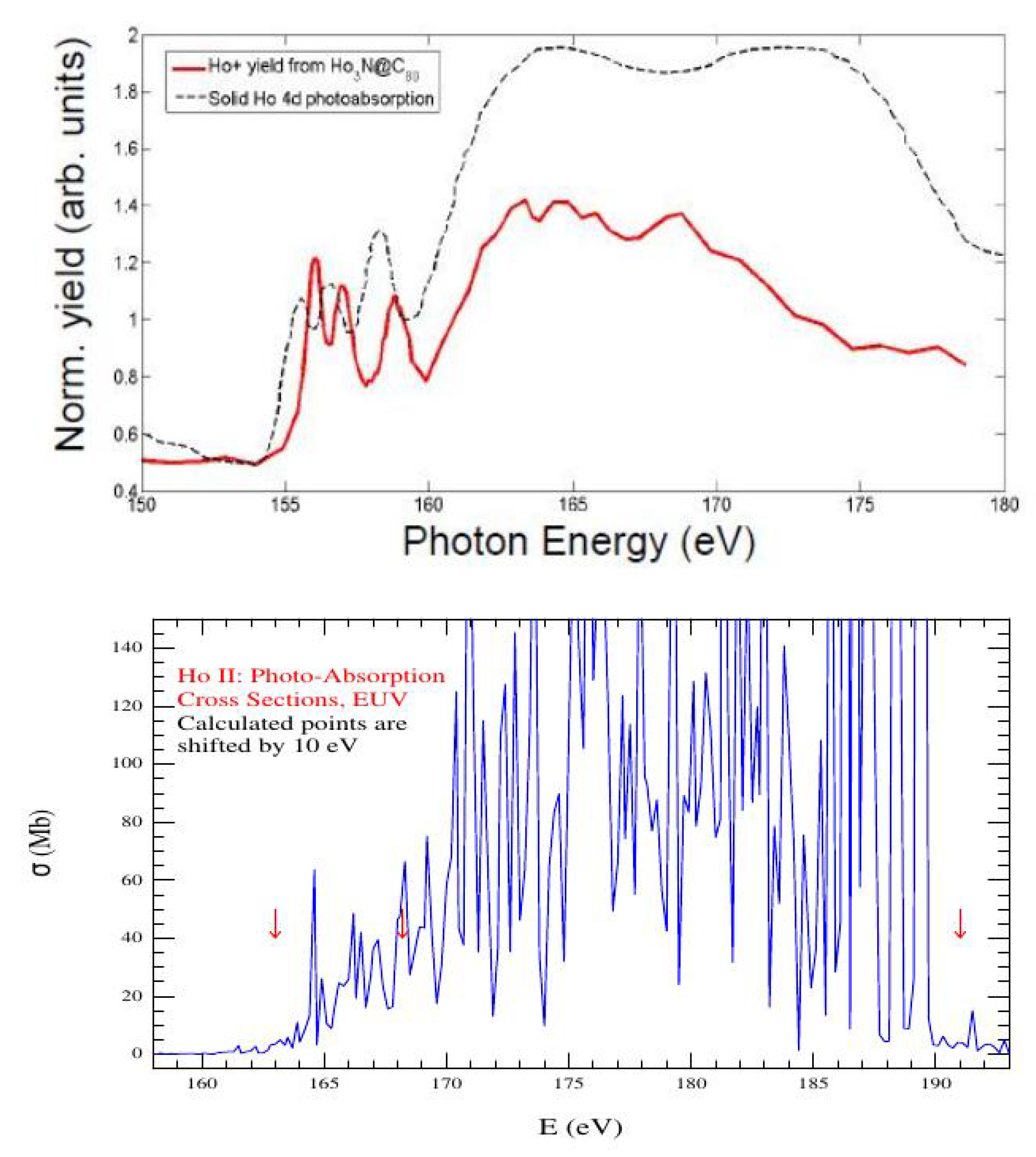
We found one experimental spectrum of a lanthanide, Ho II, measured by the group at the University of Connecticut [23], who presented the results (Figure 1, top panel) at a Division of Atomic, Molecular, and Optical Physics (DAMOP) meeting of the American Physical Society in 2016. The red curve in Figure 1 corresponds to the Ho II yield from fragmentation and the black dotted curve to solid Ho photoabsorption. The measured energy range, 150–180 eV, is in the soft X-ray region and is much smaller than that covered for Ho II in the present work. In Figure 1, the lower panel compares the present Ho II photoabsorption spectrum with the experimental one obtained by Obaid et al. [23]. The comparison indicates that the black curve is due to the photoabsorption of the spectrum of Ho II following photo-fragmentation. Although there is an energy shift of 10 eV in the predicted spectrum, we find very good agreement in the features between the two spectra. Similar to the observed feature, the predicted spectrum shows a rise in line strength that increases with the energy and remains strong over an energy range before dropping off at about 190 eV. The observed spectrum is a smooth curve since the spectral lines have been averaged out by the bandwidth of the experimental set-up.

4.2. Benchmarking of Energies

A small set of energies, with 10 levels for brevity, of each of the 25 lanthanide ions is presented in Table 3. The total number of energy levels, $N_E$, obtained from the set of configurations, and the total number of dipole allowed (E1) transitions, $N_{E1}$, obtained among them are specified at the top. $N_{E1}$ is the subset of the total number of combined allowed and forbidden transitions, $N_T$, specified in Table 1. $N_{E1}$ also corresponds to the number of transitions included in producing the photoabsorption spectrum for the ion.

Table 3 also benchmarks the present energies with the measured values, largely from Martin et al. [12], which are available in the NIST [13] table. There are two reasons for the comparison of a small set. With a larger number of levels, the comparison table will be very long with 25 ions. The other reason is the difficulty in the correct matching of levels to compare. Although only 10 energy levels have been used for the comparison with measured values for each ion, some of the ions have a relatively large number of levels available in the NIST table and some do not have any except for the ground angular momentum. A significant number of levels are not assigned full spectroscopic designation. The comparison of energies in Table 3 reveals the complex issues in the spectroscopic identification of levels. The NIST tables show the large mixing of the levels from different LS states as well as configurations, indicating possible variations in the spectroscopic designations for the level from various theoretical approaches. In most cases of the present lanthanide ions, NIST provides only partial identification for a level, the J-value, and the parity. Similar to those in NIST, SS provides the final spectroscopic identification based on the leading percentage contributions of the configurations and states. The leading percentage contribution depends on the method being used and the wavefunctions describing the atomic states. Some differences in potential or wavefunction representation in various approaches usually introduce differences in identification. However, general agreement on the spectroscopic identification can often be found among most of them. Nonetheless, these differences in identification are found to be more noticeable for lanthanides.

Identification becomes sensitive to perturbations from the mixing of levels and configurations. This is not unusual for large atomic systems with many electrons, such as lanthanides, which have highly sensitive electron–electron interactions. We attempted to match the levels with the exact identifications, such as the J-values and parity and any specified configuration, for the energy comparisons. In some cases, it appears that better agreement exists if the sequential calculated energies of the same parity are compared with the observed values, which brings the question of the possibility of higher accuracy for the calculated values than the assigned J-values, which are affected by the percentage contributions of other levels. Parity is not affected by percentage contributions.

We adopted a matching scheme for the calculated optimized set of energies to compare them with the measured energy levels. We first ensured that the calculated ground level agreed exactly with those in the NIST table, and that the other fine structure levels of the ground state matched. Next, we compared the level energies with the exact identifications for both the calculated and experimental levels. However, if there were missing L and S numbers in the NIST table or an unusual difference in the values or order of levels was noticed, we compared the levels with the same J-values and parities, and the configuration. If the NIST table did not provide L and S values, we used those designated by SS.

We found that, for higher excited levels, the calculated values tend to diverge towards larger values than those of the measured ones. During optimization, we made an attempt to reduce this divergence even when the energy order was shifted. The energy levels of the 25 ions are discussed below.

Ho I-III:

For Ho I, the comparison encountered problems due to differences in the spectroscopic identification of levels. The NIST table presents the full spectroscopic identification of the ground state ${ }^4{I}^o$ and its four fine structure levels. The present results agree with them, with about 20% uncertainty in the values. Given the difficulty encountered due to the sensitivity of electron–electron correlation, this agreement can be considered good. The NIST table does not give complete identifications for the next four sets of levels. Thus, in Table 3, we list them with the L and S values of the calculated levels from SS that have the same J and parity. In the next four levels of Ho I in Table 3, we see that the differences in energy values vary significantly. The last two levels in the table have been selected following their energy positions in the calculated energies. The comparison with the measured values is good in regard to the sensitivities of Ho I.

The problem in the proper matching of levels is also one of the reasons for the mismatched order of the calculated energy levels with those of the measured levels. To match for comparison, we have used largely the NIST energy order and SS identifications for the designation of levels. However, even with such identifications, the comparison shows poor to good agreement. Hence, the energies of Ho I may require a larger configuration set for better optimization in future work.

The calculated energies and order of the low-lying Ho II levels have good agreement with those in the NIST [13] table. However, NIST does not provide spectroscopic values of the total spin S and orbital angular momentum L. Hence, the identifications produced by SS are used to designate these values in the comparison table.

The calculated energies of Ho III are comparable but are lower than those of [12]. The calculated energy order also differs after the first five levels and thus introduces a discrepancy. Further optimization in the wavefunction expansions increased the difference between the calculated and measured values. Hence, the present set of values is chosen for overall agreement. It is possible that the differences in energies between the calculated and measured values are due to uncertainties introduced by configuration mixing and hence the lack of proper spectroscopic identifications of levels.

Er I-IV:

The energy levels of Er I show, in general, good to poor agreement with the measured values. These ions were challenging computationally and in terms of spectroscopic identification in similar ways to the Ho ions. The sensitivity of the electron–electron interaction caused the repetition of the computation many times to optimize the wavefunctions to match the ground and excited levels. When the energy levels are similar to those of the observed values, the identifications and order of levels would be different from those of NIST. We adopted the comparison strategy mentioned in the above section for the best matching of the levels and the comparison of energies, which showed good to fair agreement.

The calculated energies of Er II show agreement similar to that for Er I. Except for one odd parity state, ${ }^4{I}^o$, none of the Er II levels, including the ground state, have full spectroscopic designation in the NIST table. NIST provides J-values and parities. Hence, the levels have been assigned with the L and S values given by SS. For the Er II comparison, with the preservation of the parities and J-values, we find that the ${ }^4{I}^o$ levels show the largest discrepancy. This discrepancy would have been smaller if we had considered configuration $4f^{11}5d6s$ instead of the NIST-assigned configuration $4f^{11}6s^2$. The agreement is quite good with the $4f^{11}5d6s$ odd parity level of J = 13/2. Hence, the comparison will need verification with other accurate calculations or experiments.

The optimization produced calculated energies for Er III that were somewhat lower than the measured values, but they remained in fair to good agreement. The NIST table assigns spectroscopic designation only for three levels. Hence, while the parity and J-values are matched for comparison, the L and S values are assigned following those from SS.

The calculated energies of Er IV can be discussed in terms of the same points as for Er I-III. For Er IV, the calculated values are somewhat higher than the values quoted in NIST. The agreement is fair to good.

Tm I-V:

Table 3 shows good to poor agreement between the calculated and measured energies of Tm I–Tm-V. The reasons for the differences are the same as those for the Ho and Er ions. These lanthanide ions have strong electron–electron interactions that can be perturbed easily by slight changes in wavefunction, similarly to other lanthanides. The problem of the matching identification of levels and partial identification introduced uncertainty in the comparison of the levels and hence caused a discrepancy between the calculated and measured energies.

The Tm I energies are very sensitive to the configurations and Thomas–Fermi scaling parameters. A slight change in the scaling parameters, which expands or contracts the wavefunction, would affect the order and values of the levels and the energy values. It is also difficult to compare them as NIST gives the configurations but is missing the L and S values. The energies from SS are closer to the energies of the NIST values if the quantum states designated to them are ignored. This again highlights the need for high-accuracy calculations and experimental measurements.

Tm II and Tm III show similar identification problems. NIST provides a number for the total angular momentum, instead of an alphabetic character, and no spin information. Thus, the present comparison is made largely based on the order of matching of the parity and J-values. For Tm II, levels 6 and 7 appear to have reverse identification. The agreement between the present and the compiled set of NIST is good to fair. The comparison of Tm III can be considered good on average.

For Tm IV, the present values in general are in good agreement with the measured energy values of Martin et al. [12]. However, two levels, ${ }^{3}H$ and ${ }^{3}F$, both with j = 4, appear to be misidentified, with a change in energy values of 0.114 Ry and 0.0514 Ry. The identification of these levels can be adopted easily in the reverse order as their leading percentages are very close, 60 and 63, respectively. The NIST table list only seven levels. Hence, the three additional levels in Table 3 are calculated ones.

For Tm V, there is no energy level available except for the ground level $4f^{11}{(}^3{I}_{15/2}^o)$, which we confirm in the present work.

Yb I-VI:

Yb I identification for the four levels above $4f^{14}6s6p{(}^3{P}^o)$ is not defined in the NIST table and hence the SS identifications that match the parity and j-values are used. Yb I also perturbs easily with a slight change in the spatial extension of the orbital wavefunctions. They were optimized to match the observed low-lying energies by Martin et al. [12], but the order of the spectroscopic identifications has less agreement. The present comparison shows large differences, but they can be reduced by the matching of the configurations, which was not considered.

Yb II also had very a sensitive electron–electron interaction potential, which would change the order of the energy levels or the energy values with a slight change in the wavefunction. Since the NIST table reports an over 90% leading percentage for the lowest-lying level designations, the present optimization focused more on the energy order than the energy values to achieve it. The comparison shows fair to good agreement between the calculated and observed values.

The calculated energies for Yb III are seen to be in good agreement with the measured values. SS identifications were used for the levels whenever NIST did not have them.

The calculated Yb IV energies agree well with the measured values. The identifications of levels given in Table 3 correspond to those predicted by SS as most levels are not identified in the NIST table.

There is no measured energy for Yb V available on the NIST website, except for the ground level designation of ${ }^3{H}_6$. Our calculated ground level agrees with the level designation. Hence, all energy levels of Yb V in Table 3 are calculated values.

Yb VI has 68 levels belonging to the ground configuration $4f^{12}5p^5$. This means that there is no low-lying allowed transition. The transition energy for the first dipole allowed transition of the ground level ${ }^4{I}_{15/2}^o$ is at about 1 Ry. The NIST table does not contain any observed energy of Yb VI besides giving the J-value of the ground level, which was predicted by [14]. The present ground level agrees with this J-value. We noted that a different set of configurations can also produce energies for Yb VI that are different in values and energy order from the present set. It also gives a different spectroscopic designation for the ground level. We choose the present set as it has the same ground level configuration as that given in the NIST table. There is a need for observed values as guidance to determine the configuration set for the ion.

Lu I-VII:

The optimization of wavefunctions for the ordering of the Lu I energies was found to be sensitive to the presence of excited configuration $5d^{2}6s$, whose levels would raise the ground level to a higher excited state. A ground level that has even parity needs odd parity levels for dipole allowed transitions. Hence, we attempted to perform the optimization of the energies of odd parity levels such that lower energies were achieved for the levels through the optimization of the wavefunctions. The resultant set of energies, as seen in Table 3, shows good to poor agreement with the set of NIST.

The energies of Lu II show good agreement with the measured values.

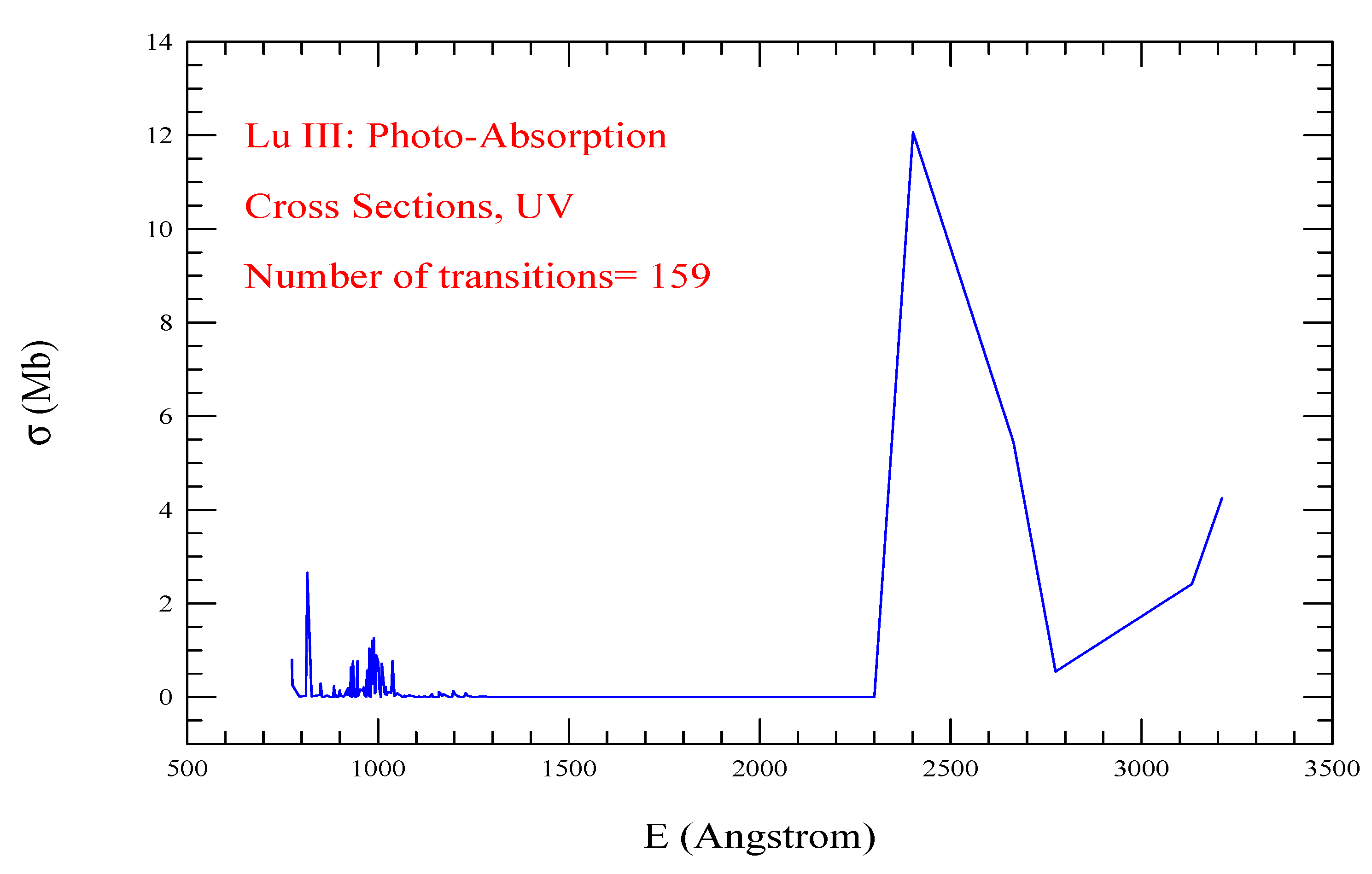
For Lu III, we are able compare only a limited number of energy levels since most of the energies in the NIST table belong to orbitals that are not accessible to SS. However, the comparison shows good agreement. The NIST table does not list the energies of configuration $4f^{13}5d^2$, which is included in the present calculations and found to produce a large number of bound levels. Being a ${ }^2{S}_{1/2}$ level of configuration $4f^{14}6s$, the ground level can have dipole allowed transitions only to ${ }^2{P}_{1/2,3/2}^o$ and hence only a limited number of transitions is possible. We obtained only 159 dipole allowed transitions, including those to levels of ${ }^2{S}_{1/2}$, of the ground level to be included in producing the spectrum. We included a few other configurations that generated bound levels but have not been observed.

For Lu IV, overall good agreement is found between the calculated and measured values. The levels have been identified following SS, as NIST does not provide the full spectroscopic designation of any excited level.

For Lu V, the calculated values of the ground level and lower energies agree well with the measured values listed by NIST [13]. The full spectroscopic designation of any excited level of Lu V is not available in the NIST table. The leading percentage values in the NIST table indicate highly mixed states. Hence, in Table 3, these levels have been designated with the $LS$ term obtained from SS when the J-value and parity match for both the calculated and observed levels.

For Lu VI, there is no fine structure level, except for the ground level, available in the NIST table. We carried out the optimization of the levels such that the absolute values were the lowest and the ground level matched $4f^{12}5p^6{(}^3{H}_6)$ given by NIST. All nine excited levels of Lu VI in Table 3 are calculated values.

There are no fine structure energy levels for Lu VII in the NIST table, except for the ground configuration $4f^{13}5p^4$, with which the present work agrees. Similar to Lu VI, the optimization of energies was carried out by lowering the energy values.

4.3. Benchmarking of Transitions in Lanthanide Ions

We perform a comparison of a number of A-values of the present lanthanide ions in Table 5 with the compiled values available at NIST [13]. A limited number of A-values for some ions of Ho, Er, Tm, Yb, and Lu is available in the NIST [13] compilation table. The NIST references for the A-values of lanthanides are Meggers et al. [15], Morton [16], Komarovski [17], Wickliffe and Lawler [18], Sugar et al. [19], Penkin and Komarovski [20], and Fedchak et al. [21]. The comparisons show variable agreement between theory and computation. The order of magnitude agrees, and the absolute values agree to different degrees. Typically, the A-values calculated from two different approaches or programs show general agreement in the transitions, but not for all transitions. Hence, in the present case, the overall agreement should be good given the sensitivity of electron–electron interactions and the impact of slight changes in the wavefunction in lanthanides.

We compare only a couple of transitions. The reason for this is that the comparisons are expected to have a certain amount of uncertainty due to the lack of proper spectroscopic identification, particularly of the excited level to which the ion is excited. This problem is due to the high mixing of levels. The other issue is the identical set of quantum numbers. A large number of possible angular momenta resulting from the vector addition of the individual angular momenta of a large number of electrons introduce multiple sets of similar quantum numbers that can be assigned to a level. A single configuration can produce a number of levels with different energies but with the same J-values and transitions that occur between the same set of two J-values of the transitional levels belonging to the same set of configurations, although with different energies. The small differences in energies, such as for lanthanides, do not resolve these issues since the calculated energies are not as precise as the measured values.

The present work aims at the overall improvement of the accuracy for collective features of transitions, such as those observed in lanthanide ions.

4.4. Spectral Features of Lanthanide Ions

Ho I–Ho III:

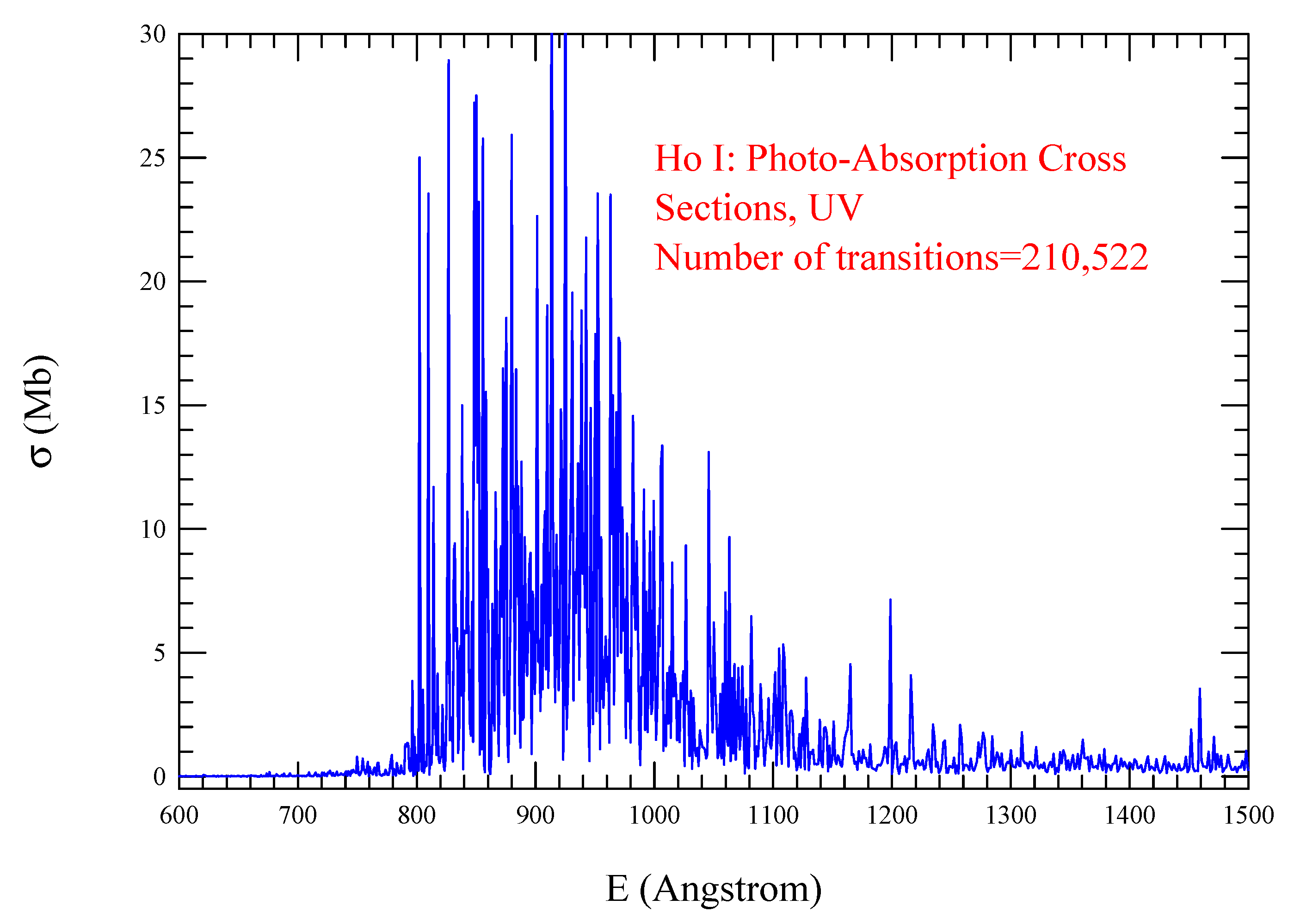
The photoabsorption spectrum of Ho I is presented in Figure 2. A total of 210,522 transitions were included to plot the spectrum. However, those with very low cross-sections were beyond the scale of the plot. Figure 2 shows that the dominant strength of lines lies in the UV range of about 800 to 1200 Å. The range could deviate by some Å due to the differences between the calculated and measured energies.

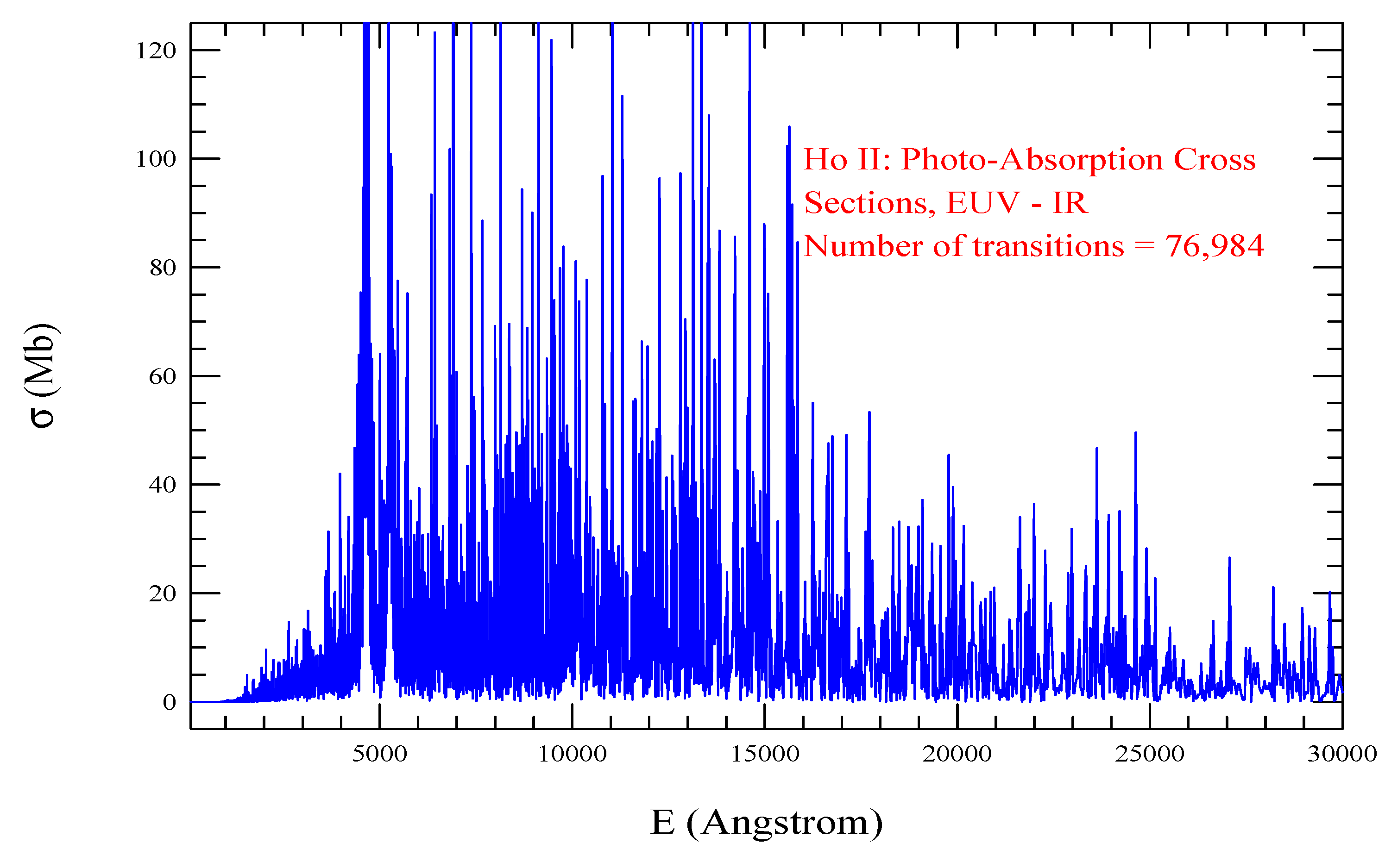
Figure 3 presents the photoabsorption spectrum of Ho II, which includes 76,984 transitions. However, very weak transitions lay outside the range of the plot. The figure shows the visible presence of lines from 4000 Å in UV to 18,000 Å in the IR region.

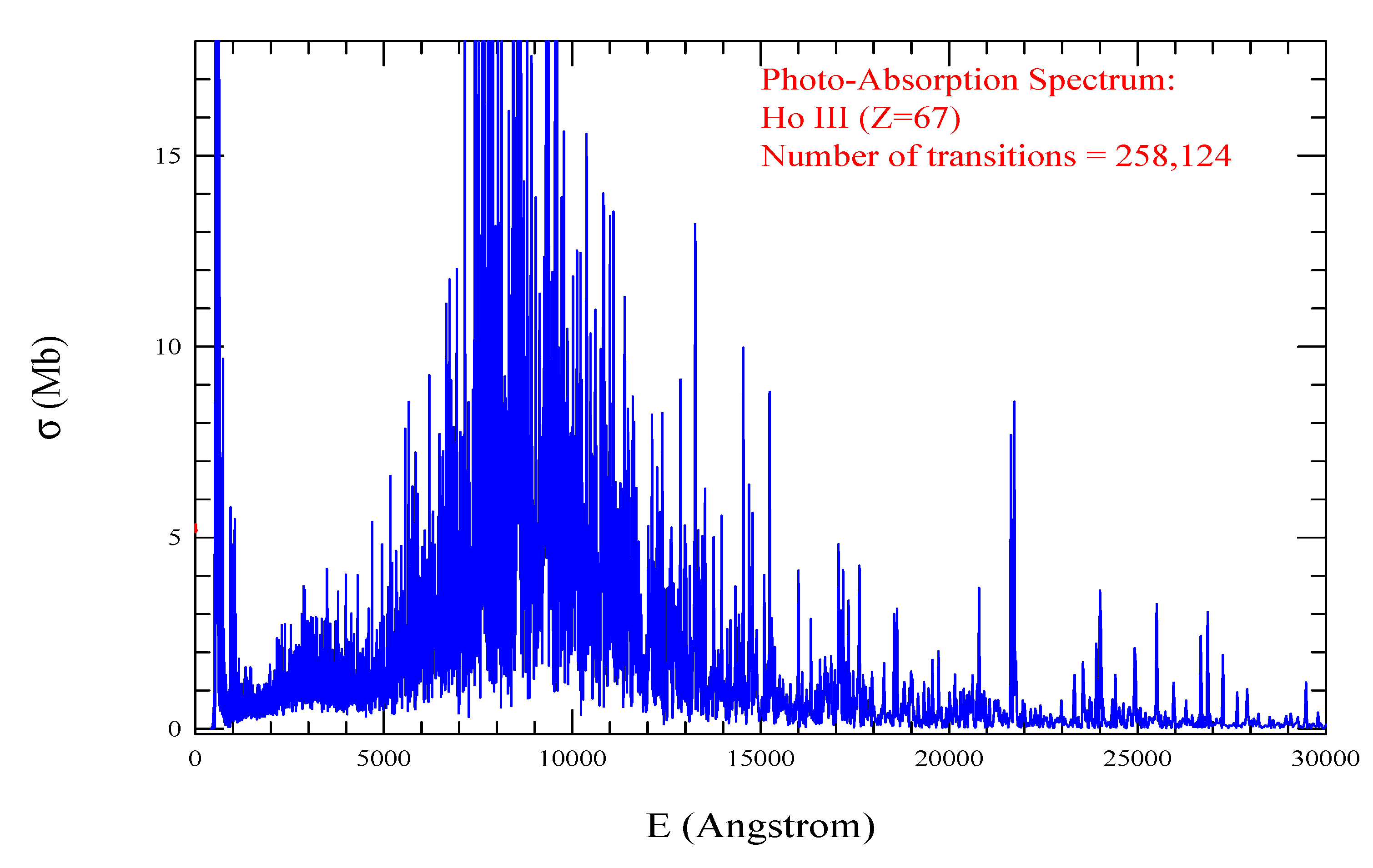
Figure 4 presents the photoabsorption spectrum of Ho III, which shows the dominance of lines from X-ray to FIR 22,000 Å. A large absorption bump is found in the wavelength range of 4000 to 15,500 Å. The number of transitions included in the figure is 258,124.

Er I–Er IV:

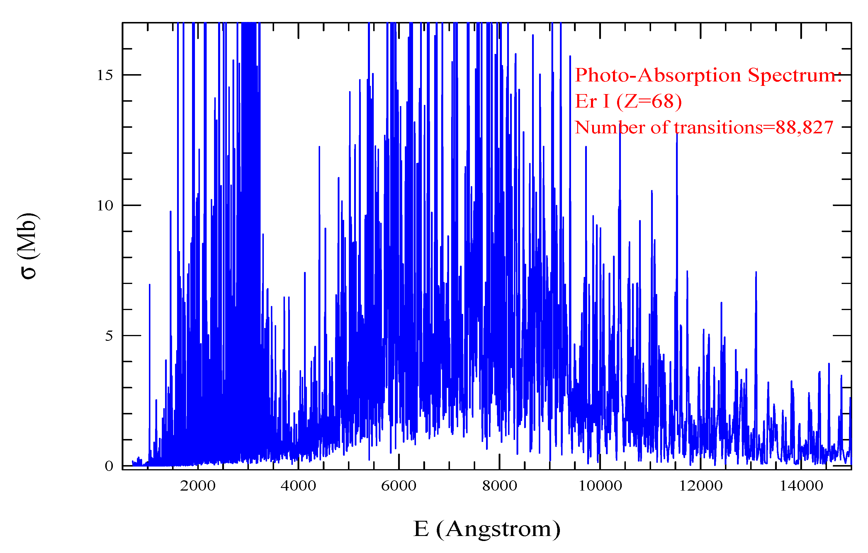
The spectrum of Er I presented in Figure 5 shows two broad features of strong lines, one in the UV region of 1000–3500 Å and the other in the O–IR region of wavelengths 4500–15,000 Å. The number of E1 transitions included in the spectrum is 88,827.

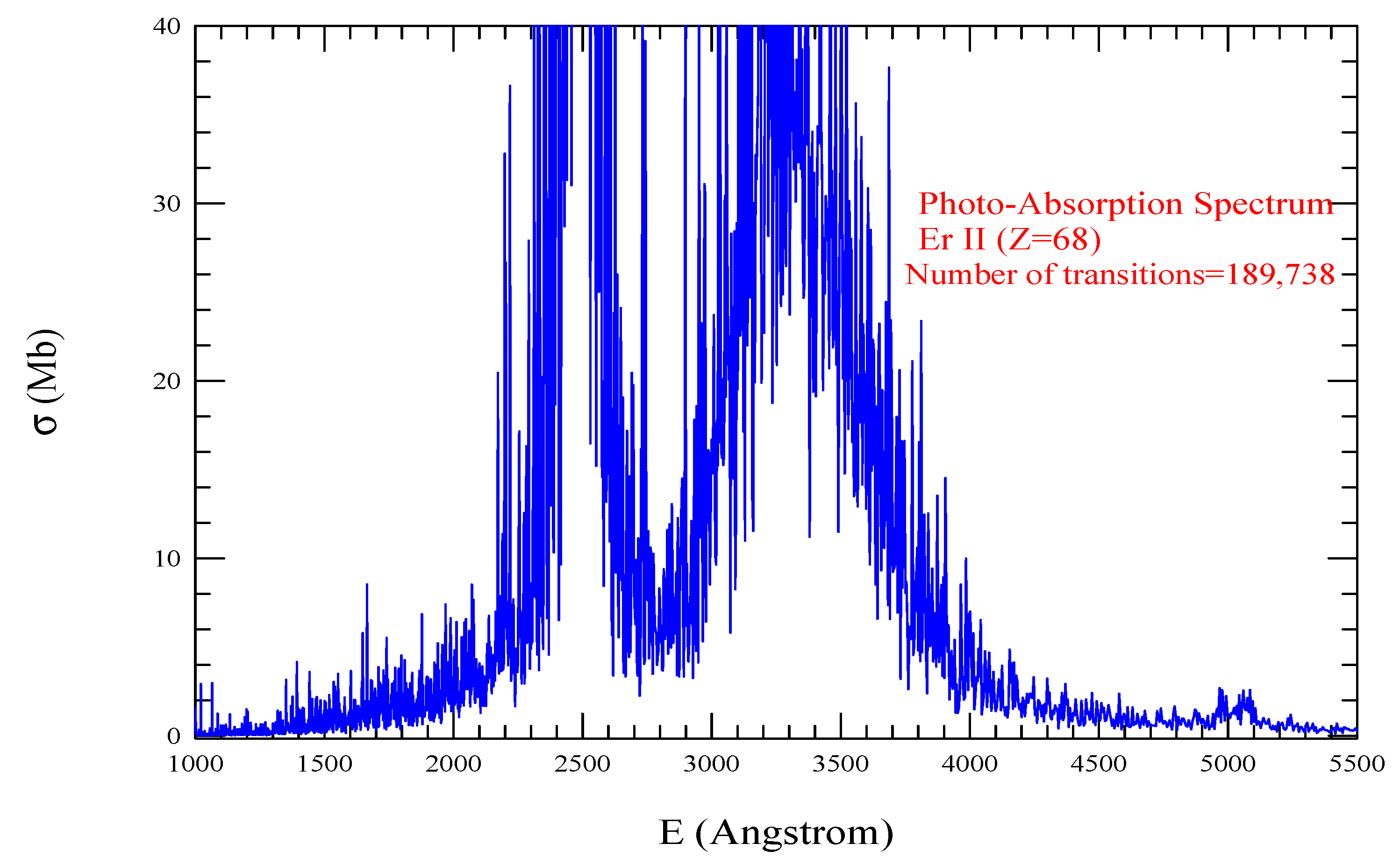
The spectrum of Er II presented in Figure 6 shows two broad features of strong lines, both in the UV region: one in the wavelength range of 2200–2700 Å and the other one in 2800–4000 Å. The number of E1 transitions included in the spectrum is 189,738.

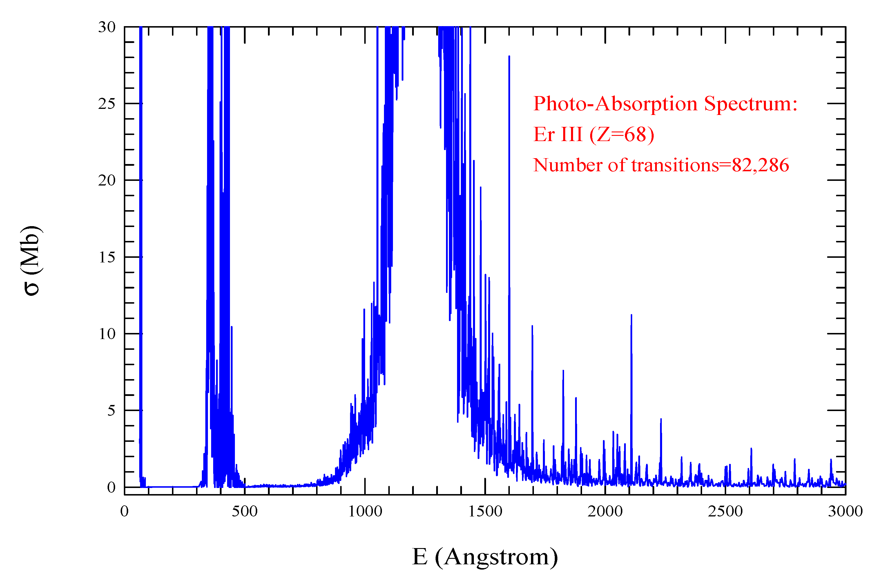
The spectrum of Er III presented in Figure 7 shows two broad features of strong lines, both in the EUV region: one in the wavelength range of 300–500 Å and the next one in 900–1700 Å. The number of E1 transitions included in the spectrum is 82,286.

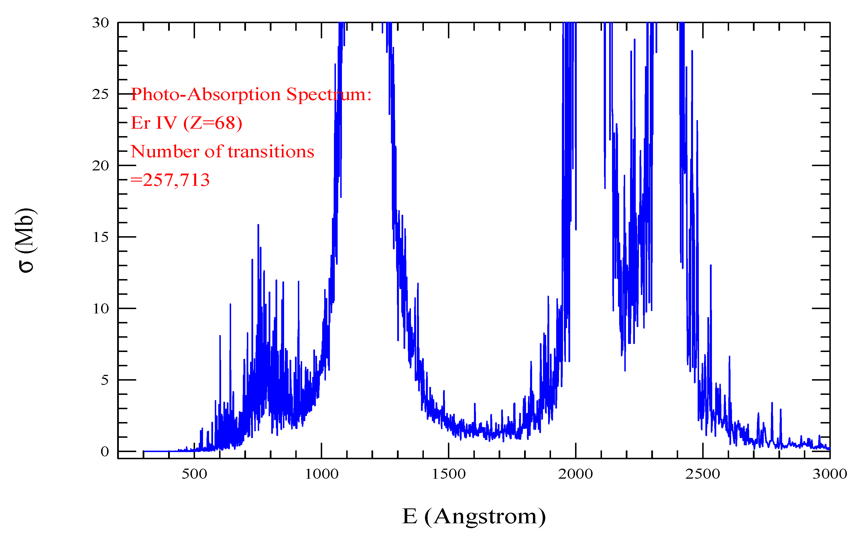
The spectrum of Er IV presented in Figure 8 shows multiple broad features of strong lines in various wavelength ranges in the EUV–UV region. The number of E1 transitions included in the spectrum is 247,713.

Tm I–Tm V:

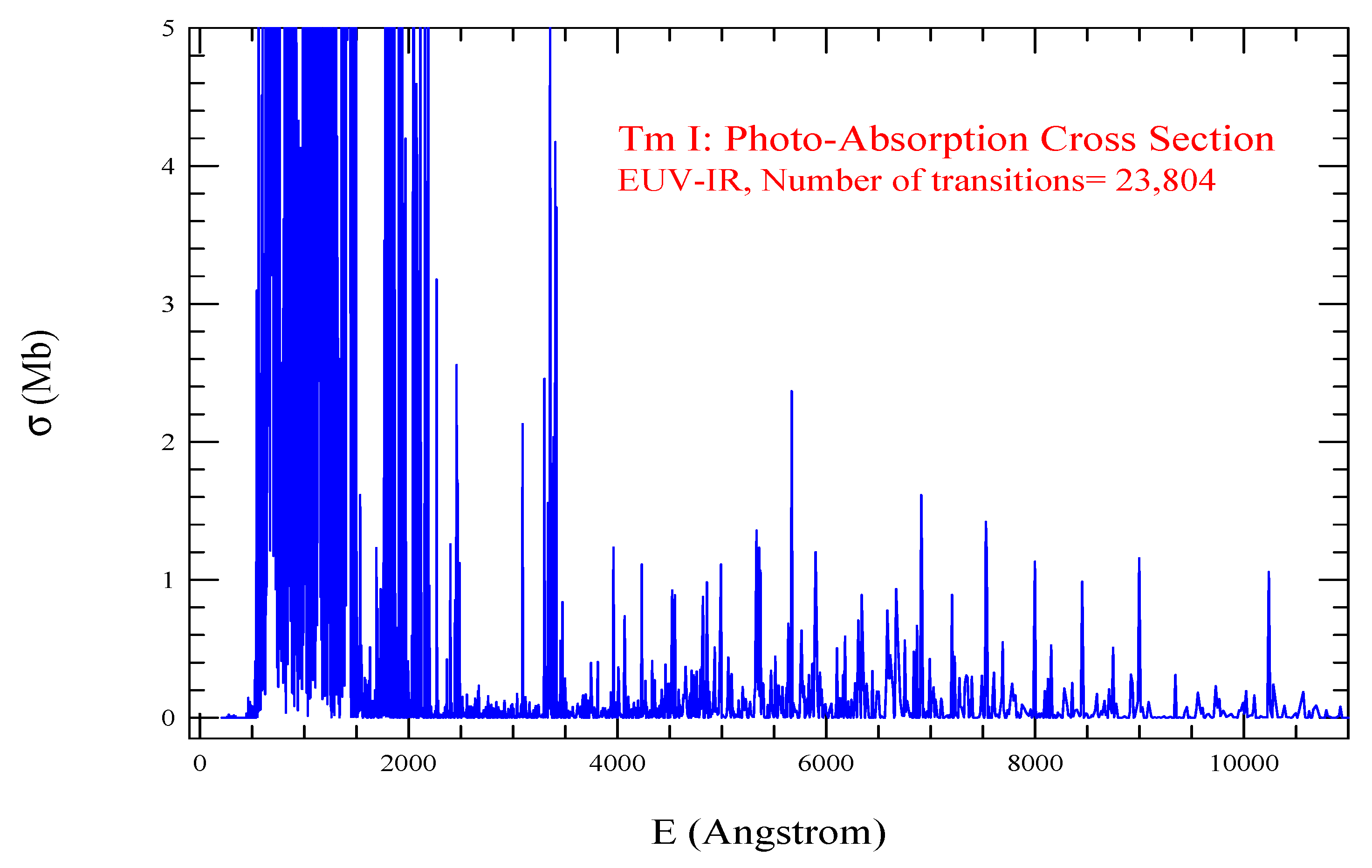
The spectrum of Tm I, presented in Figure 9, shows a few regions of strong lines; the broadest region is in the EUV wavelength range of 500–1500 Åand the next one is at about 1700–2500 Å. Beyond this, at about 3400 Å, a narrow region of strong spectral lines is noticeable. The number of transitions included is 23,804.

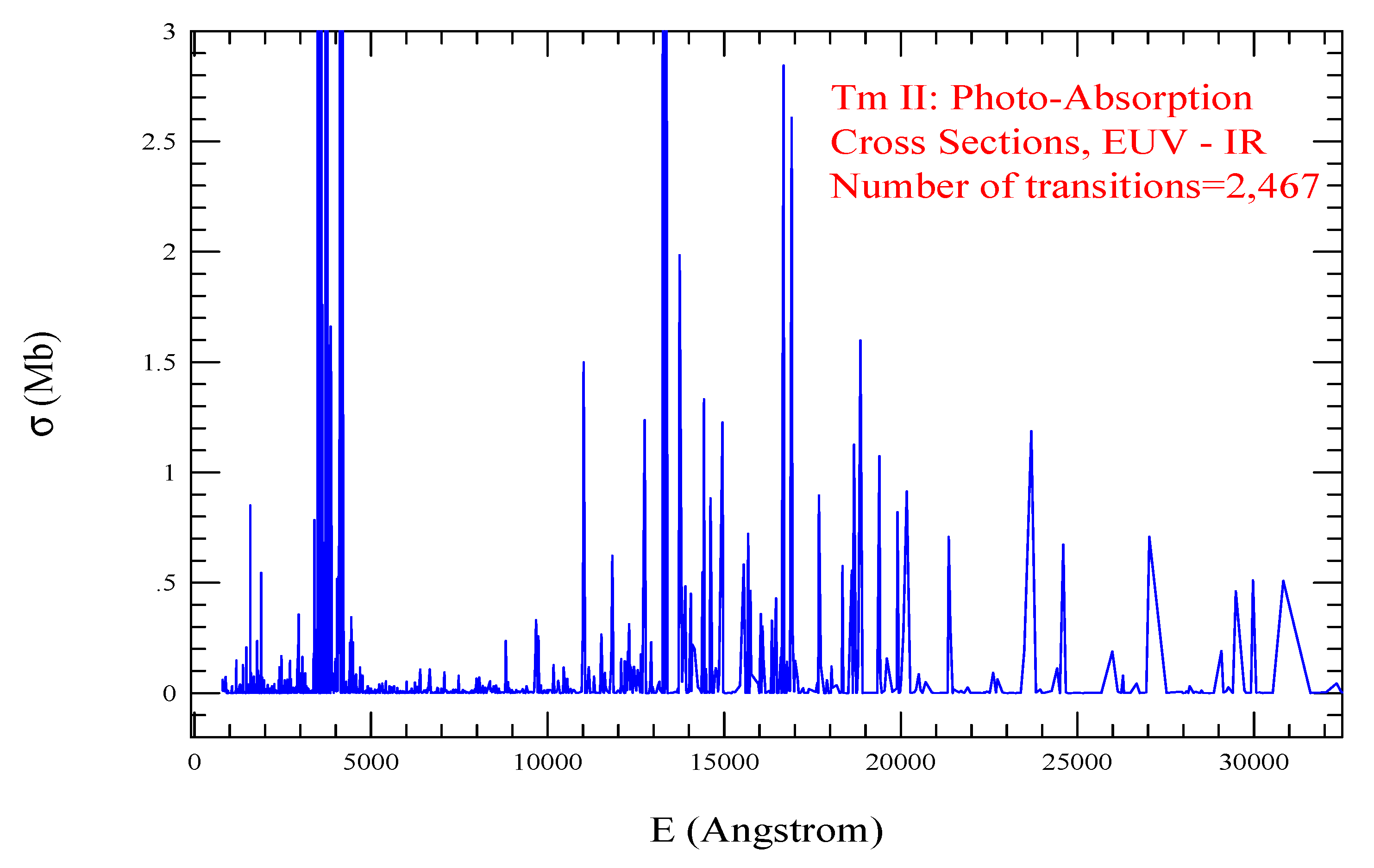
The spectrum of Tm II, presented in Figure 10, shows the visible presence of strong lines in the UV and IR regions, and almost no strong lines in the optical (4000–7000 Å) region. Compared to other lanthanides discussed here, this ion has a smaller number of transitions and a relatively wider broad feature exists in the IR region.

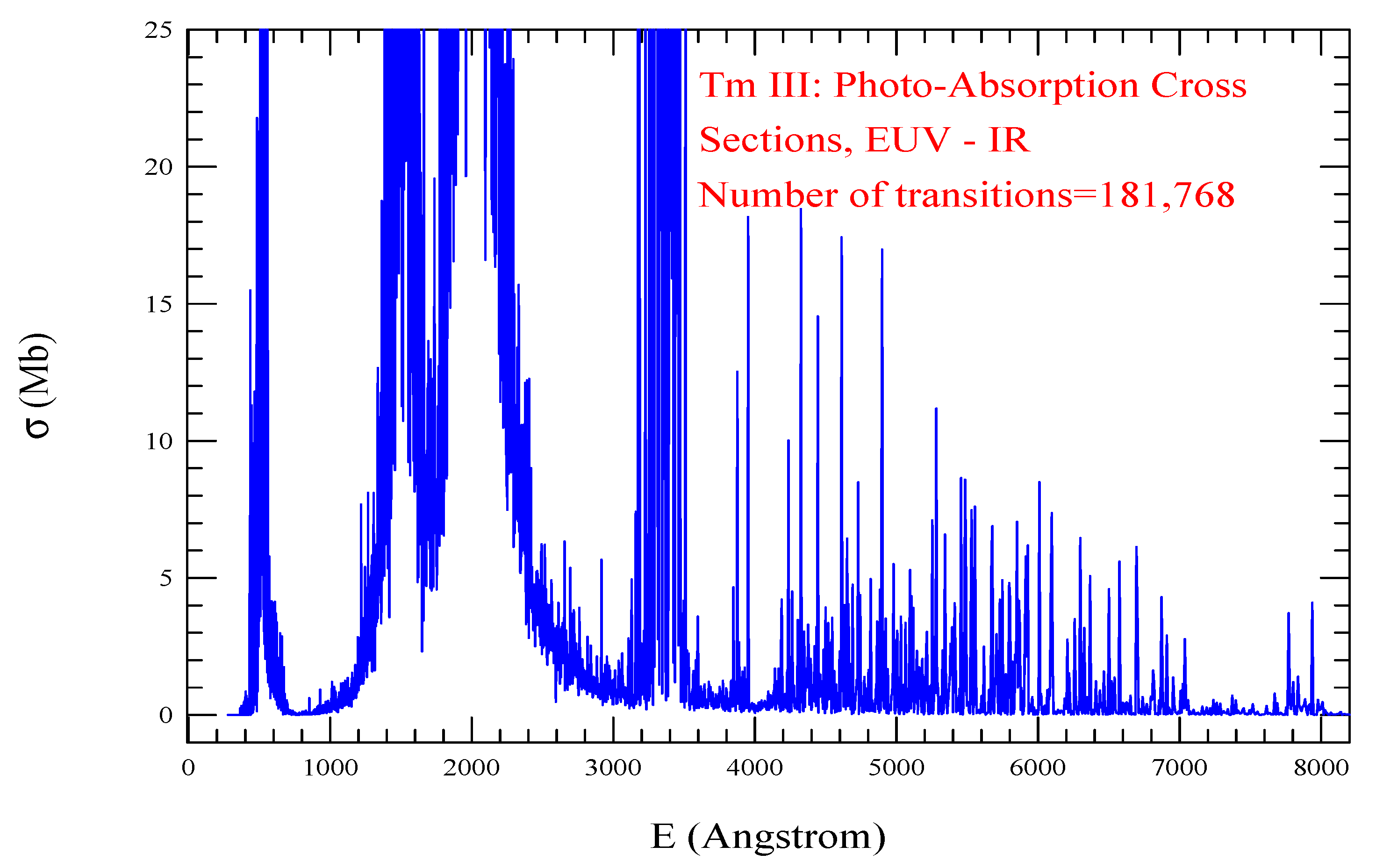
The spectrum of Tm III, presented in Figure 11, shows multiple broad regions with strong lines, from the EUV to the optical wavelength range. The widest one is in the range of 1200–2500 Å. The number of transitions included is 181,768.

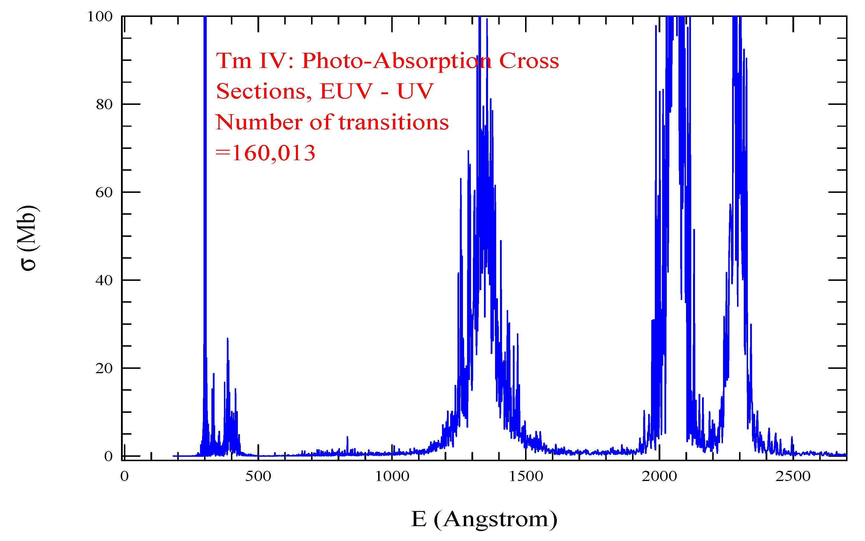
The spectrum of Tm IV, presented in Figure 12, shows four distinct broad regions, with strong lines, in the wavelength regions of EUV up to UV. The number of transitions included is 160,013.

The photoabsorption spectrum of Tm V, presented in Figure 13, demonstrates the dominance of strong lines in the energy range of EUV to UV with a gap of about 700–1300 Å. It shows multiple broad structures from the EUV to the UV wavelength range, with the widest one being in the range of 1400–1900, Å with a dip at around 1650 Å. The number of transitions included is 259,539.

Yb I–Yb VI:

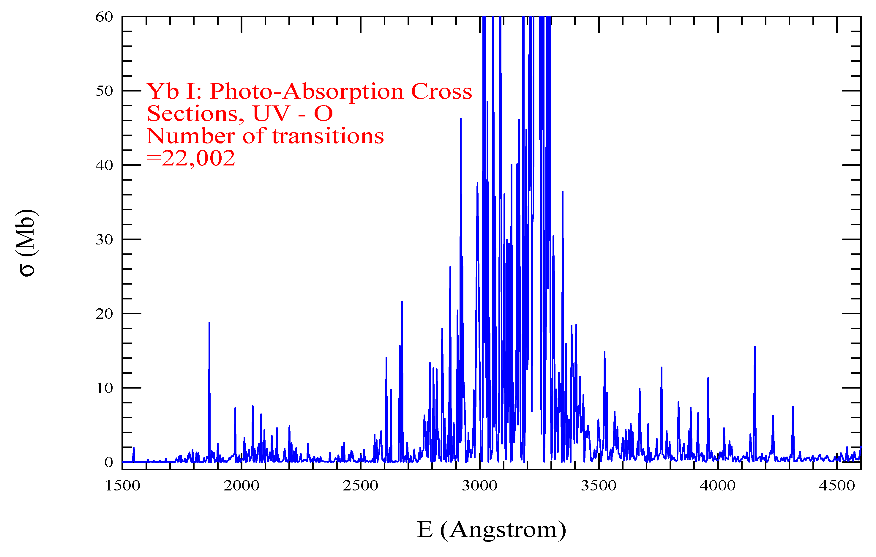
The photoabsorption spectrum of Yb I, presented in Figure 14, demonstrates the dominance of strong lines in the energy range of EUV to UV, with a broad feature in the wavelength range of about 2600–3500 Å. The number of transitions included is 22,002.

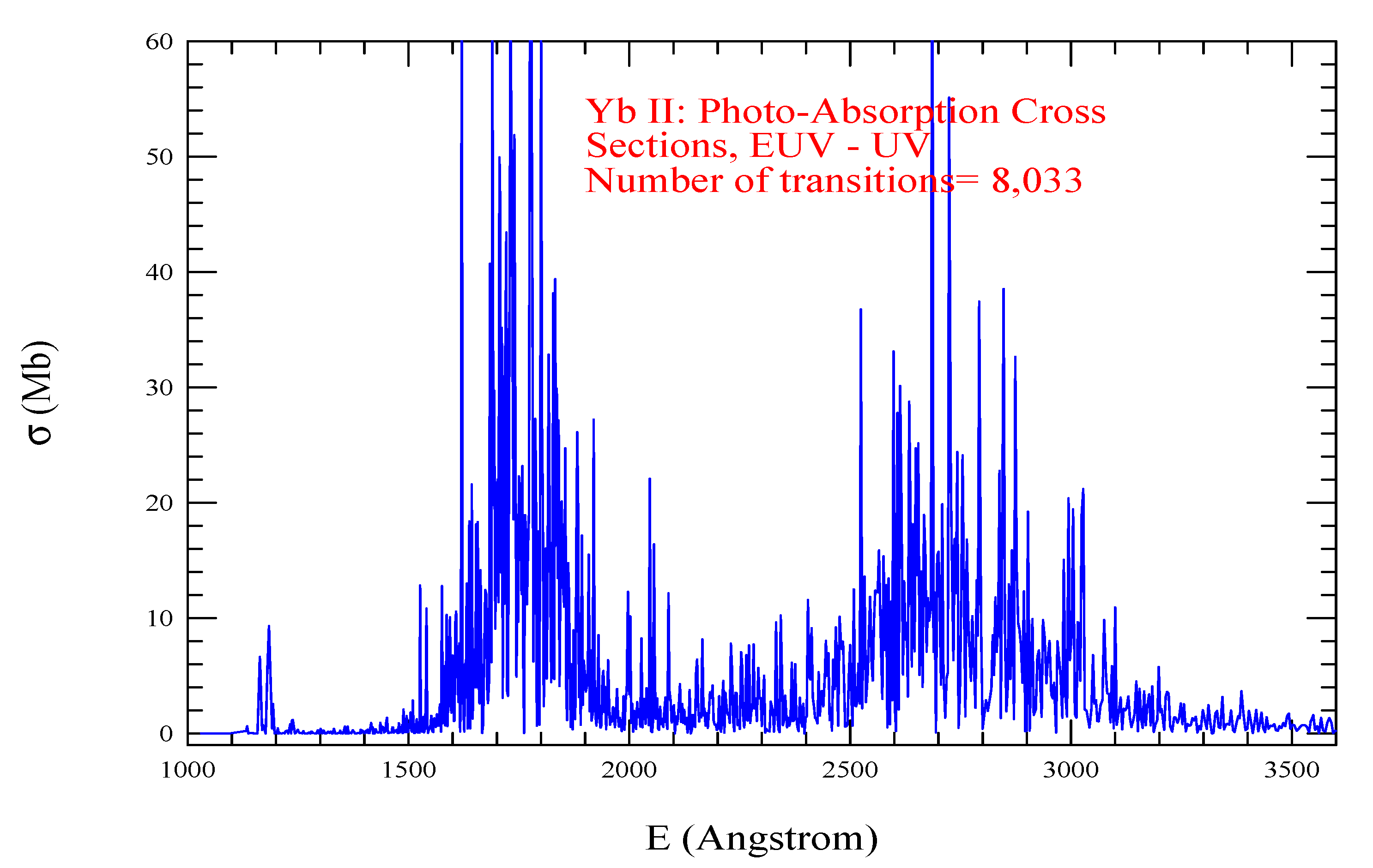
The photoabsorption cross-sections ($\sigma$) of Yb II, presented in Figure 15, show dominating strong lines in the energy region of EUV–UV. The spectrum also shows two broad features, one in the wavelength range of 1500–2100 Å and another one at 2500–3100 Å. The number of transitions included is 8083.

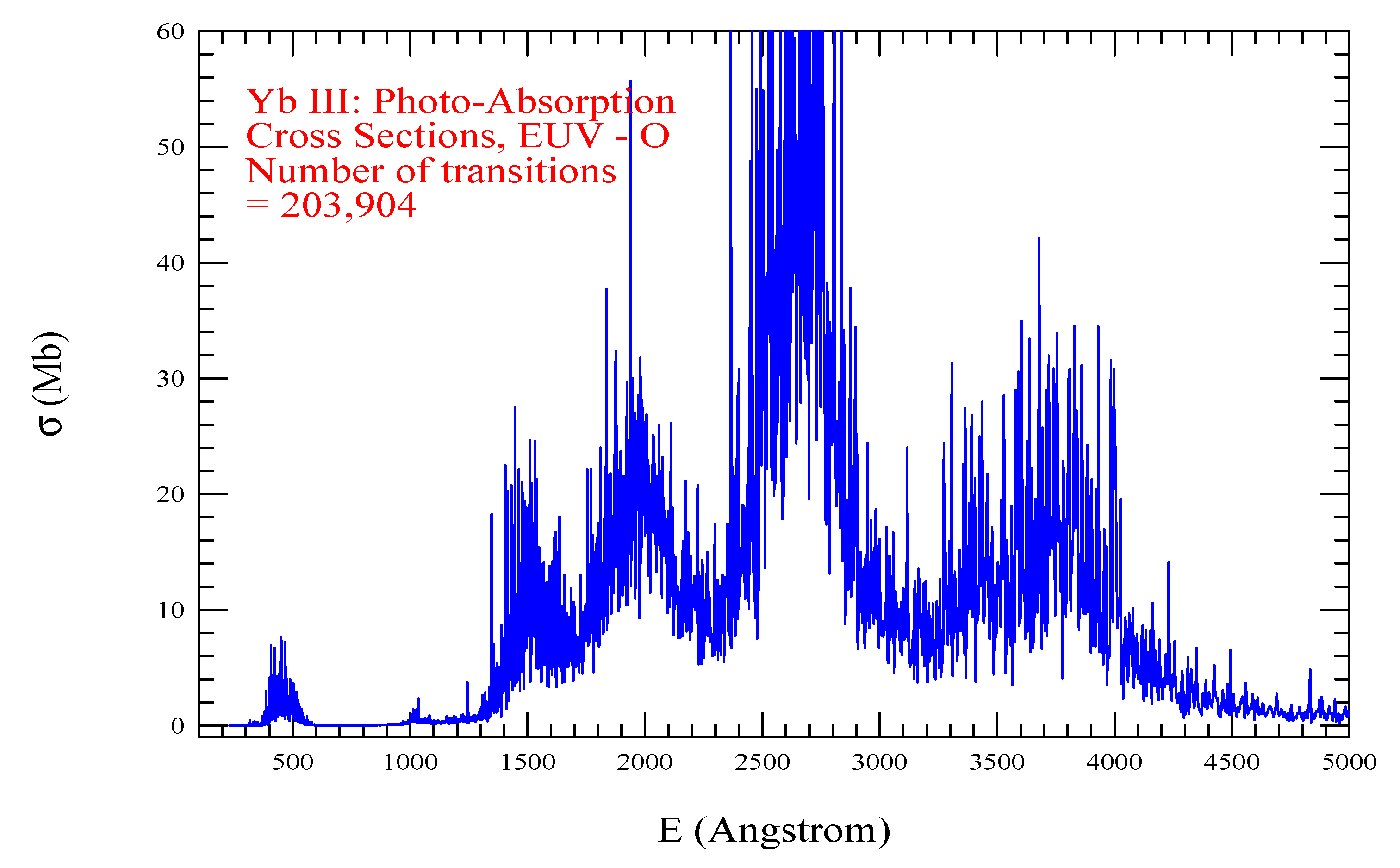
The photoabsorption cross-sections ($\sigma$) of Yb III, presented in Figure 16, has multiple broad features dominated by strong lines in the energy range of EUV–O. The strongest absorption bump is in the wavelength range of 2200–3000 Å. The number of transitions included is 203,904.

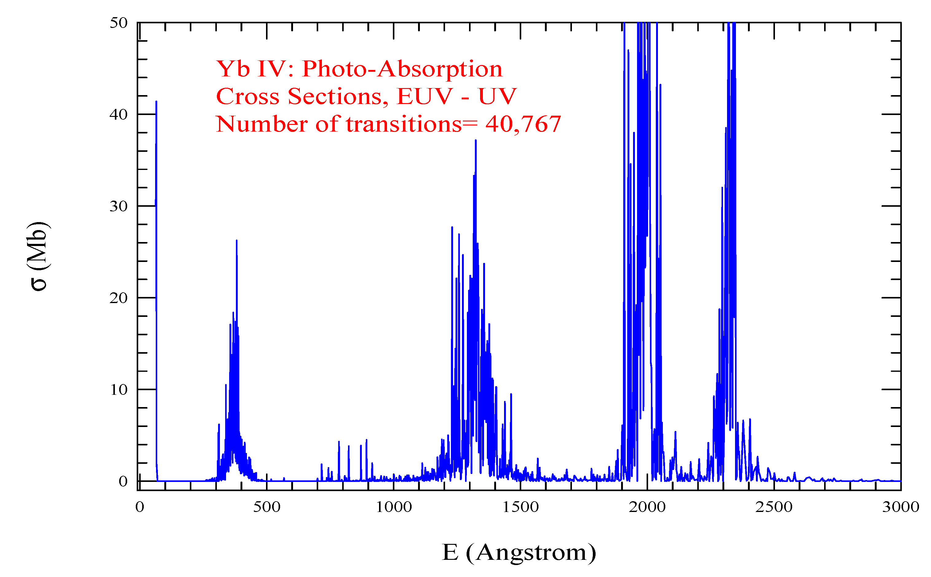
The photoabsorption cross-sections ($\sigma$) of Yb IV, presented in Figure 17, have multiple broad features dominated by strong lines in the energy range of EUV–UV. The number of transitions included is 40,767.

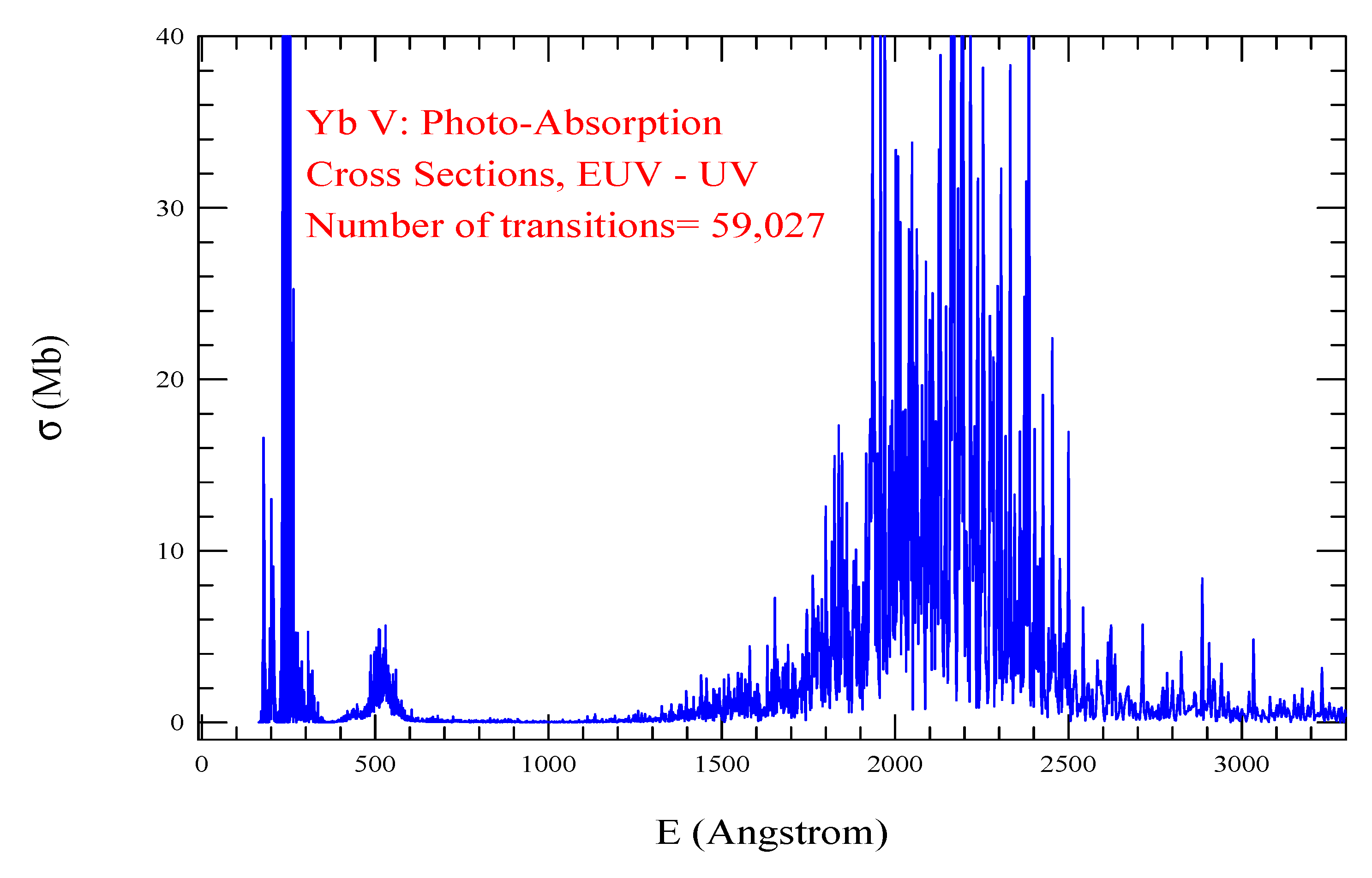
The photoabsorption cross-sections ($\sigma$) of Yb V, presented in Figure 18, show noticeable features in the energy range of EUV–UV. It has two broad features dominated by strong lines: one in the EUV region, followed by a structure of low peaks and a broader absorption bump in the wavelength region of 1600–2500 Å. The number of transitions included is 59,027.

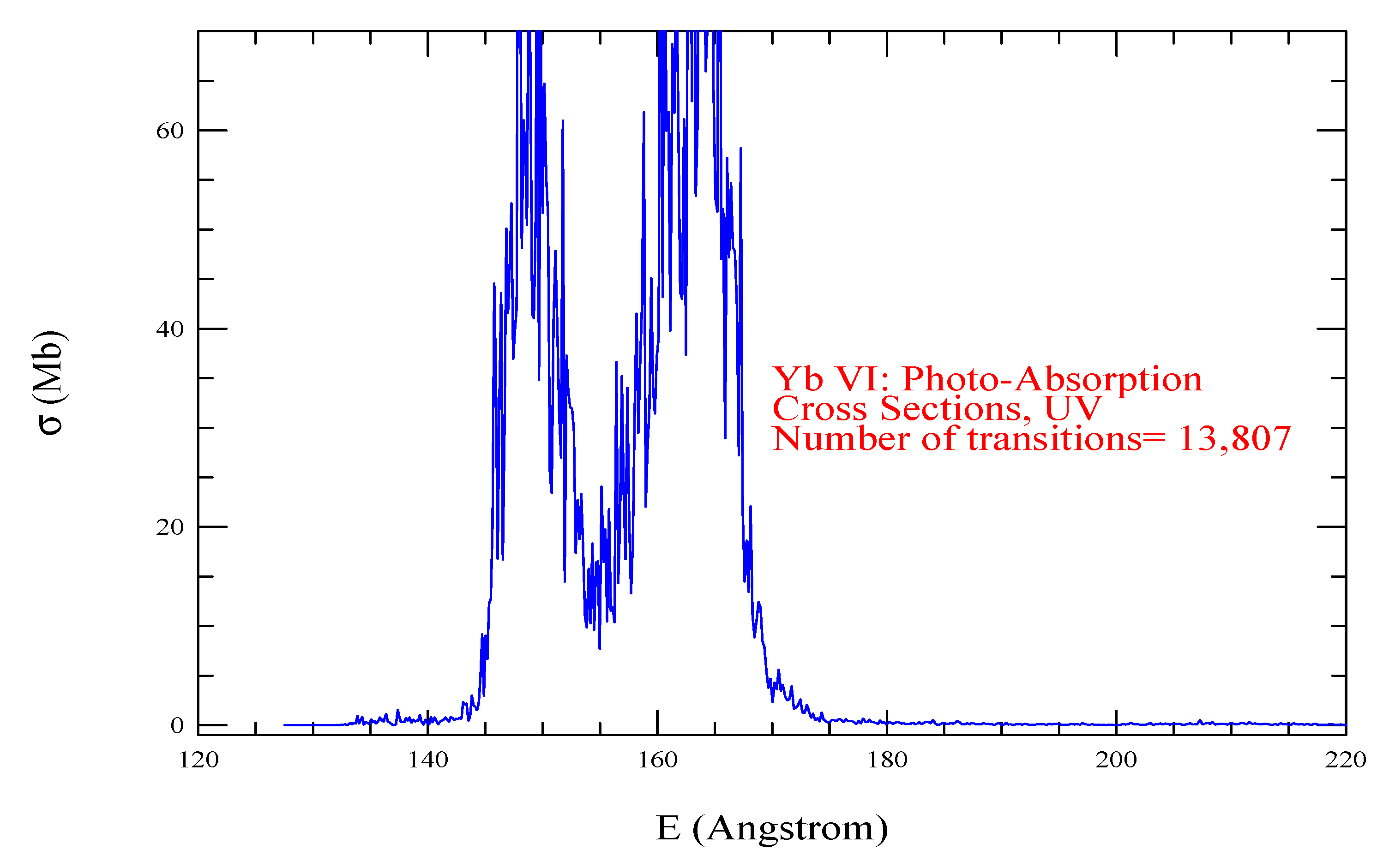
The photoabsorption spectrum ($\sigma$) of Yb VI, presented in Figure 19, shows visible features in the EUV region, particularly two absorption bumps next to each other in the energy range of 145–170 Å. The number of transitions included is 13,807.

Lu I–Lu VIII:

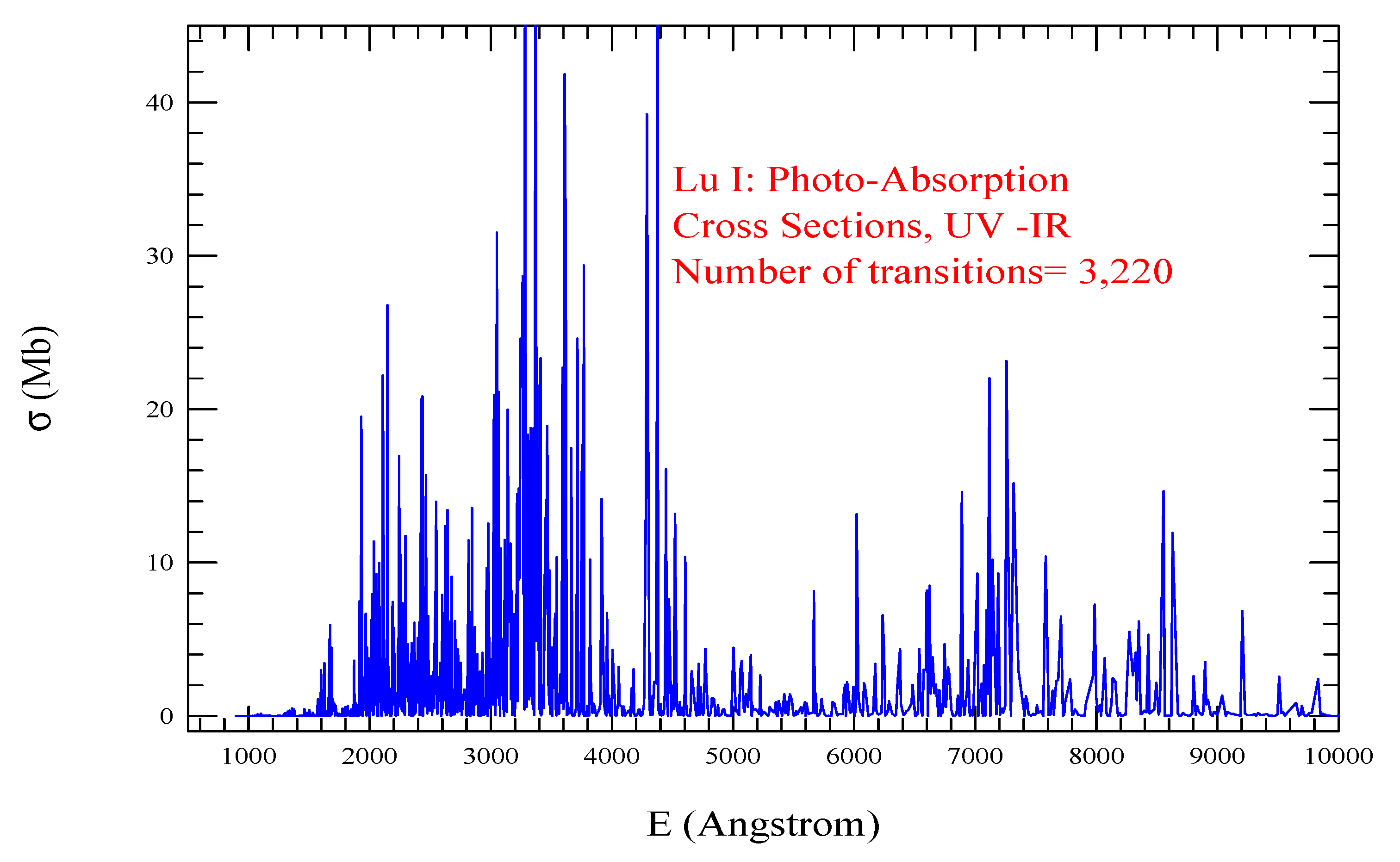
The photoabsorption spectrum ($\sigma$) of Lu I, presented in Figure 20, shows prominent strong lines in the energy region of UV to IR. It has a few broader regions of strong photoabsorption lines in the energy regions of 1800 to 3000 Å, 3000–4000 Å, and 4300–4600 Å. The higher-energy region also demonstrates the presence of some strong lines. The number of transitions included is 3220.

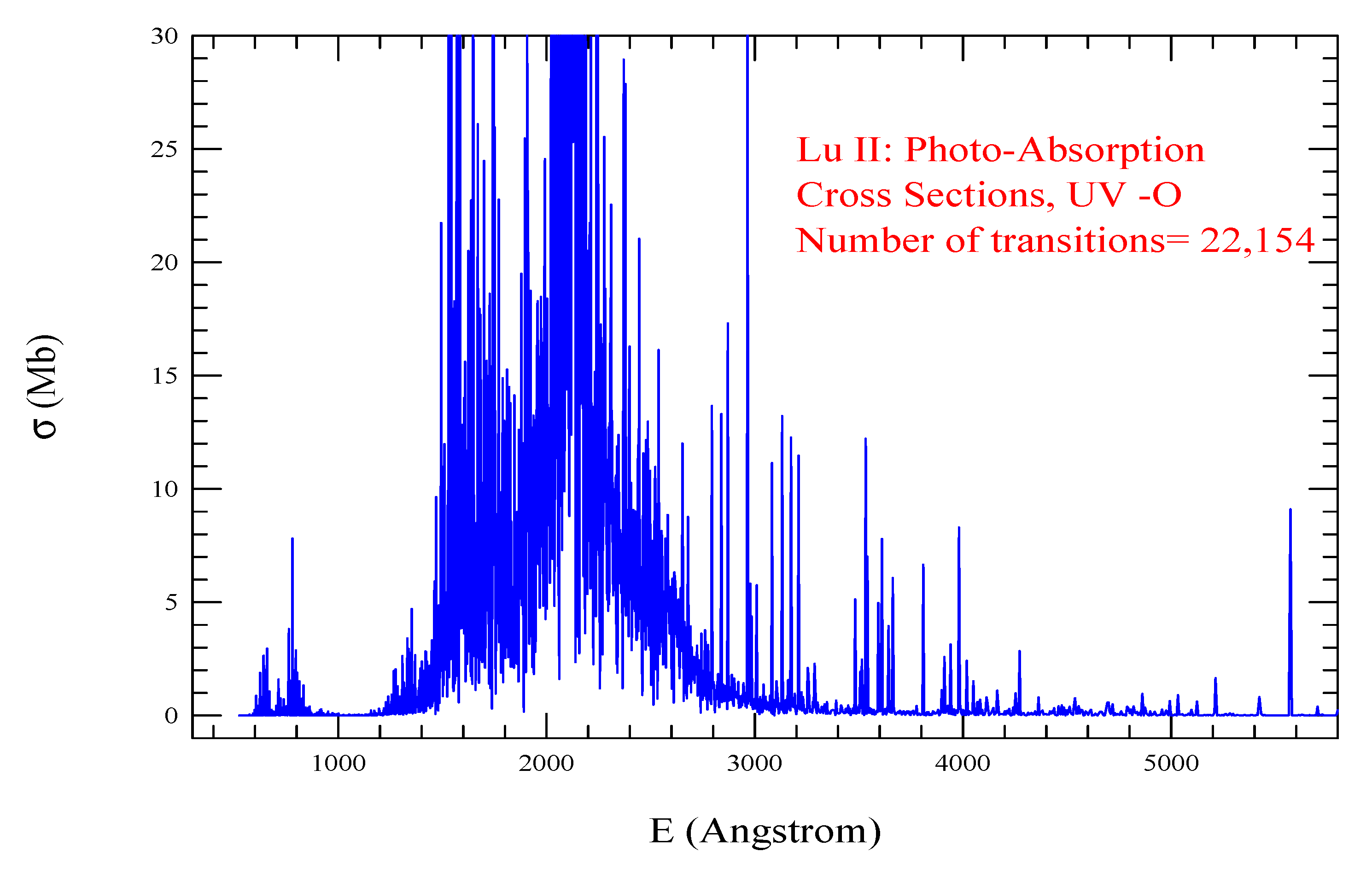
The photoabsorption spectrum ($\sigma$) of Lu II, presented in Figure 21, shows prominent lines in the energy region of UV to O. It has a wide broad region of strong photoabsorption lines in UV from 1400 to 2700 Å, with a dip around 1900 Å in the UV range. The number of transitions included is 22,142.

The photoabsorption cross-sections ($\sigma$) of Lu III, presented in Figure 22, show only a few strong lines. The number of transitions included is 159.

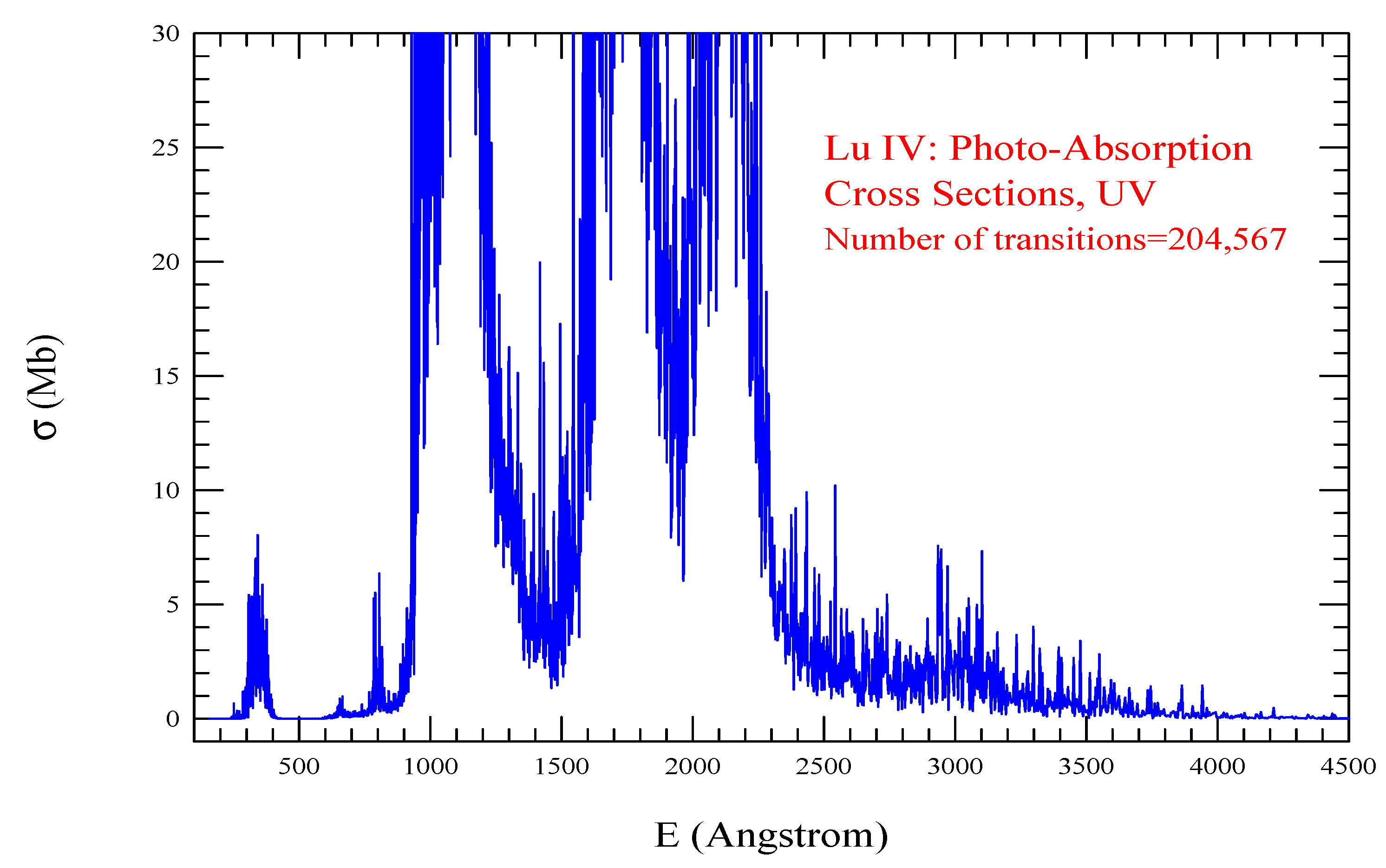
The photoabsorption cross-sections ($\sigma$) of Lu IV, presented in Figure 23, show the prominence of lines in the UV region. There are multiple broad absorption bumps in the spectrum. The number of transitions included is 204,567.

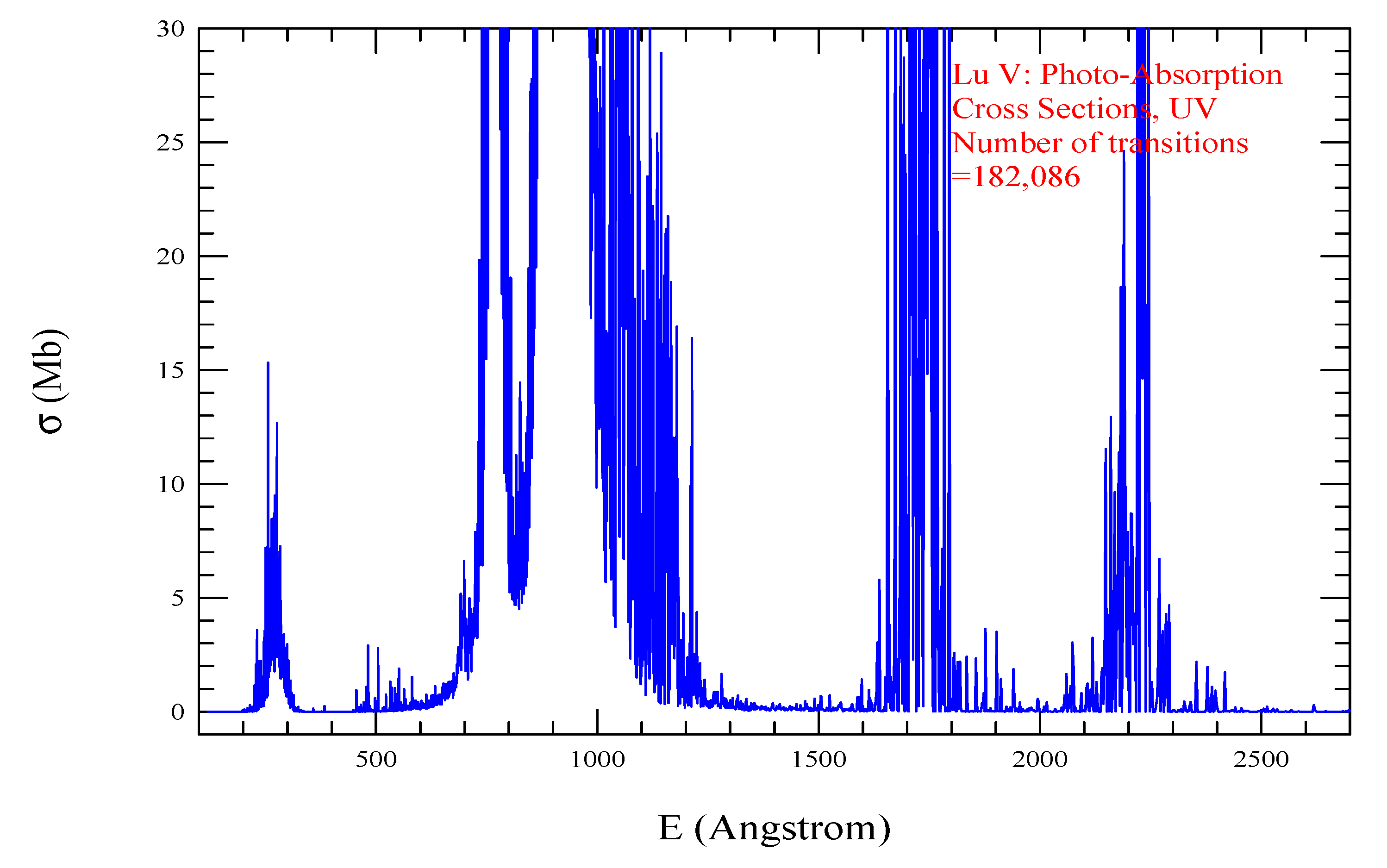
The photoabsorption cross-sections ($\sigma$) of the Lu V, presented in Figure 24, show the prominence of lines in the UV region. There are multiple broad absorption bumps in the spectrum. The broadest one is in the EUV range of 700–1200 Å with a dip at around 800Å. The number of transitions included is 182,086.

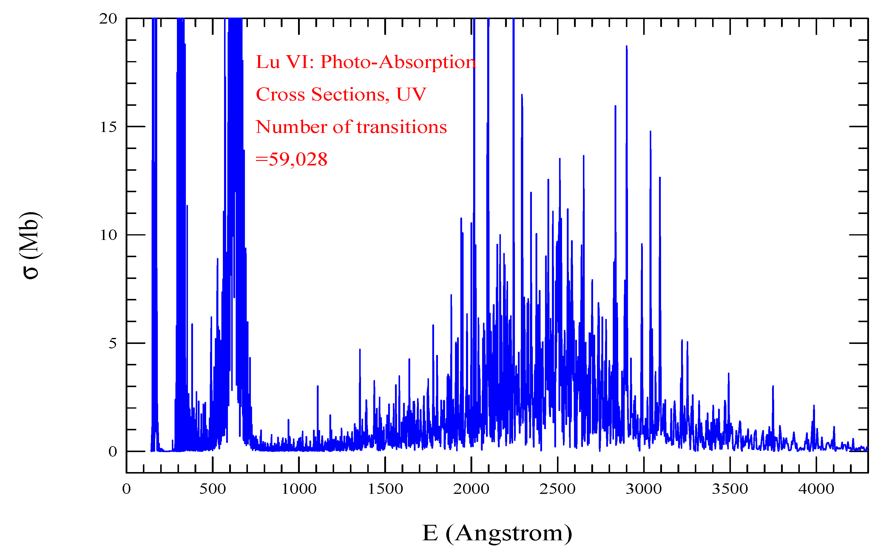
The photoabsorption cross sections ($\sigma$) of Lu VI, presented in Figure 25, show the prominence of strong lines from EUV to the near-O region. The spectrum shows three energy regions of very strong lines in the EUV range and a relatively broad feature at about 1700–3500 Å. The number of transitions included is 59,028.

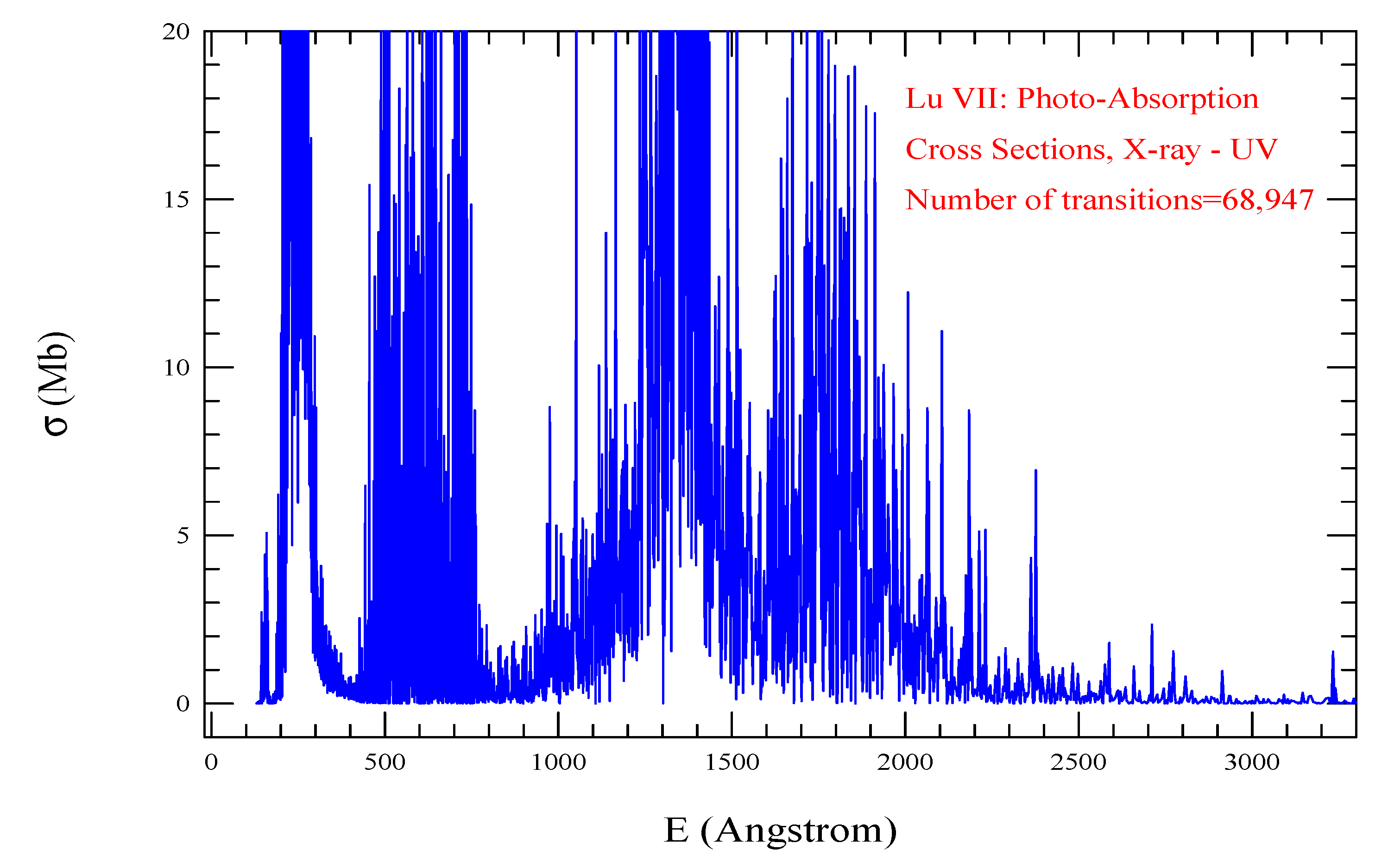
The photoabsorption cross-sections ($\sigma$) of Lu VII, presented in Figure 26, show the prominence of lines from EUV to UV. The spectrum shows multiple broad absorption energy bumps in the energy region. Two large absorption bumps are seen next to each other, covering an energy width of about 1000–2200 Å. The number of transitions included is 68,947.

The lanthanide ions described in the present report, with strong lines forming spectral features in the wavelength range of about 3000 to about 7000 Å, are the possible ion contributors of the broad feature of GW170817. It is also possible that ions with features in the UV range near 3000 Å and in the IR range beyond 7000 Å also make contributions but are not noticeable for reasons such as weaker transitions, the Doppler shift of the wavelengths, and shifts due to energy loss due to the opacity, which indicates absorption in the medium that the radiation passes through.

5. Conclusions

We summarize the present report as follows.

• We present atomic data for the energy levels and radiative transitions of 25 ions of lanthanides, Ho I-II, Er I-IV, Tu I-V, Yb I-VI, and Lu I-VII. Compared to the available datasets, these are probably the largest sets of atomic data for these lanthanide ions and can be applied for broad features, such as those from kilonovae events.
• These data, as extensive sets, are expected to be much more accurate than those available and hence should enable higher-precision astrophysical applications in broad features and fill the gaps in data needed for modeling. It should also be noted that the improved accuracy varies according to how the ion has been represented in the present study.
• The calculated energies have been benchmarked with the measured values, largely from Martin et al. [12], available on the NIST webpage [13]. The comparison shows overall good agreement, within a few percent, to fair to poor agreement, where the difference can be a factor close to 2 for the energies. This difference increases with higher energies.
• The radiative transition probabilities have been compared with those available at NIST [13], compiled from a number of sources. The agreement is fair to good. One factor in the differences is the proper identification of the levels. Much greater improvements will be needed over the present work for line diagnostic applications, using programs such as GRASP, which can provide limited but more accurate energies and transition parameters.
• We present the spectral features of these 25 lanthanide ions that illustrate the dominance of lines in various regions from X-ray to infrared.
• Very good agreement with the observed features in Figure 1 is found when compared with the calculated spectral features of Ho II. The observed features were generated by the photoabsorption of Ho II as the Ho compound was fragmented. The agreement is very good given given the strong electron–electron correlation interaction of a large atomic system like Ho II.
• Lanthanides have highly mixed levels and are very sensitive to slight changes in the representation of the potential and wavefunctions. These characteristics can lead easily to different sets of levels. Hence, guidance through experimentally determined levels is of great need and importance.
• All atomic data will be available online at the NORAD-Atomic-Data database (https://norad.astronomy.osu.edu, accessed on 7 July 2007) [25].

References

- Abbott, B.P.; Abbott, R.; Abbott, T.D.; Acernese, F.; Ackley, K.; Adams, C.; Adams, T.; Addesso, P.; Adhikari, R.X.; Adya, V.B.; et al. GW170817: Observation of Gravitational Waves from a Binary Neutron Star Inspiral. Phys. Rev. Lett. 2017, 119, 161101. [Google Scholar] [CrossRef]
- Pian, E.; D’Avanzo, P.; Benetti, S.; Branchesi, M.; Brocato, E.; Campana, S.; Cappellaro, E.; Covino, S.; D’Elia, V.; Fynbo, J.P.U.; et al. Spectroscopic identification of r-process nucleosynthesis in a double neutron-star merger. Nature 2017, 551, 67. [Google Scholar] [CrossRef]
- Kasen, D.; Badnell, N.R.; Barnes, J. Opacities and spectra of the r-process ejecta from neutron star mergers. Astrophys. J. 2013, 774, 25. [Google Scholar] [CrossRef]
- Tanaka, M.; Hotokezaka, K. Radiative transfer simulations of neutron star merger ejecta. Astrophys. J. 2013, 775, 113. [Google Scholar] [CrossRef]
- Tanaka, M.; Kato, D.; Gaigalas, G.; Kawaguchi, K. Systematic opacity calculations for kilonovae. Mon. Not. R. Astron. Soc. 2020, 496, 1369–1392. [Google Scholar] [CrossRef]
- Tanaka, M.; Kato, D.; Gaigalas, G.; Rynkun, P.; Radžiūtė, L.; Wanajo, S.; Sekiguchi, Y.; Nakamura, N.; Tanuma, H.; Murakami, I.; et al. Properties of Kilonovae from Dynamical and Post-merger Ejecta of Neutron Star Mergers. Astrophys. J. 2018, 852, 109. [Google Scholar]
- Radžiūtė, L.; Gaigalas, G.; Kato, D.; Rynkun, P.; Tanaka, M. Extended Calculations of Energy Levels and Transition Rates for Singly Ionized Lanthanide Elements. I. Pr–Gd. Astrophys. J. Suppl. Ser. 2020, 248, 17. [Google Scholar] [CrossRef]
- Fontes, C.J.; Fryer, C.L.; Hungerford, A.L.; Wollaeger, R.T.; Korobkin, O. A line-binned treatment of opacities for the spectra and light curves from neutron star mergers. Mon. Not. R. Astron. Soc. 2020, 493, 4143. [Google Scholar] [CrossRef]
- Cowan, R. The Theory of Atomic Structure and Spectra; University of California Press: Berkeley, CA, USA, 1981. [Google Scholar]
- Johnson, J.A. Populating the periodic table: Nucleosynthesis of the elements. Science 2019, 363, 474–478. [Google Scholar]
- Kobayashi, C.; Karakas, A.I.; Lugaro, M. The Origin of Elements from Carbon to Uranium. Astrophys. J. 2020, 900, 179. [Google Scholar] [CrossRef]
- Martin, W.C.; Zalubas, R.; Hagan, L. NSRDS-NBS 60; National Standard Reference Data Series; National Bureau of Standards: Washington, DC, USA, 1978; 422p. [Google Scholar] [CrossRef]
- Kramida, A.; Ralchenko, Y.; Reader, J.; NIST; ASD Team. NIST Atomic Spectra Database (Ver. 5.8). 2020. Available online: https://physics.nist.gov/PhysRefData/ASD/levels_form.htm (accessed on 1 January 1996).
- Carlson, T.A.; Nestor, C.W., Jr.; Wasserman, N.; McDowell, J.D. Calculated ionization potentials for multiply charged ions. At. Data Nucl. Data Tables 1970, 2, 63–99. [Google Scholar] [CrossRef]
- Meggers, W.F.; Corliss, C.H.; Scribner, B.F. National Bureau of Standards Monograph 145; National Bureau of Standards: Washington, DC, USA, 1975; 600p. [Google Scholar] [CrossRef]
- Morton, D.C. Atomic data for resonance absorption lines. II. wavelengths longward of the lyman limit for heavy elements. Astrophys. J. Suppl. Ser. 2000, 130, 403–436, Erratum in 2001, 132, 411. [Google Scholar] [CrossRef]
- Komarovskii, V.A. Oscillator strength for spectral lines and probabilities of electron transitions in atoms and single charged ions of lantanides. Opt. Spektrosk. 1991, 71, 559–592. [Google Scholar]
- Wickliffe, M.E.; Lawler, J.E. Atomic transition probabilities for Tm I and Tm II. J. Opt. Soc. Am. B 1997, 14, 737–753. [Google Scholar] [CrossRef]
- Sugar, J.; Meggers, W.F.; Camus, P. Spectrum and energy levels of neutral thulium. J. Res. Natl. Bur. Stand. Sect. A 1973, 77, 1–43. [Google Scholar] [CrossRef] [PubMed]
- Penkin, N.P.; Komarovskii, V.A.J. Oscillator strengths of spectral lines and lifetimes of atoms of rare earth elements with unfilled 4f-shell. Quant. Spectrosc. Radiat. Transf. 1976, 16, 217–252. (In Russian) [Google Scholar]
- Fedchak, J.A.; Den Hartog, E.A.; Lawler, J.E.; Palmeri, P.; Quinet, P.; Biémont, E. Experimental and theoretical radiative lifetimes, branching fractions, and oscillator strengths for Lu I and experimental lifetimes for Lu II and Lu III. Astrophys. J. 2000, 542, 1109–1118. [Google Scholar]
- Irvine, S.; Andrews, H.; Myhre, K.; Coble, J. Radiative transition probabilities of neutral and singly ionized rare earth elements (La, Ce, Pr, Nd, Sm, Gd, Tb, Dy, Ho, Er, Tm, Yb, Lu) estimated by laser-induced breakdown spectroscopy. J. Quant. Spectrosc. Radiat. Transf. 2023, 297, 108486. [Google Scholar] [CrossRef]
- Obaid, R.; Xiong, H.; Ablikim, U.; Augustin, S.; Schnorr, K.; Battistoni, A.; Wolf, T.; Carroll, A.M.; Bilodeau, R.; Osipov, T.; et al. In Proceedings of the 47th Annual Meeting of the APS Division of Atomic, Molecular and Optical Physics (DAMOP) Annual Meeting. Providence, RI, USA, 23–27 May 2016. Abstract: B9.00007. [Google Scholar]
- Pradhan, A.K.; Nahar, S.N. Atomic Astrophysics and Spectroscopy; Cambridge University Press: Cambridge, UK, 2011. [Google Scholar]
- Nahar, S.N. Database NORAD-Atomic-Data for atomic processes in plasma. Atoms 2020, 8, 68. [Google Scholar] [CrossRef]
- Nahar, S.N.; Eissner, W.; Chen, G.X.; Pradhan, A.K. Atomic data from the Iron Project–LIII. Relativistic allowed and forbidden transition probabilities for Fe XVII. Astron. Astrophys. 2003, 408, 789–801. [Google Scholar] [CrossRef]
- Eissner, W.; Jones, M.; Nussbaumer, H. Techniques for the calculation of atomic structures and radiative data including relativistic corrections. Comput. Phys. Commun. 1974, 8, 270–306. [Google Scholar] [CrossRef]
- Eissner, W. Atomic structure calculations in Breit-Pauli approximation. In The Effects of Relativity on Atoms, Molecules, and the Solid State; Wilson, S., Grant, I.P., Gyorffy, B.L., Eds.; Plenum Press: New York, NY, USA, 1991; pp. 55–64. [Google Scholar]
- Nahar, S.N. Atomic data from the Iron Project. Astron. Astrophys. 2004, 413, 779. [Google Scholar]
- Nahar, S.N. Modern Trends in Physics Research. In Proceedings of the 4th International Conference on MTPR-10, Sharm El Sheikh, Egypt, 12–16 December 2010; El Nadi, L., Ed.; World Scientific: Singapore, 2013; pp. 275–285. [Google Scholar]
Figure 1.
Photoabsorption cross-sections () of Ho II. Top: Experimental photoabsorption spectrum (black dashed curve) of Ho [23]. Bottom: Predicted spectrum of Ho II from the present work. The predicted energy is shifted by about 10 eV. Arrows point to energies E = 155, 160, and 180 eV, around which a change in feature in the measured spectrum is noticeable. The similarities in the features indicate that the black curve in the top panel corresponds to the photoabsorption features of Ho II following the fragmentation of Ho.
Figure 2.
Photoabsorption cross-sections () of Ho I demonstrating broad spectral feature in the UV wavelength region of 800–1150 Å.
Figure 3.
Photoabsorption cross-sections () of Ho II demonstrating broad spectral feature in the UV wavelength region.
Figure 4.
Photoabsorption cross-sections () of Ho III demonstrating a very broad spectral feature in the O–IR wavelength region, particularly ranging from 4000 to 15,500 Å.
Figure 5.
Photoabsorption cross-sections () of Er I demonstrating one broad, 1000–3500 Å, and one very broad, 4000–13,200 Å, spectral feature in the O–IR wavelength region.
Figure 6.
Photoabsorption cross-sections () of Er II demonstrating two broad spectral features in the UV (2200 Å)–near-optical (4000 Å) region.
Figure 7.
Photoabsorption cross-sections () of Er III demonstrating three regions of high peak strong lines from X-ray to UV regions: the first one is in the narrow X-ray region (around 80 Å), one is a relatively narrow region in the EUV range (300–500 Å), and one is a relatively large broad spectral region in the UV range (900–1700 Å).
Figure 8.
Photoabsorption cross-sections () of Er IV demonstrating multiple regions of high peak strong lines in the UV region.
Figure 9.
Photoabsorption cross-sections () of Tm I demonstrating three regions of high peak strong lines: one in the EUV region of 500–1500 Å, the second one in 1700–2500 Å, and the third one in the narrow band around 3400 Å. Noticeable lines become more sparse with larger wavelengths.
Figure 10.
Photoabsorption cross-sections () of Tm II demonstrating the visible presence of strong lines in the UV and IR regions and almost no strong lines in the optical (4000–7000 Å) region. Compared to other lanthanides discussed here, this ion has a smaller number of transitions and a relatively wider broad feature exists in the IR region.
Figure 11.
Photoabsorption cross-sections () of Tm III demonstrating multiple broad structures from EUV to O wavelength range, with the widest one being in the range of 1200–2500 Å.
Figure 12.
Photoabsorption cross-sections () of Tm IV. There are four distinct broad regions, with strong lines, in the wavelength regions from EUV up to UV.
Figure 13.
Photoabsorption cross-sections () of Tm V in the energy range of EUV to UV. It demonstrates multiple broad structures from the EUV to the UV wavelength range, with the widest one being in the range of 1400–1900 Å with a dip at around 1650 Å.
Figure 14.
Photoabsorption cross-sections () of Yb I in the energy range of UV to O. A region of strong lines appears in the wavelength range of about 2600–3500 Å.
Figure 15.
Photoabsorption cross-sections () of Yb II with dominating strong lines in the energy range of EUV–UV. The spectrum shows two broad features, one in the wavelength range of 1500–2100 Å and another one in 2500–3100 Å.
Figure 16.
Photoabsorption cross-sections () of Yb III in the energy range of EUV to O. The spectrum has multiple broad features dominated by strong lines in the energy range of EUV–O. The strongest absorption bump is in the wavelength range of 2200–3000 Å.
Figure 17.
Photoabsorption cross-sections () of Yb IV in the energy range of E to EUV to UV, exhibiting multiple regions of strong lines.
Figure 18.
Photoabsorption cross-sections () of Yb V in the energy range of E to EUV to UV. It has two broad features dominated by strong lines: one in the EUV region followed by a lower peak structure and a broader absorption bump in the wavelength region of 1600–2500 Å.
Figure 19.
Photoabsorption cross-sections () of Yb VI in the energy range of UV. It has two absorption bumps next to each other in the energy range of 145–170 Å.
Figure 20.
Photoabsorption cross-sections () of Lu I in the energy range of UV–IR, showing several energy regions of strong lines.
Figure 21.
Photoabsorption cross-sections () of Lu II in the energy range of UV–O. Prominent lines are seen in the energy region from UV to O. The spectrum has a wide broad region of strong photoabsorption lines in UV ranging from 1400 to 3300 Å.
Figure 22.
Photoabsorption cross-sections () of Lu III in the energy range of UV. The spectrum has only a few strong lines.
Figure 23.
Photoabsorption cross-sections () of Lu IV in the energy range of UV, showing multiple absorption bumps in the UV region.
Figure 24.
Photoabsorption cross-sections () of Lu V with prominent lines in the UV energy region. The spectrum shows the presence of multiple broad photoabsorption bumps. The broadest one is in the EUV range of 700–1200 Å with a dip around 800 Å.
Figure 25.
Photoabsorption cross-sections () of Lu VI showing the presence of strong lines in the energy region from EUV to near O. The spectrum shows 3 energy regions of very strong lines in the EUV range and a relatively broad feature at about 1700–3500 Å.
Figure 26.
Photoabsorption cross-sections () of Lu VII with prominent absorption lines in the energy range of EUV–UV. The spectrum shows multiple broad absorption energy bumps in the energy region. The prominence of strong lines in the absorption bumps, one from 150 Å in the X-ray range to 350 Å in the EUV range and one from 400–800 Å in UV, can be seen. Two absorption bumps exist next to each, covering a energy width of about 1000 to 2200 Å.