Laser and Astrophysical Plasmas and Analogy between Similar Instabilities

Abstract

Multipulse laser–matter interactions initiate nonlinear and nonequilibrium plasma fluid flow dynamics and their instability creating microscale vortex filaments, loop-soliton chains, and helically paired structures, similar to those at the astrophysical mega scale. We show that the equation with the Hasimoto structure describes both, the creation of loop solitons by torsion of vortex filaments and the creation of solitons by helical winding of magnetic field lines in the Crab Nebula. Our experiments demonstrate that the breakup of the loop solitons creates vortex rings with (i) quasistatic toroidal Kelvin waves and (ii) parametric oscillatory modes—i.e., with the hierarchical instability order. For the first time, we show that the same hierarchical instability at the micro- and the megascale establishes the conceptual frame for their unique classification based on the hierarchical order of Bessel functions. Present findings reveal that conditions created in the laser-target regions of a high filament density lead to their collective behavior and formation of helically paired and filament-braided “complexes”. We also show, for the first time, that morphological and topological characteristics of the filament-bundle “complexes” with the loop solitons indicate the analogy between similar laser-induced plasma instabilities and those of the Crab and Double-Helix Nebulas—thus enabling conceptualization of fundamental characteristics. These results reveal that the same rotating metric accommodates the complexity of the instabilities of helical filaments, vortex rings, and filament jets in the plasmatic micro- and megascale astrophysical objects.

1. Introduction

Many physical problems—like the plasma system dynamics and instability—are complex in nature and include various physical processes, taking place on a wide range of space and time scales. Their effects on plasma dynamics occur at the time scales from nanoseconds to several millennia and at the spatial scales from less than a micron to those measured in the light years. As mechanisms occur on different scales to the patterns they shape, this makes scale the key conceptual problem in the evolution of shock-induced flow in the plasmatic systems [1,2,3,4,5]. Having established a relationship between the physical processes that govern plasma dynamics and the evolution of instabilities at the laboratory microscale, one can establish an analogy with the processes at a much larger scale of astrophysical objects, like Nebulas. Reflecting on experiences from studying laser–matter interactions (LMIs) and plasmatic systems at various scales, it is possible to conclude that there are some common features (a common “skeleton” in the multidisciplinary research—relating to multiphysics phenomena) [5], but that, each system will have its specific differences.

In this paper, we aim to give an overview of the main characteristics of plasma systems created by intense and ultraintense lasers, which cause plasma instabilities and structures generated by the shock-induced variable density flow and by the magnetohydrodynamic-induced instabilities.

The first part of this article summarizes features with regard to the (i) main characteristics of laser-generated plasmas by intense lasers (≥10⁸ W/cm²) and ultraintense lasers (≥10¹⁵ W/cm²) [2,3,4,6]; (ii) the physical processes that can be initiated at these power densities; and (iii) characteristics of laser-generated plasma instabilities, which are analyzed having in mind that similar phenomena occur in the astrophysical systems like stars and nebulas. Along this line of thinking, the conceptualization of fundamental characteristics of laser-induced plasma instabilities is extended and applied to those observed in the Crab Nebula and Double-Helix Nebula.

2. Short Outlines of Plasmas Generated by Intense and Ultraintense Lasers

2.1. Plasmas Created by Intense Lasers

Plasma formation in laser–matter interaction (LMI) is initiated when the laser power density reaches the optical breakdown threshold, which depends on the laser pulse (energy, wavelength, and pulse duration) and the target material (optical, thermal, and electrical properties and surface morphology). The early stages of plasma evolution created by intense power lasers of the pulse duration τ~10⁻⁹ s and power density ~10⁸–10¹¹ W/cm² are characterized by the high electron density (~10¹⁹cm⁻³) and temperature ~10⁴ K [7,8], which may reach ~10⁵ K, and dominated by the Bremsstrahlung continuum emission [9]. Both the electron density and temperature decrease with time due to plasma spheroid expansion and recombination phenomena. High collision frequency between the free electrons and heavy species (atoms and ions) leads to excitation/de-excitation and ionization/recombination equilibria [9].

Regarding this process, the excited ions and atoms in the laser-induced plasma soon de-excite by emitting radiation; atomic line emission forms the “laser-induced breakdown signal”, which enables spectroscopic diagnostics. The line emission—superimposed on the continuum emission—can be observed after the plasma expansion associated with the fast decrease in temperature [9]. Plasma spheroid evolution/expansion depends on the energy deposited into the target, as well as on the environmental conditions (vacuum or background gas).

In the vacuum environment, plasma spheroid evolution is adiabatic and depends on the laser pulse duration; it is therefore different for the ns, ps, and fs laser pulses. According to [10], laser pulses longer than about 5ps cause the laser–plasma interaction and plasma heating with the temperature increasing with pulse duration, which is well illustrated for the ns pulses. “Due to the fact that the electron-lattice heating time is ~10⁻¹² s, which is ~1000 times shorter than the pulse duration—the ns-laser pulse causes domination of thermal effects over the ionization. The laser pulse melts and vaporizes target surface, while the temperature increase ionizes the atoms. The plasma spheroid becomes opaque for laser radiation between 10⁻⁹ s and 10⁻⁸ s, so that the tail of the laser pulse interacts with the plasma spheroid becoming absorbed. The absorbed nanosecond laser pulse causes plasma reheating, elongates its lifetime, increases line emission, but also increases the background emission” [10].

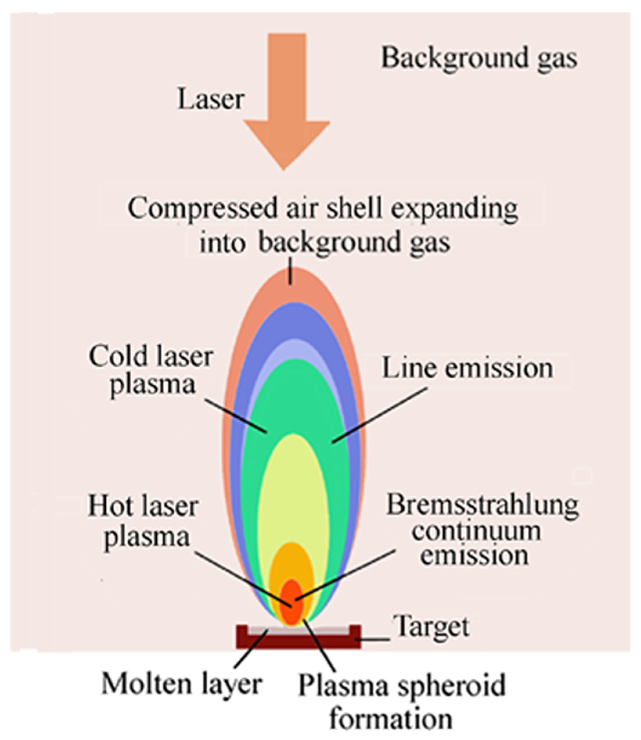
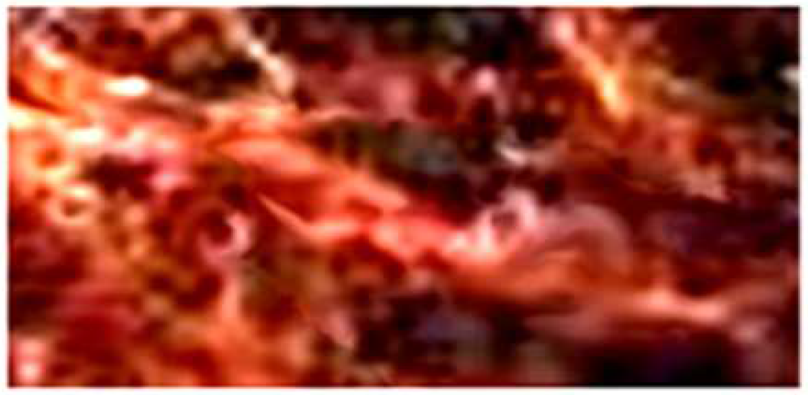
In the background gas environment, plasma spheroid evolution is non-adiabatic and depends on ablated mass, spot size, energy deposited into the target, and the pressure of background gas. Plasma creation and evolution in the background gas are shown in Figure 1.

Characteristics of plasma evolution also depend on the laser pulse duration and the wavelength. Considering the ns-LMIs and the wavelengths ranging from the far infrared CO₂ laser (λ = 10.8 μm, τ = 100 ns), to the infrared Nd–YAG laser (λ = 1.06 μm, τ = 40 ns), to the visible Ruby laser (τ = 30 ns, λ = 600 nm),and to the ultraviolet XeCl laser (λ = 308 nm, τ = 16–20 ns), one finds that in all cases plasma expansion depends on the interaction with the surrounding background gas [11,12]. The expanding plasma becomes a mixture of atoms and ions of both, vaporized target material (In, Co, Fe, Ti, etc.), and ambient gas. The reaction with components of the background gas (usually air) like O₂ and CO₂ generates metal-oxide molecules, etc., as ionized species. Its lifetime—depending on density, the ambient gas, and the laser wavelength—ranges from ~300 ns to >40 μs [9].

For dependence of the plasma lifetime on the wavelength, it was found that short-wavelength UV irradiation of the iron target creates plasma, which is initially dominated by the continuum background up to ~400 ns; then, the atomic line emission appears and extends to the μs time scale. The longer wavelength of an IR laser causes the continuum emission at longer times ranging to several microseconds [9]. The evolution of the line emission intensity for two iron lines (Fe I 285.2 nm and Fe II 288.4 nm) shows characteristic behavior. During the first 3 μs, the intensity of the ionic line exceeds the neutral atoms by 50 times, whereas after ~10 μs, the neutral line intensity increases and becomes eight times that of the ionic [9].

The dependence of the plasma lifetime on the pressure of the background gas can be related to the expansion velocity—as observed from the ICCD (intensity field charge-coupled device) photographs of visible emission and the size of the aluminum plasma cloud. For the pressure of p = 100 Tor~1.33 × 10⁴ Pa [13], it was found that the initial expansion velocity of ~3000–4000 m/s—(between 450 ns and 950 ns after the plasma formation)starts to decrease after ~1500 ns to ~900–1000 m/s. This continues to ~2000 ns (2 μs) when the light emission ends. However, for the atmospheric pressure p = 10⁵ Pa, the expansion velocity is lower while the plasma lifetime is extended for a few orders of magnitude. For the giant laser pulses, the plasma lifetime extends to ~0.2 ms [14]. In general, characteristics of laser-induced plasma change with time and with the spheroid expansion, between ns and μs time scale, when the plasma spheroid extends over the target surface [10].

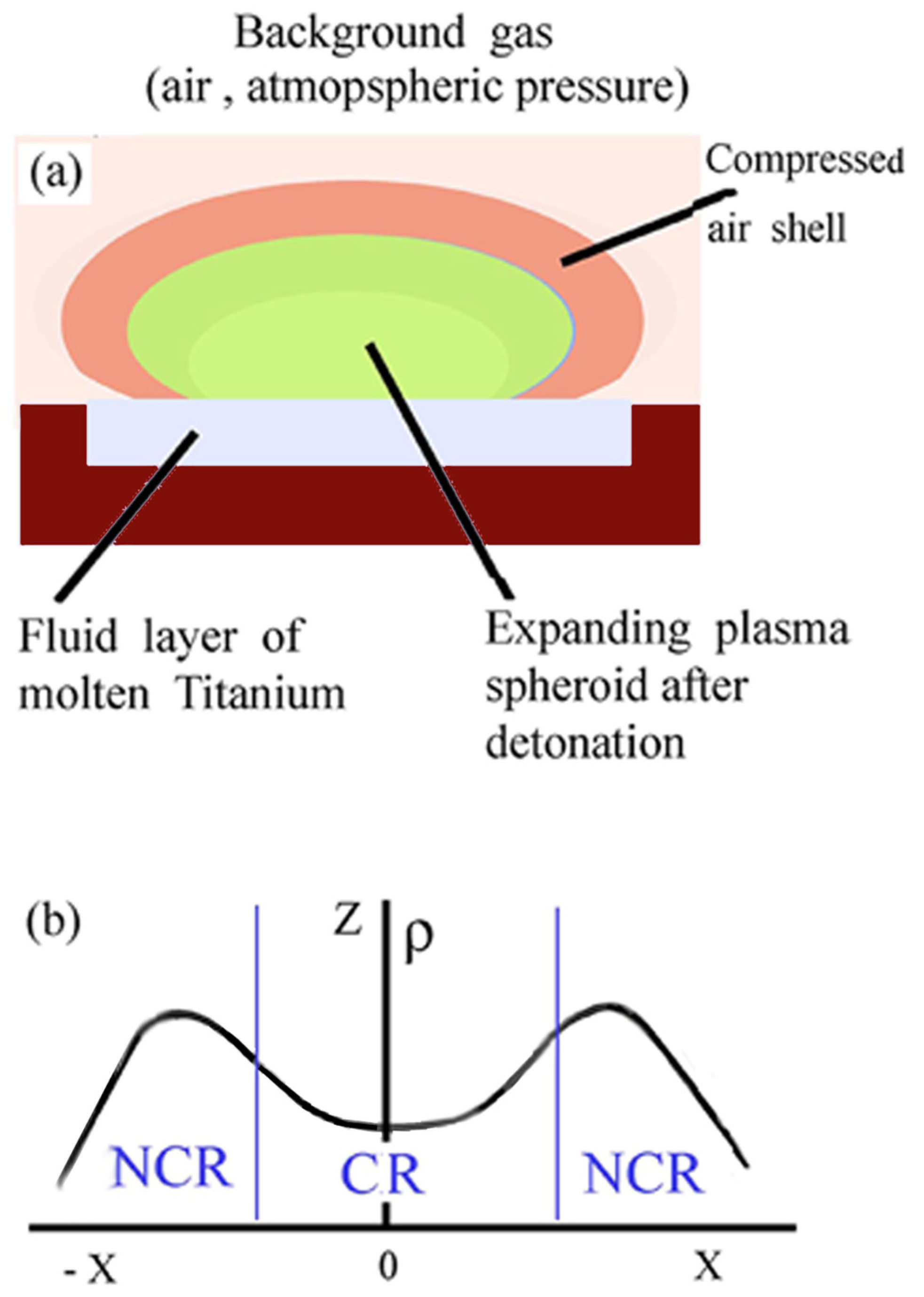
Expansion of the plasma spheroid into the surrounding background gas forms the air shell [15] or the cocoon [16,17,18,19] (Figure 2a). With the expansion, its density decreases in the central region (CR) and increases at the periphery of the spot (in the NCR and NPR), resulting in the inversion of the initial density profile. Radial differences in the plasma density may become very large. The number density of the light-fluid particles in the NCR is higher for about two orders of magnitude with respect to the CR as shown in [15,20]. Figure 2b shows the cross-section of the expanding plasma spheroid in the (z,x) plane.

Plasma-generated shock with “blast profile” or simply called blast wave “is a shock wave that consists of a leading shock front followed by expansion wave which decays its strength at a steady rate. This decay occurs across all the properties behind the leading shock. For a typical shock wave with ‘step profile’ or ‘shock profile’, the properties behind the shock remain constant” [21]. The shock wave striking density interface of the vapor/plasma (low-density fluid, (ρL) and molten surface layer (high-density fluid, (ρH)) impulsively accelerates the light fluid into the heavy fluid causing the evolution of instabilities due to the transfer of mass, momentum, and energy to the density interface.

The pressure shock generated in the confined (or semiconfined) configuration may be estimated as follows [22]. Assuming the laser power density of ~1 GW/cm² (which is higher than the plasma breakdown threshold of various metals of ~0.36 GW/cm² according to [23]), the plasma detonation generates a shock wave with the pressure peak p(kbar), given by the Raizer equation [22,24,25].

$$p=0.1\sqrt{\frac{aZI}{2a+3}}$$

(1)

where Z is the reduced shock impedance of the two materials, I is the flux of the laser beam (GW/cm²), and $a$ is the corrective factor, $a\approx 0.20$, and Z~390,625 (~4 × 10⁵) [22].

Estimation of the pressure generated in the confined configuration for the laser power density, I ~ 1 GW/cm², and $a$ and Z parameters similar to Devaux et al. [22], Equation (1) is as follows [17]:

p~15.3 kbar~1.53 GPa.

(2)

Detonation of plasma discoid in a spatially localized laser-heated region causes the overpressure within a background gas. However, the overpressure quickly diminishes, and the vapor/plasma blast wave is highly accelerated [26].

Impulsive fluid acceleration by the shock wave causes Richtmyer–Meshkov instability (RMI) as a vorticity-driven phenomenon, which starts with linear growth as small amplitude perturbations. It evolves with time when the incident shock wave propagates from a light to a heavy gas $(\nabla p .\nabla \rho <0)$ or from a heavy to a light fluid $(\nabla p .\nabla \rho >0)$, associated with phase reversal [27,28,29,30,31,32]. The instability causes perturbation on the interface to grow, producing vortical structures followed by the generation of bubbles and spikes. According to Schiling and Jacobs [32], «after passage of a shock wave—the interface begins to decelerate. The pressure behind the shock front decreases monotonically with distance, so that the reversal of pressure and of density gradients occurs from the heavy into the light fluid».

Rayleigh–Taylor instability (RTI) is initiated with the constant acceleration by the shock wave of the heavy fluid into the lighter one, when the density gradient is mismatched with the direction of the acceleration, i.e., $(\nabla p .\nabla \rho <0)$. The interaction of a pressure gradient ($\nabla p$, from shock) with a misaligned density gradient ($\nabla \rho$, from the interface) causes the evolution of the vorticity caused by the baroclinic torque at the interface of the fluid with the velocity $\upsilon$. The deposition of baroclinic vorticity on the density interface can be described by the dynamics of the vorticity field $(\mathbf{\omega }=\nabla \times \upsilon )$[28,31,32,33,34]. The baroclinic vorticity deposition by the shock wave is governed by the 3D vorticity equation:

$$D\omega /Dt=(\nabla \rho \times \nabla p)/{\rho }^2+\mathbf{\omega }\cdot \nabla \mathbf{\upsilon }-\mathbf{\omega }(\nabla \mathbf{\upsilon })$$

(3)

where $D/Dt=\partial /\partial t+\mathbf{\upsilon }\nabla$, and $(\nabla \rho \times \nabla p)/{\rho }^2$ is the baroclinic term, $\mathbf{\omega }\cdot \nabla \mathbf{\upsilon }$ is vortex stretching and $\mathbf{\omega }(\nabla \mathbf{\upsilon })$ is vortex dilatation [31,32,33]. The amount of vorticity deposition increases with the increase in density gradients (Atwood number), pressure gradients (shock strength or Mach number, Ma), and the mismatch angle α between the pressure and density gradients (as sinα) [27].

The perturbations of the density interface start to grow into spikes of heavy fluid into light fluid and bubbles of light fluid into heavy fluid, generating the Rayleigh–Taylor instability [33,34,35]. The subsequent shear flow along the growing spikes causes Kelvin–Helmholtz (KH) instability and the formation of mushroom-shaped caps at the RTI spikes [17,18,19,36]. The key parameter governing the instability is the shock Mach number, Ma, which determines the effects of compressibility in the flow. It means that for weak shocks, the fluid dynamics may be described as assuming incompressible flow [32].

In many studies, the assumption is that the shock-induced fluid acceleration is stationary in space-time; in that case, the energy transfer is Kolmogorov direct cascade characteristic for the isotropic homogenous turbulence. However, in a more general case, the acceleration may be variable (nonstationary), leading to different RMI and RTI dynamics and non-Kolmogorov inverse cascade [37,38,39,40]. The variable acceleration is assumed to be a power law function of time, $g=G{t}^a$, t > 0, where a is the exponent of an acceleration power law, a ∈ (−∞, +∞), and G is the pre-factor, G > 0, and their dimensions are $\left[G\right]=m/s^{2+a}$ and [a] = 1. The evolution of instability is considered on the fluid layer with the periodic flow in the plane (x,y) normal to the z direction of the acceleration g; ∣g∣ = g, and also the acceleration directed from the heavy to the light fluid, g = (0,0,−g) along the z-axis [39,40,41]. The evolution of RMI/RTI starts from infinitesimal spatial perturbations at the density interface, governed by parameters like the initial perturbation (the height of the disturbance h and the wavelength, Λ of parallel scratches on modulated target surface), the Atwood number A, $A=({\rho }_H-{\rho }_L)/({\rho }_H+{\rho }_L)$, and the momentum transfer.

Initial perturbation conditions: The initial perturbation—which on metal targets is deposited by the set of parallel scratches—creates multimodal perturbation. Becoming the seed of interface instability, this perturbation initiates the growth of RMI/RTI at early times and depends on the amplitude and wavelength of the perturbation modes. The multimode perturbation is the basis of the interference concept of the RMI and RTI evolution. This concept—besides the amplitude and the wavelength—also takes into account the phase relations between the modes that lead to interference of the initial perturbation modes [42,43].

The laser-generated shock wave moving on the scratched target surface becomes dispersed into a fast oscillatory wave and a slow modulation wave [44]. Thus, the shock and reshock waves in the fluid layer become oscillatory waves with variations in the phase and amplitude, wavelength and frequency, as well as the direction of propagation. When such oscillatory shock wave strikes the density interface, it causes fluid acceleration and shock-induced variable density flow with the formation of RTI as well as the shear layer roll-up into vortex filaments if the Re number is Re > Re_crit.

2.2. Plasmas Created by Ultraintense Power Lasers

Ultraintense power lasers create plasmas with extremely high electron density and temperature as well as strong magnetic and electric fields. A high degree of ionization, high velocities, high density, and pressure in such plasmas are comparable to that in the laser-induced inertial confinement fusion and in the stars. This makes it possible to establish an inter-relationship between laboratory, magnetic fusion, inertial fusion plasma, space, and astrophysical experiments [2,3,4,5,45], as the high energy density phenomena. In this respect, it should be noticed that “a significant fraction of the visible Universe is composed by matter in extreme conditions of temperature, density and pressure. When the pressure in a physical system exceeds 1 Mbar, this is defined as a high energy density (HED) state, which corresponds to the pressure required to deform the water molecule or in other words the pressure at which water becomes compressible, corresponding to an energy density exceeding 10¹¹ J/m³…” [46].

Creating such plasmas, lasers of the power density from 10¹⁸ W/cm² [46] up to 10²⁴ W/cm², with the pulse duration of τ < 10⁻⁹ s (ns)–10⁻¹² s (ps) and to 10⁻¹⁵ s (fs) make possible the study of matter under extreme conditions by monitoring the light emission, the emission of the X-rays and plasma debris. In the plasmas created by intensities of ~10¹⁴ W/cm², laser fields start to compete with intra-atomic fields, causing rapid ionization and complex dynamics of the electron wave function [6]. An example is lithium plasma created by the ultrashort pulse of τ = 10⁻¹² s, of 2 × 10¹⁵ W/cm², with the electron temperature of 35 eV (4 × 10⁵ K) and high electron density of ~10²¹ cm⁻³ showing the soft X-ray emission between λ = 1 nm and 15 nm [47]. A linear increase in the Li III Ly_α- and Ly_β-line intensity coincides with the plasma expansion length. For the higher intensity of ~10¹⁶ W/cm², the laser fields surpass the intra-atomic fields that band electrons and enable rapid ionization of various targets. At even higher intensities of ~10²³ W/cm², plasma manifests the new phenomenon: individual incoherent emission (radiation damping) of electrons which start to affect the plasma dynamics suppressing the plasma instabilities. This causes an energy transformation into the gamma range and the emission of gamma radiation [6].

Dynamics of plasmas created by ultraintense lasers are intended to mimic plasma dynamics in cosmic explosions and planetary cores creating ultrahigh-pressure shocks [47] In this respect, irradiation of a small sphere by an ultraintense laser creates intense shock waves and ultrahigh pressures reaching ~10¹² atmospheres. Such gigantic shock fronts are similar to the thin shock regions at the boundary between a collapsed supernova and the surrounding material—creating a spheroid of super-hot plasma. Its hot steep front is associated with a turbulent magnetic field, which affects plasma behavior [48].

Magnetic fields in laser plasma are self-generated fields caused by direct laser acceleration [49] and driven by intense and ultraintense laser pulses. They vary in strength, topology, and timescale over many orders of magnitude [50]. Laser-generated magnetized plasma can be scaled to astrophysical plasmas. A 0.5–2 kJ laser with a pulse duration of 1 ns creates a laser plasma and fast electrons that induce a current in the coil generating a magnetic field [50]. Their strength ranges from 50–200 T [51,52], to 600–800 T [53,54], and even to the tens of kilotesla [46,55].

A kilotesla strength magnetic field was generated by fs ultraintense laser pulses of P = 65 TW and I ≈ 10²⁰ W/cm² [56]. The strength of such a magnetic field can be estimated by considering the absorption rate of the laser beam:

$$a_{abs}=n_{\mathrm{e}}/2n_{\mathrm{c}}c\tau .$$

(4)

where c is the speed of light, and τ is the pulse duration; they used the model valid for low-order orbital angular momentum (OAM) modes, characterized by the parameters ℓ and σ_z. Parameter ℓ relates to the order of azimuthal modes, while σ_z is the spin number; ${\sigma }_z=\left[\pm 1\right]$ denotes a circularly polarized beam, and σ_z = 0 denotes a linearly polarized beam. For the fs pulse and multi-terawatt laser power and given electron plasma density n_e, the peak axial magnetic field strength of the modes $({\sigma }_z=1,l=0)$ and $({\sigma }_z=0,l=1)$ is given by the relationship [56]:

$$|B{|}_{max}(\mathrm{KT})\approx 10\{P(\mathrm{TW}){\lambda }^3(\mu \mathrm{m})\}/{\mathrm{W}}_0^4(\mu \mathrm{m}).$$

(5)

For the laser plasma parameters n_e = 0.03_cr, beam wavelength λ = 1 μm, beam waist w₀ = 6 μm, $a_{abs}=0.435$ mm⁻¹, τ = 100 fs, and p = 65 TW, where n_c is the critical plasma density, Equation (5) gives the peak of the axial magnetic field strength of B = 1 kT. This kilotesla, multipicosecond, axial magnetic field was found to extend over hundreds of microns in underdense plasma [56].

In astrophysically relevant laser experiments, such strong magnetic fields are measured by proton imaging, in which high-energy protons interact with the electromagnetic fields, creating spatial variations in the proton fluence on the diagnostic plane [48]. The collisionless interaction of two counter-propagating, laser plasmas “results in the formation of small-scale magnetic filaments. This process created in the laboratory may explain the presence of magnetic fields throughout the intergalactic medium” [48]. Proton images that indicate the amplitude of the field and its orientation relative to a proton’s trajectory display features corresponding to the magnetized filaments and reveal randomized systems of filamentary magnetic fields [48]. Magnetic fields in laser plasmas are found universally in all plasma regimes from astrophysical to fusion systems [48,50]. While the magnetic fields govern the dynamics of plasma expansion and the evolution of plasma instabilities, very strong magnetic fields enhance the generation of ion beams; they affect the formation and propagation of plasma filament jets in nebulas.

3. Short Outlines of the Experiments

The experiments—shortly described below—have shown that various plasma flow instabilities can be created by laser–matter interaction, which on the metal targets stay permanently after pulse termination. Multipulse laser irradiation of metal surface modulated by parallel micro-scale scratches has been used in order to induce initial multimodal perturbation [12,57,58,59] Interference of the initial perturbation modes results in the evolution of various plasma flow instabilities on pure metal targets and targets coated by layers of different metal types. The Co-coated steel plate targets of 1 × 1 × 0.05 cm were exposed (in the open configuration) to the beam of XeCl excimer laser (λ = 308 nm, of E = 250–300 mJ, Es ~ 5 J/cm², I~2.4 × 10⁸ W/cm², τ ≤ 20 ns), of the rectangular cross-section with constant power density distribution (top hat profile), and irradiated by N = 12 pulses at the low repetition frequency of 10 Hz. Laser irradiation of the Co-coated steel plate from above in the air at the atmospheric pressure (p = 10⁵ Pa) generated a high-temperature plasma spheroid, which expanded laterally along the “cold” target surface as described above, establishing the surface shear layer. Nonlinear and nonequilibrium processes at the power density scale of ≥10⁸ W/cm² take place in the shear layer of the plasma/molten-target surface. Driven by the shock-induced variable density flow, these processes lead to the evolution of the Rayleigh–Taylor instability, vortex filaments, and filament loops. This is especially emphasized when the interaction occurs with multimodal surface perturbation when the interference of initial perturbation modes causes various flow instabilities and the formation of a number of fluid flow structures. Their relaxation time is longer than the liquid-layer solidification time, so that they solidify ultrafast after pulse termination and become “imprinted” in the surface morphology. The cooling interval of ~5 ns or longer is comparable to the heating time, while the cooling rate is ~10⁹–10¹⁰ K/s [12]. The structures—permanently solidified—make possible a posteriori analysis. Thus, the target surface represents a “diagnostic plane” for the interface dynamics. The structures “encoded” in the surface morphology represent time integrated picture of hydrodynamic instabilities. A posteriori optical, SEM, and AFM analysis enables the identification of characteristic RMI and RTI structures, the vortex filaments and jets, their wavelength, and amplitude, as well as their organization and symmetry.

4. Results and Discussion

4.1. Vortex Filament Formation in Laser Plasma

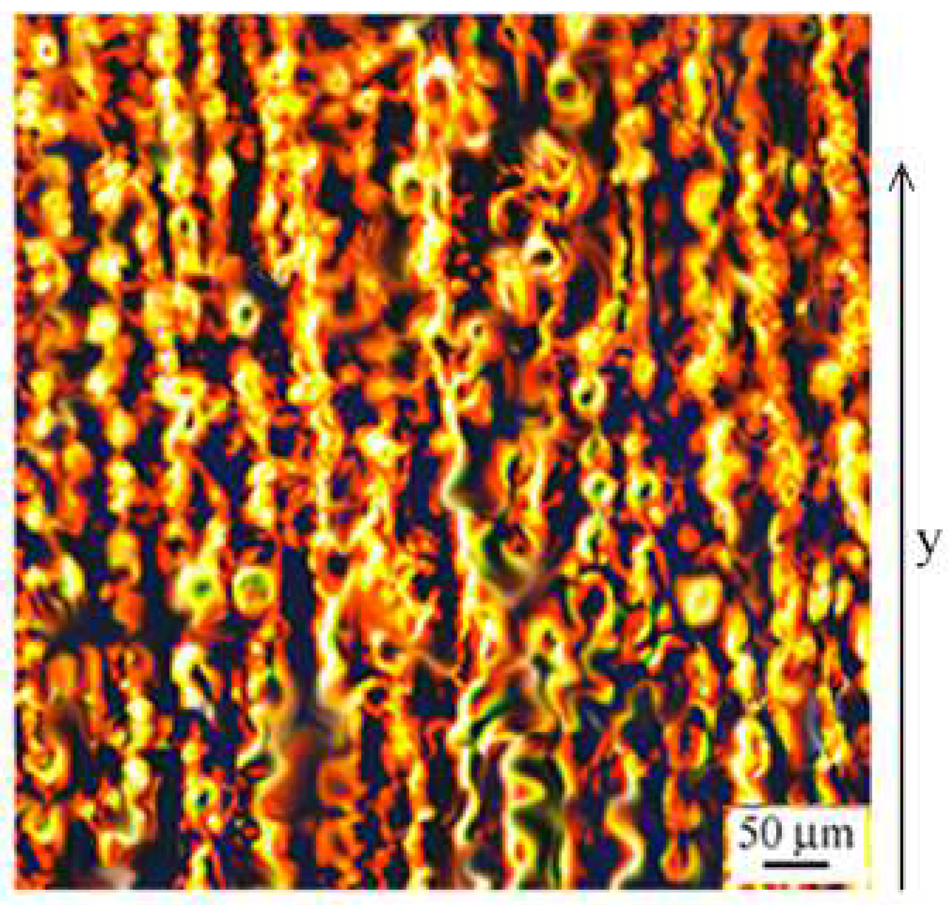
The shock wave acceleration of the shear layer (variable density flow) establishes the RT environment and causes the rollup of shear waves into a series of parallel micron-scale vortex filaments and wave–vortex structures. Their formation on the target surface was promoted by the parallel micron-scale scratches (with the separation distance Λ, which causes transversal perturbation of the shock wave as $\Psi =\mathrm{A}exp(k_{p}x)$, where A is the perturbation amplitude equivalent to the height of the scratch wall, and k_p is the perturbation wave vector; $k_p=2\pi /\Lambda (\mu {\mathrm{m}}^{-1})$. An oscillatory shock perturbs the shear layer transversally to the y-direction, causing the formation of waves and their roll-up into vortex filaments; their length reaches L ≳ 500 μm, while the core thickness is about σ ~5–7 μm [57,58,59,60,61,62] (Figure 3).

Surface patterning and multipulse LMI create a series of shock waves of different wavevectors, phases, and intensities. Two kinds of vortex filament arrays are formed; the low-density one, in which the filament–filament distance, Λ is much larger than the core size σ $(\Lambda >>\sigma )$, and a high-density array $(\Lambda \le \sigma )$. The parameter Λ is a crucial parameter that determines whether the filaments in the array will manifest individual dynamics after N pulses, or they will interact and form secondary coherent structures like thick-vortex filaments, ribbons, vortex filament-bundles, and braided and tangled structures [61].

4.1.1. Individual Dynamics of Vortex Filaments

Vortex filaments formed with a large separation distance, Λ ≳ 10 μm (a 1D vortex-filament lattice), extend in the y-direction on the target surface and manifest individual behavior. Their formation on the surface shear layer can be described by two dynamically important quantities; the square of the vorticity modulus [63] is as follows:

$${\omega }^2=1/2{\Sigma }_{\mathrm{i}\mathrm{j}}{({\mathsf{\partial }}_{\mathrm{i}}{\mathrm{u}}_{\mathrm{j}}-{\mathsf{\partial }}_{\mathrm{j}}{u}_{\mathrm{i}})}^2$$

(6)

and the square of the rate of strain tensor [64] is as follows:

$$T^2=1/2{\Sigma }_{\mathrm{i}\mathrm{j}}{({\mathsf{\partial }}_{\mathrm{i}}{u}_{\mathrm{j}}+{\mathsf{\partial }}_{\mathrm{j}}{u}_{\mathrm{i}})}^2$$

(7)

The latter quantity is linked to the local energy dissipation $\epsilon =\nu T^2\rho$, where ρ is the fluid density, and ν is the kinematic viscosity. Another quantity connected with the above two is the pressure field p, which can be written [63] as follows:

$$\Delta p=(\rho /2)({\omega }^2-T^2)$$

(8)

The regions of the shear layer with large ω² and small $T^2$ become rolled up into vortex filaments. Namely, the horizontal shock-momentum component causes acceleration of the shear layer, while the vertical one causes Kelvin–Helmholtz instability and rollup into axisymmetric vortex filaments when the Reynolds number Re ≥ Re_critical [63].

The velocity field of the vortex filament in the cylindrical coordinates, $U=U(u_r,u_{\nu ,}{u}_{\Theta })$, has the components: $u_z=\gamma z$ (γ = strain), and $u_{\Theta }=\Gamma /2\pi r(1-\exp (-\gamma r^2/4\nu ))$ where ν = kinematic viscosity and Γ is the circulation. The Gaussian vorticity distribution across the filament is [63] as follows:

$$\omega (r,t)=\Gamma /4\pi r(\exp (-\gamma r^2/4\nu ))$$

(9)

The fluid velocity $U$ is comparable with the velocity of the expelled vapor of ~10³–10⁴ m/s. Assuming $U$~5 × 10³ m/s, the kinematic viscosity of liquid metal, ν~10⁻⁶ m²/s, and the thickness h of the molten layer is h~(1–2) × 10⁻⁶ m, one finds the Reynolds number $\mathrm{Re}=Uh/\nu \approx 5\times 10^3$ to be 10⁴. At some places, a plasma cloud of ~10⁴–10⁵ K is created above the liquefied-boiling surface (T_B~2–5 × 10³ K), associated with high fluid velocity, and the critical Re number for the formation of vortex filaments, estimated to be Re_crit~10⁴. For the filament of the core size, σ (σ = 2r₀~5–7 μm), the circulation, $\Gamma =2\pi \sigma U$, is Γ~0.3 m²/s. After formation, the vortex filament immersed in the background turbulent field starts to move on the surface.

4.1.2. Generation of Loop Solitons on Vortex Filaments

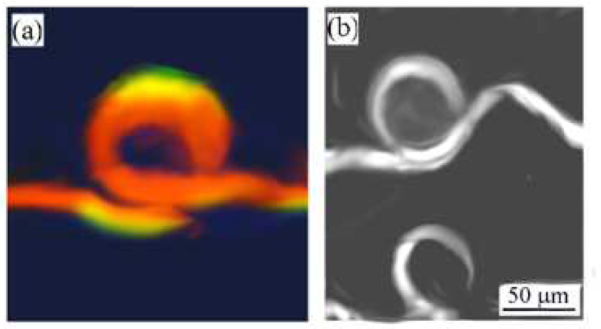
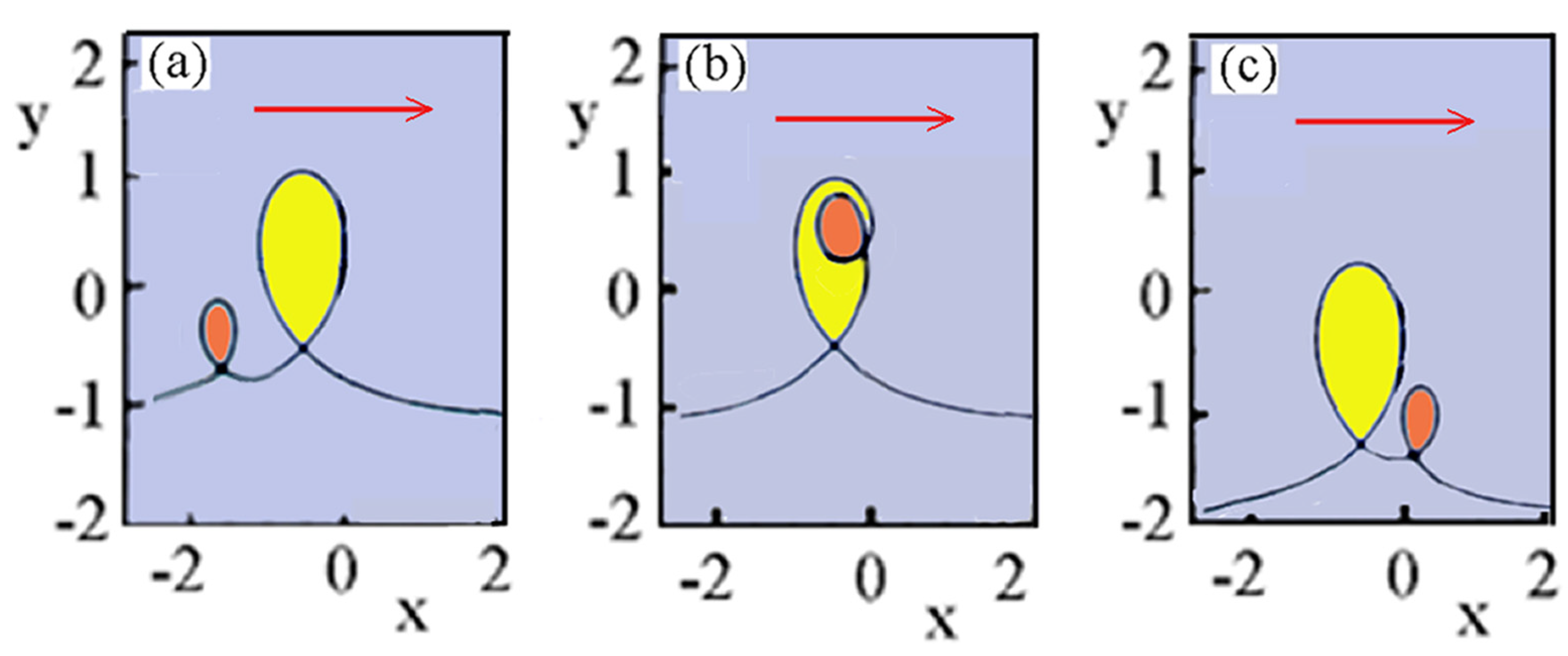
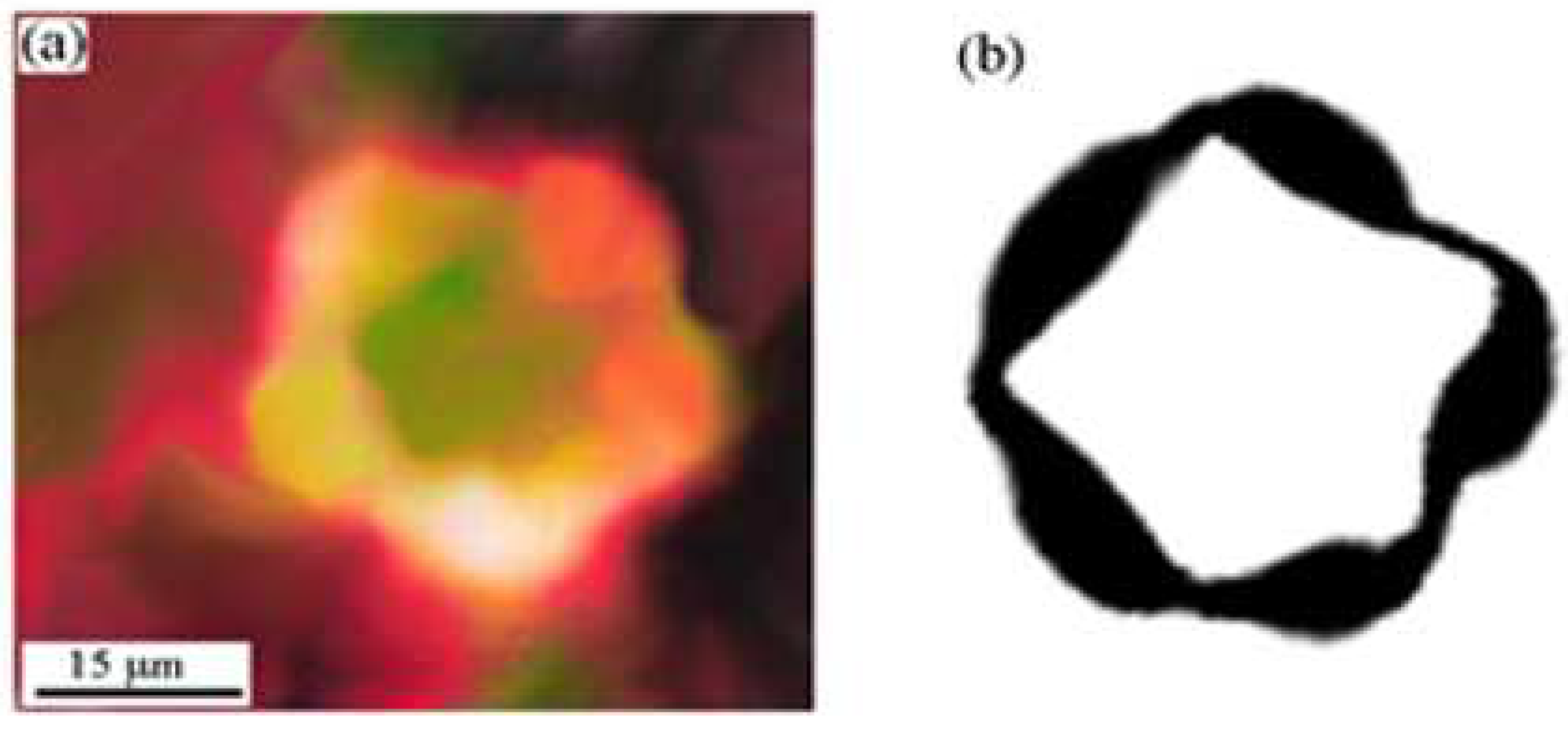
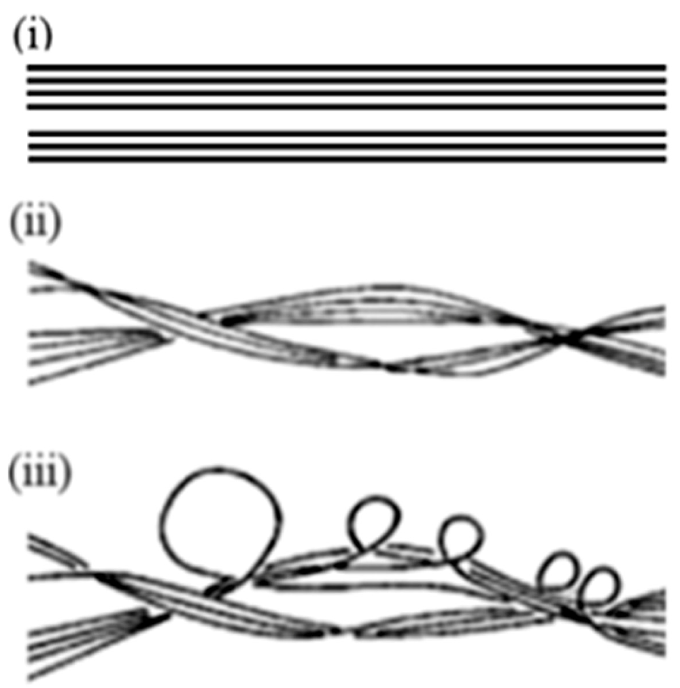
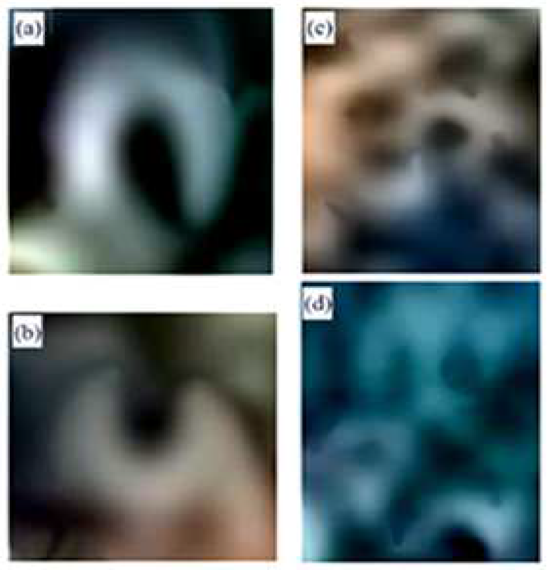
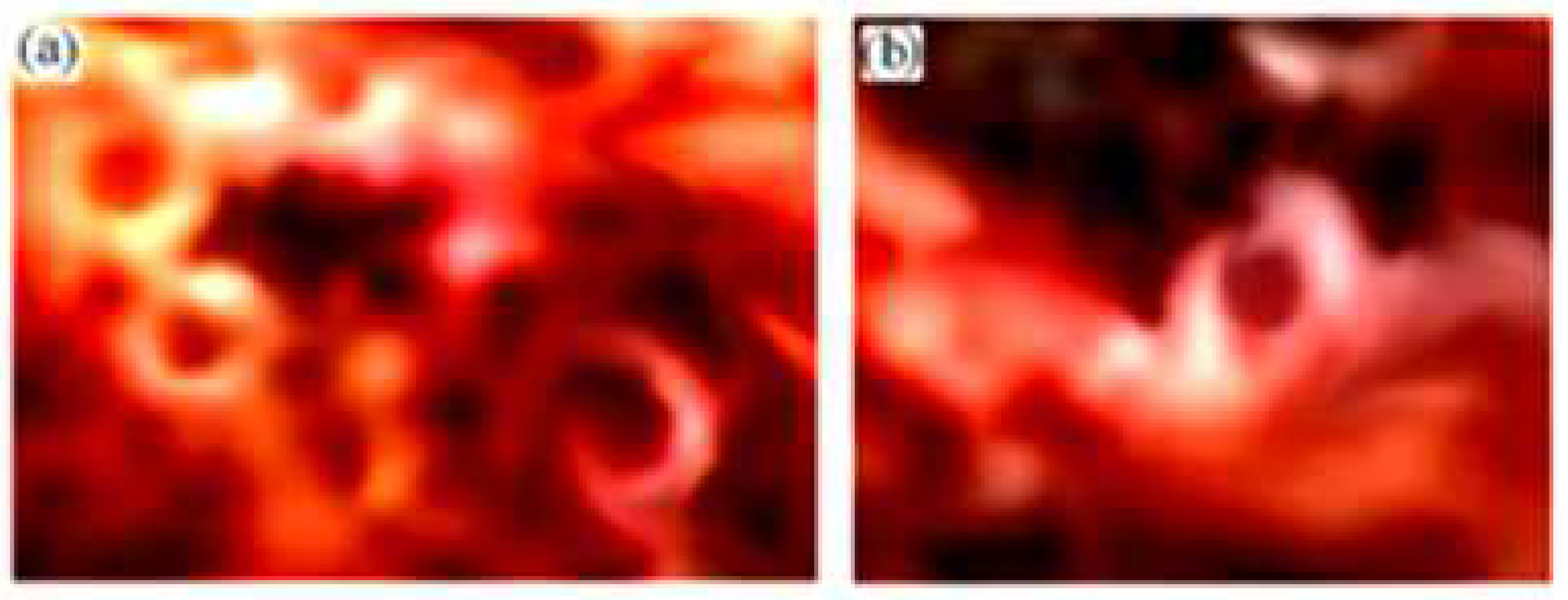
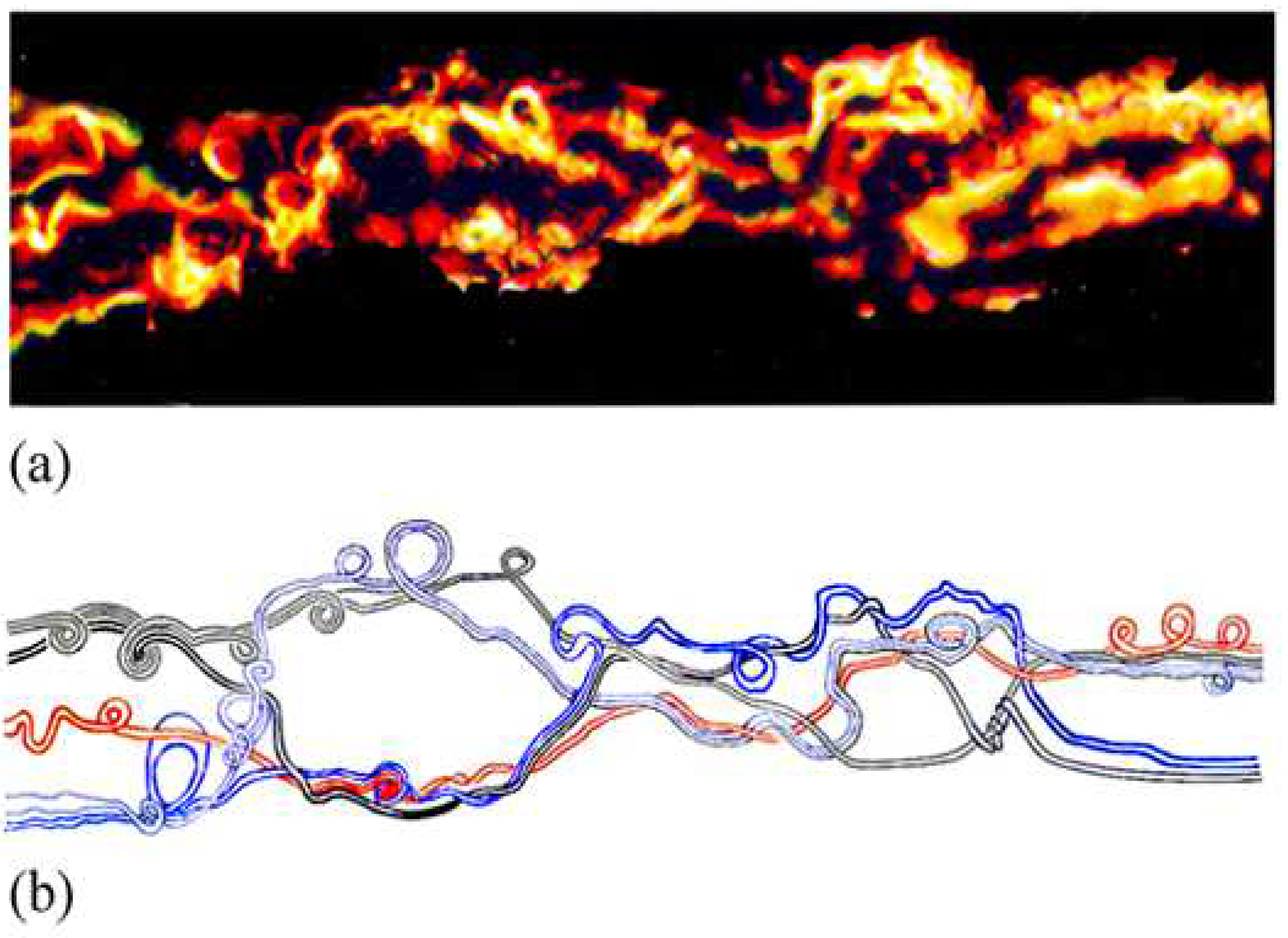
Motion of a vortex filament of the length L and the core diameter d immersed in an external flow U_ext (background turbulent shearing field) at any point is affected by its shape along its entire length. However, it is reasonable to expect that the contribution to the vortex velocity from distant parts of the filament is small compared to the local contributions [64]. The curvature of the vortex filament exposed to torsion due to interaction with a turbulent shearing field creates loops called the Hasimoto solitons [57,59,64] (Figure 4a,b).

If the diameter d of the filament does not change along the length L, the condition L/d = constant makes it possible to describe its motion by the localized induction approximation (LIA). The vortex filament experiences a self-induced velocity described by the equation of motion, i.e., by the LIE written as [57,59,64] follows:

$$\mathsf{\partial }x/\mathsf{\partial }t=Ck\mathit{b}+U_{ext}{\mathit{e}}_x, C=\Gamma /4\pi \ln (L/d)$$

(10)

where $k$ is the curvature of the filament curve, b the unit binormal vector, Γ the circulation of the vortex, and e_x is the unit vector in the x-direction.

The loop solitons may travel without friction along the filament and appear in LMI and in other systems including those at the astrophysical scale. For the loop soliton of the radius R, with d < R < L, the dynamics on filament can be described on the basis of LIA [57,58,59]. Neglecting the background flow, the nonlinear perturbations can be described by a coupled system of Betchov–Da Rios equations, written in terms of local curvature $k$ and torsion $T$. Using the complex function, $\Psi$ (the Hasimoto transformation) is as follows:

$$\Psi =kexp(i{\displaystyle \int Tds})$$

(11)

These equations are transformed into the non-linear Schrödinger equation:

$$(1/i)\mathsf{\partial }\Psi /\mathsf{\partial }t=\mathrm{C}\cdot \left[{\mathsf{\partial }}^2\Psi /\mathsf{\partial }{s}^2+(1/2)({\Psi }^2+\mathrm{A})\Psi \right]$$

(12)

where s is the arch length along the filament and A is an arbitrary function of time t. For a single-loop soliton, the curvature $k$ may be written [57,58,59] as follows:

$$k=2\eta \mathrm{sech}\left[\eta (s-2\mathrm{C}T\cdot t)\right]$$

(13)

where η is constant, the torsion $T$ and the velocity of the curvature (soliton loop) are constant.

The motion of the soliton loop along the filament can be studied as the traveling wave solution. For the reason of simplicity, we look for the traveling wave solution in 2D. Using a modified Korteveg de Vries (mKdV) equation, one finds a 2D solution for a planar curve [65,66]. The mKdV equation for the planar curvature k can be written as follows:

$$k^{,}+k^{,,,}+(\frac{3}{2})k^{,}{k}^2=0$$

(14)

with boundary conditions $k\to 0,\mathrm{s}\to \pm \infty$. The solution of the equation can be constructed by means of the symbolic programs based on the Hirota method [66,67] for the transformation of the mKdV equation into bilinear form, which is a complex procedure and out of the scope of this paper. Following the procedure of the Hirota method, one finds the curvature $k$ of the loop in 2D [66]

$$k=\left[2k\exp (\omega t+ks)\right]/\left[\exp (2\omega t)+\exp (2ks)\right]=2k\sec \Theta$$

(15)

where $\Theta =ks-\omega \mathrm{t}$, and dispersion $\omega =k^3$. After finding the radius of the loop, the solution of the equation yields the loop soliton as real and imaginary parts of the radius vector of the loop [66].

$$x(s,t)=s-\frac{2}{k}(\tanh \omega \mathrm{t}+\tanh \Theta )$$

(16)

$$y(s,t)=\frac{2}{k}(\mathrm{sech}\omega \mathrm{t}-\mathrm{sech}\Theta )$$

(17)

The loop soliton propagates with increasing time; its size decreases as the wave vector increases: Therefore, a smaller loop travels faster than a larger loop [66].

4.1.3. Loop Soliton Chain: Multisolitons

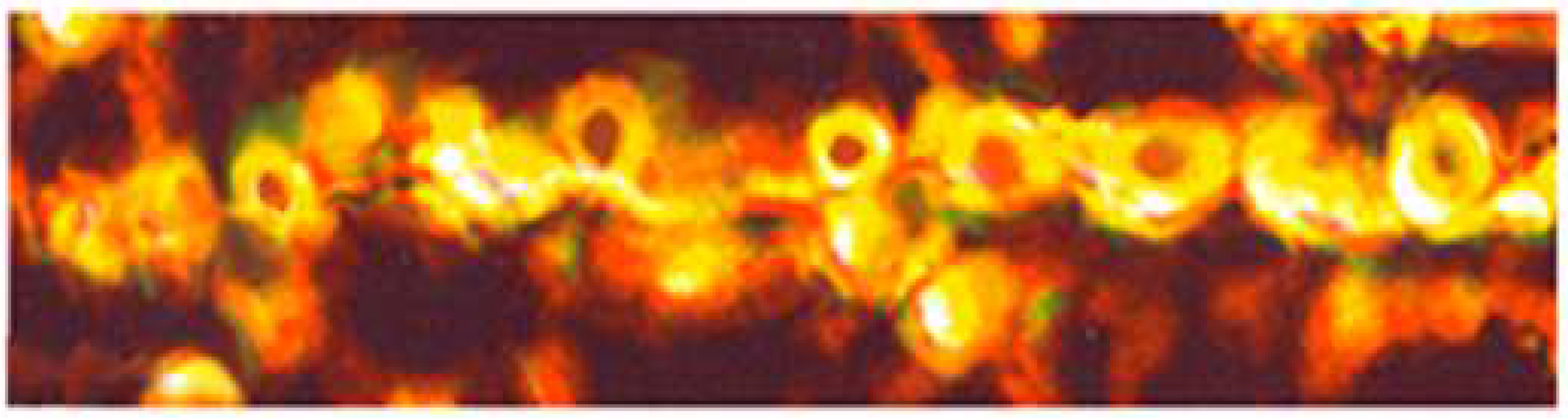
Multipulse laser–matter interactions with patterned target surfaces create a series of such loops—the loop-soliton chains on vortex filaments [57,58,59], as well as supercomplex 3D networks [61]. The loop-soliton chain—such as the one generated on the Co-coated steel, may be compared with the chain of particles—a 1D periodic lattice (Figure 5).

For a simple illustration of the multisoliton dynamics, we present the motion of 2D loop solitons of different radii r₁ and r₂, with the curvatures $k_1$ and $k_2$ [66]. The solution of the two loop solitons is obtained by the same Hirota transformation of the mKdV equation into bilinear form, as above, and the result is presented in Figure 6.

This figure shows the propagation of two solitons with $k_1=3$ and with $k_2=1$ in nondimensional time. Rather long expressions for $k_1$ and $k_2$ are obtained by very complex procedures, detailed in [66].

When a large number of almost parallel vortex filaments is generated, the loop soliton chains can be formed simultaneously on such an array. A quasi-linear array of parallel vortex filaments (which are slightly disturbed and make quasi-periodic 1D lattices) is created by multipulse LMI with Co-coated steel. In such an array of parallel vortex filaments, the multipulse LMI usually forms an inhomogeneous turbulent field, in which the torsion of vortex filaments $T$ may be small or large and may vary with the series of pulses. As a consequence, the solitons of different radii and curvatures $k_1$, $k_2$, … will be formed on the filaments. In the oscillatory strain field associated with multipulse LMI, the situation may be created in which torsion on some filament causes (+) and (–) curvature and the loop solitons, which may cancel each other or may form complex loop-soliton chains.

Such a complex case of parallel loop-soliton chains on vortex filaments is shown in Figure 7.

The radius of the loop solitons is R~25–30 μm, i.e., they are mostly of the same size, meaning that they travel almost at the same velocity. However, a slight difference in the loop size and curvature causes the solitons of smaller radius to travel faster than the larger ones. As a result, they approach their neighbor solitons and—an initially periodic 1D loop soliton lattice—becomes quasiperiodic (Figure 7).

Loop solitons and multiple loop solitons generated by laser plasma at the microscale represent mimics of similar megascale structures appearing in astrophysical plasma systems like nebulas, as will be shown for the Crab Nebula.

4.1.4. Breakdown of the Loop Soliton Chain: Generation of Vortex Rings and Vortex Ring Instability

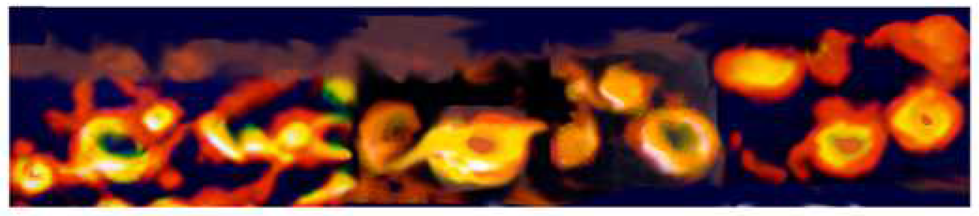
When the number of pulses reaches some critical level (N = Ncrit)—we show—consistent with our previous results [58] that LMI creates conditions that favor complex dynamics including a breakdown of the loop soliton lattice into individual open loops and vortex rings. After collapse-and-reconnection, the loop solitons become unstable and yield a cascade of vortex rings. Then, simultaneous excitation of spectra on vortex rings occurs due to perturbation by a random inhomogeneous strain field [58].

Such a scenario takes place for N ≳ 12, because pulsation causes the local strain field to become larger than the vorticity ω. Then, the strain field causes the collapse of the loops followed by reconnection, thus creating a cascade of vortex rings. They are further exposed to the straining fields and, in the cooling phase (at the end of every laser pulse), to the viscosity effect; after formation, rings practically do not move from the former position in the string, as seen in Figure 8.

Regarding the source of the strain field, it may be said that “The source of the strain field may be classified into three categories: (a) internal or self-induced strain, (b) mutually induced strain field by companion rings, (c) external strain, varying from place to place, imposed by the pressure field of a laser pulse” [58] Subsequently, random local multipolar strains excite the unstable waves on vortex rings, which cause instability with hierarchical order. On some vortex rings, new types of instabilities appear, which have not been observed previously or have been predicted only theoretically [58].

Considering the effect of the strain field on the vortex ring instability, one can assume that in the absence of external shear, asymptotic expansions of the Navier–Stokes equations for a vortex ring may be carried out for a small parameter, $\epsilon =\mathrm{a}/R$, where a and R are the core and the ring radius, respectively. Viewed locally, the leading-order flow represents a columnar vortex with a Gaussian vorticity distribution. The velocity field $V$ comprising radial, r, and azimuthal, $\Theta$, velocity components can be expanded as [58] follows:

$$V=V_0(r)+\epsilon V_1(r,\Theta )+{\epsilon }_2{V}_2(r,\Theta )+\dots \dots$$

(18)

where $V_0$ is the velocity component independent of $\Theta$. The field $V_1$ component comprises terms proportional to $\cos \Theta$ and $\sin \Theta$, while the quadrupole field $V_2$ comprises terms proportional to $\cos 2\Theta$ and $\sin 2\Theta$ [58] and causes deformation of the ring core into an elliptical shape; the associated instability, called elliptical instability, was discussed by Lugomer and Fukumoto [58], and references are cited there. In that case, the local strain fields—which have different symmetry properties—are arranged in increasing (higher) order, i.e., a dipole field, then a quadrupole field in second order and so on.

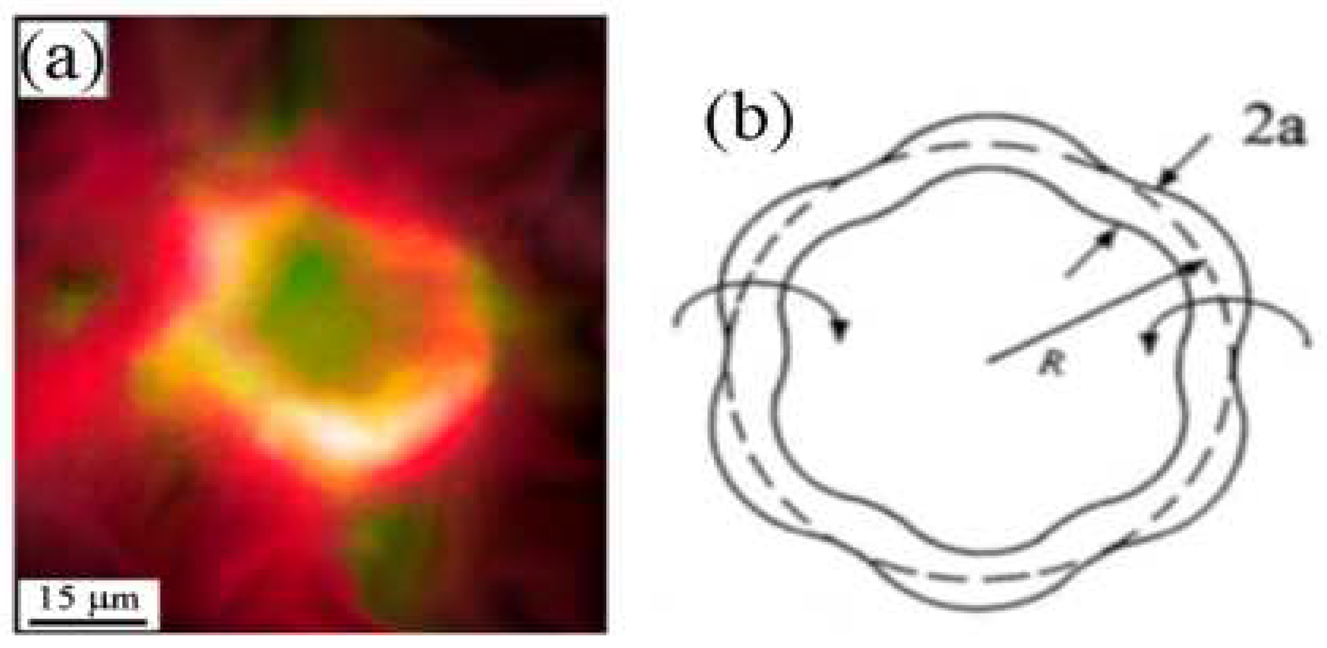
Assuming that the “vortex ring is separated by a few diameters from the mother filament, and the ring radius R is smaller than the distance to the filament, than the self-induced strain on a vortex ring outweighs the strain caused by neighbor filaments” [58]. In that case, the frozen pictures of a distorted vortex ring can be characterized by the instability of an isolated vortex ring. A simplified stability analysis of a vortex ring, chosen as $V_0$ the Rankine vortex (a circular cylindrical vortex of uniform core), revealed that the instability is a parametric resonance between a pair of Kelvin waves. The analysis also revealed that the quadrupole field $V_2$ supports the resonance between two helical waves. In general, the resonance instability is possible at frequency and wavenumber $k$ for which Kelvin waves with azimuthal wavenumbers m and m + 2 are simultaneously excited by disturbance υ₀ of the basic flow [58,68,69]:

$$v_0=\left[v_0(r){\mathrm{e}}^{im\Theta }+v_0^{(2)}(r){\mathrm{e}}^{i(m+2)\Theta }\right]{\mathrm{e}}^{i(ks-\omega t)}$$

(19)

where the arclength parameter s is taken along the center circle of the torus [70]. The major perturbation $V_1$ supports the resonance between pairs of Kelvin waves whose azimuthal wavenumbers differ by 1 [69,71]. Curvature instability is a parametric instability of vortex rings as found by [72]. Since the dipole field $V_1$ is tied with the vortex line curvature, this resonance is called curvature instability [68].

As shown in these laser experiments, even an isolated vortex ring can afford to accommodate a number of instability modes. Fukumoto made classification of the observed rings relies on the theories of parametric resonance and takes into account that long-wavelength oscillations on isolated vortex rings—in the laser experiment—are excited by the additional external straining field [58]. Namely, the multipulse LMI causes repetitive or time-periodic modulation of the multipolar strain field in the interaction space. “This modulation is different in different regions due to in-homogeneity in the distribution of local strain-field symmetry. As a consequence, various types of instability are created in different regions of the quasi-linear array of rings” [58].

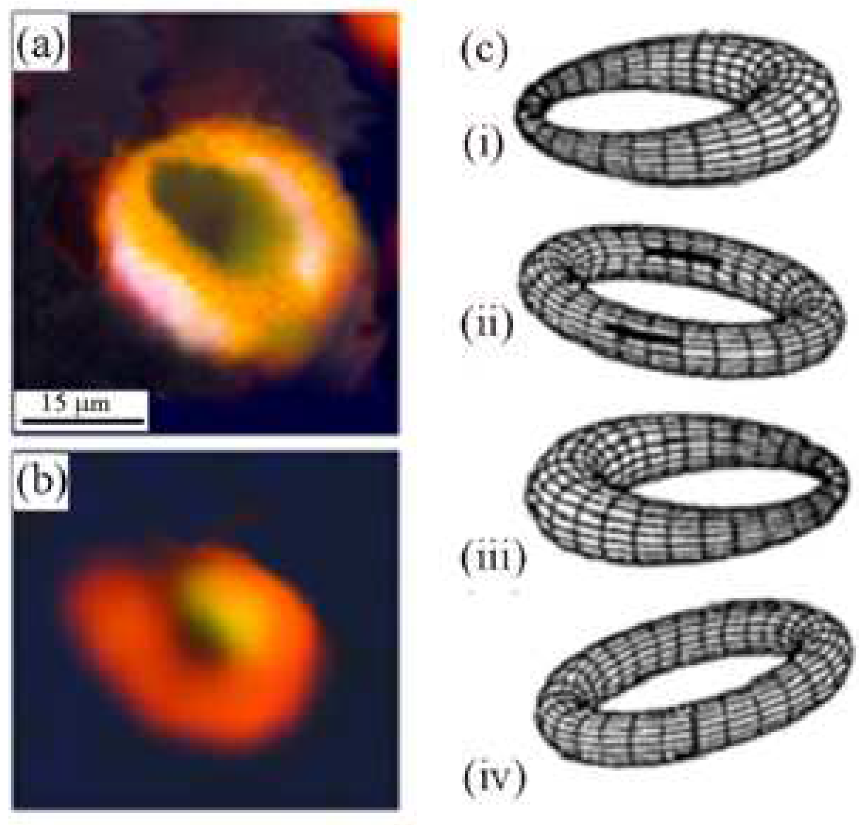
Vortex rings generated by the breakdown of loops under the action of cut-and-connect operation may be assumed—circular cylindrical vortices with a Gaussian vorticity (known as the Oseen vortices). Under local random multipolar strains in the laser spot, these vortices show the evolution of various types of instabilities. Comparison with theoretical results enabled hierarchical classification of these instabilities. It was shown that the velocity field of an unstable wave on Kelvin’s vortex ring (that is, constant vorticity at leading order) can be expressed in terms of the Bessel and modified Bessel functions [69,70,71]. The order of Bessel functions introduces azimuthal length scale, axial wavenumber, and axial length scale, as well as radial wavenumber for nodal structures of the core. They originate from parametric resonance instability caused by the effect of toroidal curvature [68,69,70,71,72,73] and are called Widnall–Bliss–Tsai (WBT) instability [74].

An important finding of this study—consistent with our previous results [58]—is that among many structures, four types of vortex ring instability modes can be identified in laser interactions as the basic structures; two of them (I)—left- and right-handed helical waves and (II)—curvature instability are parametric resonances, while III and IV are the long wavelength oscillations.

Type I of the vortex ring instability obtained by LMI s is based on “WBT instability”, which originates from the elliptical core deformation and includes parametric resonance of the left- and right-handed helical waves (m = ±1). This type includes also helical–helical wave resonance (m, m + 2) = (−1, 1), which consists of the left-and right-handed quasi-stationary helical waves.

This instability on the vortex rings of the diameter 2R~28–30 μm (comparable with the radius 2R~26 μm in ref. [58]) is given in Figure 9.

Type II of the vortex ring instability is also based on WBT instability and identified as the “curvature instability”, which includes parametric resonance between the helical (m = 1) and the bulge (m = 0) modes [58]. Vortex ring instability of the helical–bulge wave resonance (m, m + 1) = (0,1) is shown in Figure 10.

Type III of vortex ring instability is identified as the Kelvin axisymmetric mode or the “bulge wave” (m = 0) [58]. The “bulge wave” for which the S1-symmetry of the circular core is created by the combination of the axisymmetric (m = 0) and the bending (m = 1) waves (Figure 11).

Figure 11a shows the initial stage of instability while Figure 11b shows the final stage after the breakup of the ring when the oscillation reaches the critical level. The schematic illustration in Figure 11c(i–iv) shows a standing deformation mode of the core cross-section shown in Figure 10 of Kop’ev and Chernyshev in Ref. [75].

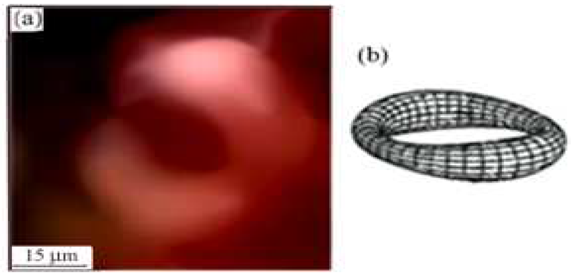
Type IV of the vortex ring instability is identified as the “standing deformation mode”, created by the long wavelength oscillations of multiple Kelvin waves combined of m = 0 and m = ±1 modes, shown in Figure 12a and schematic illustration, and Figure 12b of Kop’ev and Chernyshev [75].

The findings of four types of vortex ring instabilities indicate that they are caused by nonselective, spatially inhomogeneous shock-induced excitation—in the regions of the low filament density (Λ > σ). Under conditions dominating in these regions, a vortex ring can accommodate a number of instability modes creating the structures related to a parametric resonance instability caused by dipolar and quadrupolar fields. This gives a clearly better understanding of the shock wave effects, which create vorticity, but also may alter the picture established by a theory of homogeneous media.

4.1.5. Vortex Filament “Complexes”

Besides the above findings, characteristic of the regions of a low filament density, our experiments also demonstrate that multipulse laser interaction (with a Co-coated steel target) creates very complex patterns—in the regions of a high vortex filament density (Λ ~ σ). Vortex filament dynamics leading to such structures are caused by inhomogeneous turbulence and various strain fields in the fluid layer. Under the action of strain fields, vortex filaments form coils, helices, bundles, and other structures, which we refer to as “complexes” [61] The strain fields can be (quasi-)static or oscillatory, creating torsional and twisting filamentary structures ranging from the nanometer to the millimeter scale. With increasing N, filaments become collected into axially merged bundles, merged into thick filaments, or transformed into ribbons and tubular ribbons. Their interaction with localized strain fields gives rise to various types of complex structures with complexity being controlled by the number of pulses and the density of the vortex filament array [61].

4.2. Formation of Vortex Filament “Complexes”

A series of laser pulses causes the motion of vortex filaments and collective behavior with the formation of vortex filament bundles, helically paired structures, and the formation of multiple loop solitons on bundles. While the first pulses cause the roll-up of the shear layer into vortex filaments (for Re > Re_critical; Re_critical~10⁴), and the formation of a parallel array, the other pulses cause their motion. Strong transversal oscillation and motion of filaments cause their aggregation in the regions of the minimum strain [61]. If lateral (parallel to the surface) and vertical (normal) strain field components are comparable, the filaments move closer and form a bundle. Immersed in the turbulent background fluid, vortex filament bundles also experience the oscillatory strain field of background fluid, which causes twisting and winding, helical pairing, formation of double helices of bundles, braiding, and tangling, and formation of loops on the bundles as well, giving rise to the above-mentioned complex structures, which we refer to as “complexes” [61].

Such filament–bundle “complex”, which forms a double helix shown in Figure 13a, (and in the refined micrograph in Figure 13b), is obtained for the first time.

Schematic reconstruction of vortex filaments organized into bundles, which form a double helix in Figure 13, is shown in three consecutive steps, starting with two bundles of parallel vortex filaments, which are exposed to torsion, is shown in Figure 14.

While many filaments are firmly incorporated into bundles, some of them (slightly separated from the mother bundle) show individual behavior with the formation of the loop solitons—thus giving rise to the filament-bundle “complex”.

Extensive results carried out also show the formation of even more complex bundle structures in multipulse LMI. Figure 15 shows that vortex filament bundles exposed to torsion and twist-perturbation cause the successive formation of (+) and (−) soliton loops, as well as the filament coiling—which we obtained for the first time.

This picture (left side) also shows two connected rings, which are formed after loop soliton breakup, meaning that they are formed by the “cut and connect” operation. Once formed, the rings stay in the vicinity of the mother filament, but the strong core diffusion makes the surrounding ambient in a turbulent background field, rather misty. An approximate reconstruction of this “complex” is given in Figure 16a.

Schematic illustration of the interaction of (+) and (−) loop solitons (i) leads to their annihilation (ii) as shown in Figure 16b. With subsequent laser pulses, a bundle of vortex filaments is exposed to growing compression, which invites resistance to the filament motion and causes the axial to merge into a thick vortex filament [61]. In that case, the formation of a vortex filament bundle consisting of thick and thin filaments (under an oscillating pressure field) is associated with the motion of the peripheral filaments, which become slightly shifted from thick filaments. Under torsion, the helical motion of thick and thin filaments creates “complex” with (+) and (−) loop solitons (Figure 17).

Under a series of pulses, thick and thin filaments may show individual translative motion and wiggling; however, a thin filament mostly follows the curvature of a thick one. In the inhomogeneous flow field of the laser spot, such vortex filaments experience different torsion, stretching, etc. Therefore, the loop solitons of different radii and curvature will be formed making a highly complex structure. In the oscillatory strain field of laser shocks, vortex filaments may also form a series of kinks and, if they come into close vicinity, may axially merge or form chaotic structures depending on the number N of laser pulses. When N reaches the critical level, N = N_crit, the loop-soliton breakup will form open loops, which may become connected to vortex rings [61].

An important finding in the understanding of this phenomenon is that the process starts with one filament approaching its neighbor; the approaching filament longitudinally stretches while its cross-section narrows. As the angular momentum is conserved, the vortex filament spins faster enhancing the co-rotation of the same signed filamentary vortices, intensifying viscous diffusion. The crucial role in axial merging—and the formation of thick vortex filament—is played by the viscous diffusion term, a source term due to stretching, but also an advection term with variable advection speed [61]. Intense laser pulses of ~10⁸ W/cm², create plasma—which together with molten target surface—establishes the layer of low- and high-density fluids, separated by the density interface. The shock-induced acceleration of density interface and variable density flow lead to the RM/RT instability and the formation of vortex-filament structures like bundles and their “complexes”. Since very little is known about the filament-bundle “complexes”—the above results provide evidence on their formation and behavior in the oscillatory shock-induced environment.

The mechanisms responsible for their formation and behavior operate in and between many different scales. Along this line of thinking, the nonlinear and nonequilibrium processes that lead to the formation of the small-scale structures created by laser experiments on metal targets at medium power density are mimic of those characteristic for the large-scale near-peripheral region of the Crab Nebula.

5. Basic Aspects of Astrophysical Plasma Systems: Nebulas

Astrophysical plasma systems like Cosmic nebulas are generated by various mechanisms and appear in various shapes and sizes, which extend over many light years. Some nebulas are formed from interstellar gas (dust particles and molecular species), which under twisting magnetic lines creates helicoidal filamentary structures—such as Double-Helix Nebula. The other nebulas created by the collapse of stars represent the remnants of supernovae—actually, a thin plasmatic shock area at its boundary exposed to magnetic fields, which affect the behavior of expanding matter [1]. A spherical blast wave propagates from the center of a star outwards through the star’s layers of gradually less-dense gases, causing the shock-induced variable density flow thus generating the RT instability [1,76] and wave–vortex structures. This shock wave expands into the surrounding interstellar medium, sweeping up an expanding shell of gas and dust. The ejected debris mixes with the interstellar medium and forms a nebulas a supernova remnant [76,77], such as the Crab Nebula.

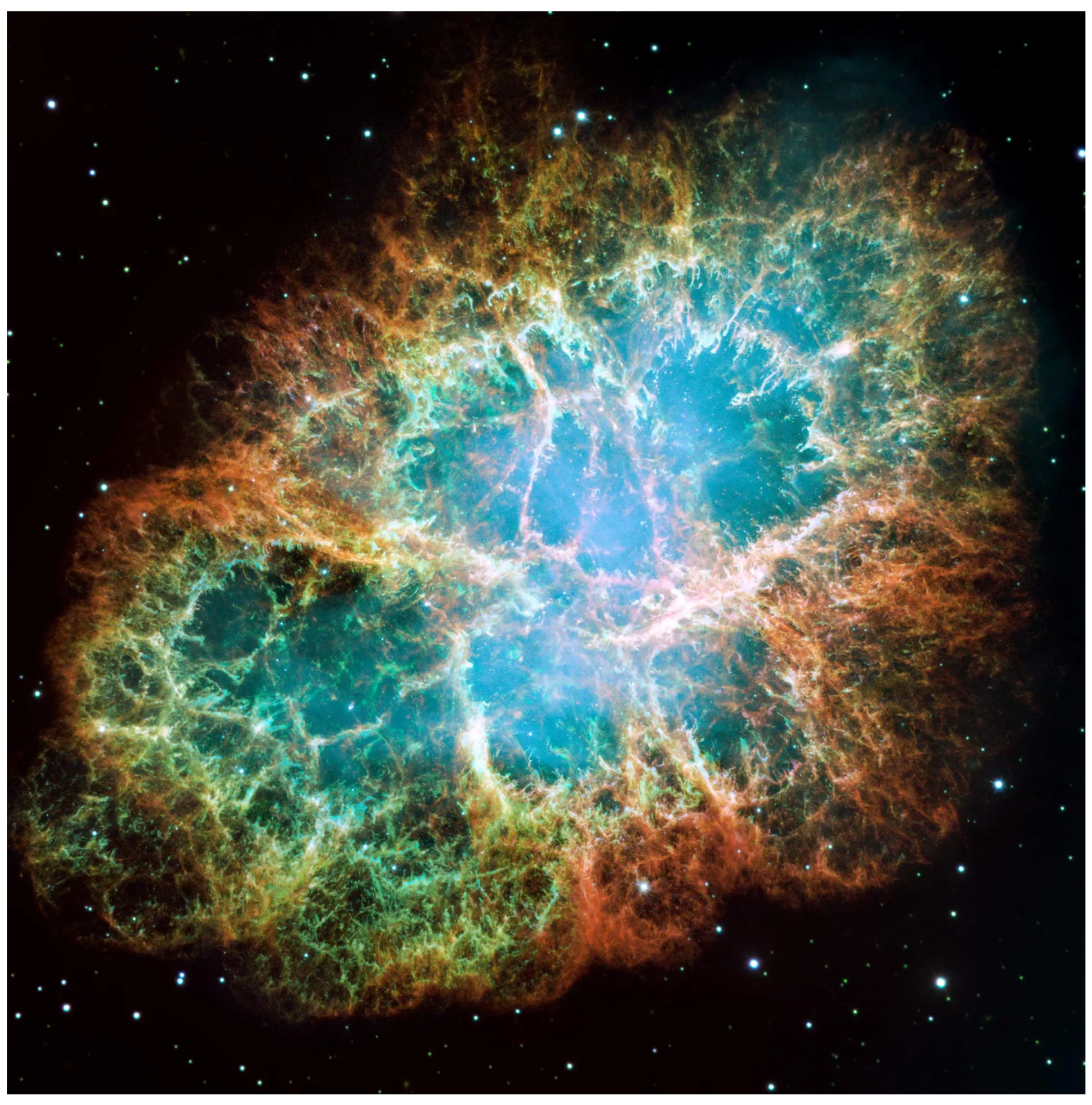
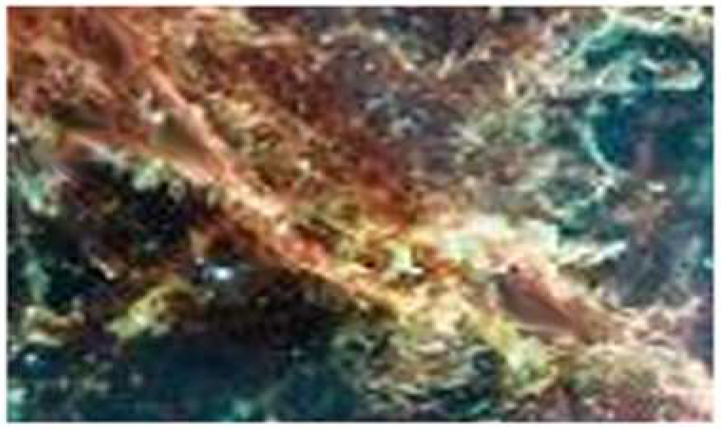
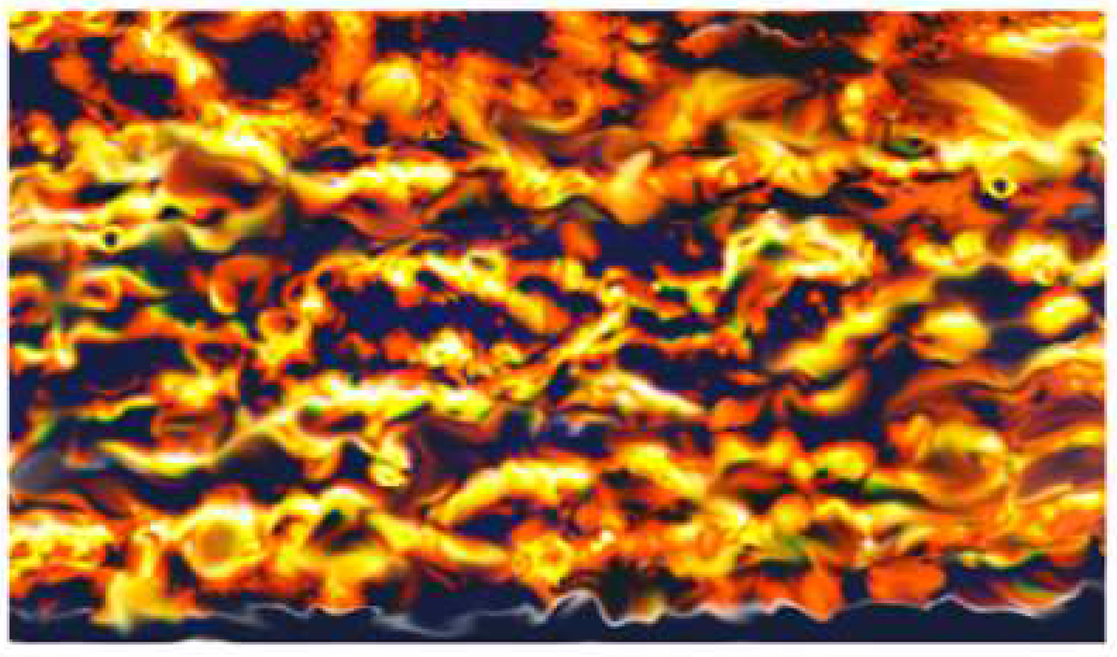
The picture of the Crab Nebula (Figure 18) reveals its composition and structure [78] and provides a starting point for the study of regular and irregular structures and cluster formations.

The diffuse blue region of Crab Nebula is generated by the synchrotron radiation caused by electrons moving at relativistic speeds [79] along trajectories curved by the strong magnetic field, which originates from a spinning neutron star—a pulsar (the ultra-dense core of the exploded star)—at the center of the Nebula [80]. Electrons circulating around the magnetic field lines create this blue light in the interior of the synchrotron nebula, which is bounded by the thermal ejecta. Both the synchrotron nebula and filament structures are embedded in the expanding supernova plasmatic remnant. According to Hester [81], these structures—called thermal filaments—are composed of ejecta from the explosion and located around the outer part of the synchrotron nebula. The ejecta evolving along the magnetic field lines take the form of vortex filaments, filament jets, knotted filaments, loops, etc., which are dominated by the line emission [79,82] They consist of ionized helium and hydrogen, as well as carbon, oxygen, nitrogen, iron, neon, and sulfur, which create colored structures [82] (Figure 18). Spectroscopic diagnostics reveal that orange filaments consist mostly of hydrogen, while green ones consist of singly ionized sulfur. In the outer part of the nebula, dominating blue filaments originate from neutral oxygen, while red ones originate from doubly ionized oxygen [78]. This highly ionized red region makes a “skin” around the synchrotron emission. This red “skin” is driven into a larger, expanding remnant, which surrounds the crab. Within this expanding remnant, there are dense structures of “thermal filaments” with self-shielded cores that are highly ionized [59]. Spectroscopy of multiply ionized Oxygen III reveals that temperatures of thermal filaments range from ~12,000 K to 20,000 K [59]. Somewhat different values are obtained from other measurements, which give the filaments’ temperatures about ~11,000–18,000 K, and their densities about ~1300 particles per cm³ [63] Morphological properties of these particle structures in the Crab Nebula are described in [83].

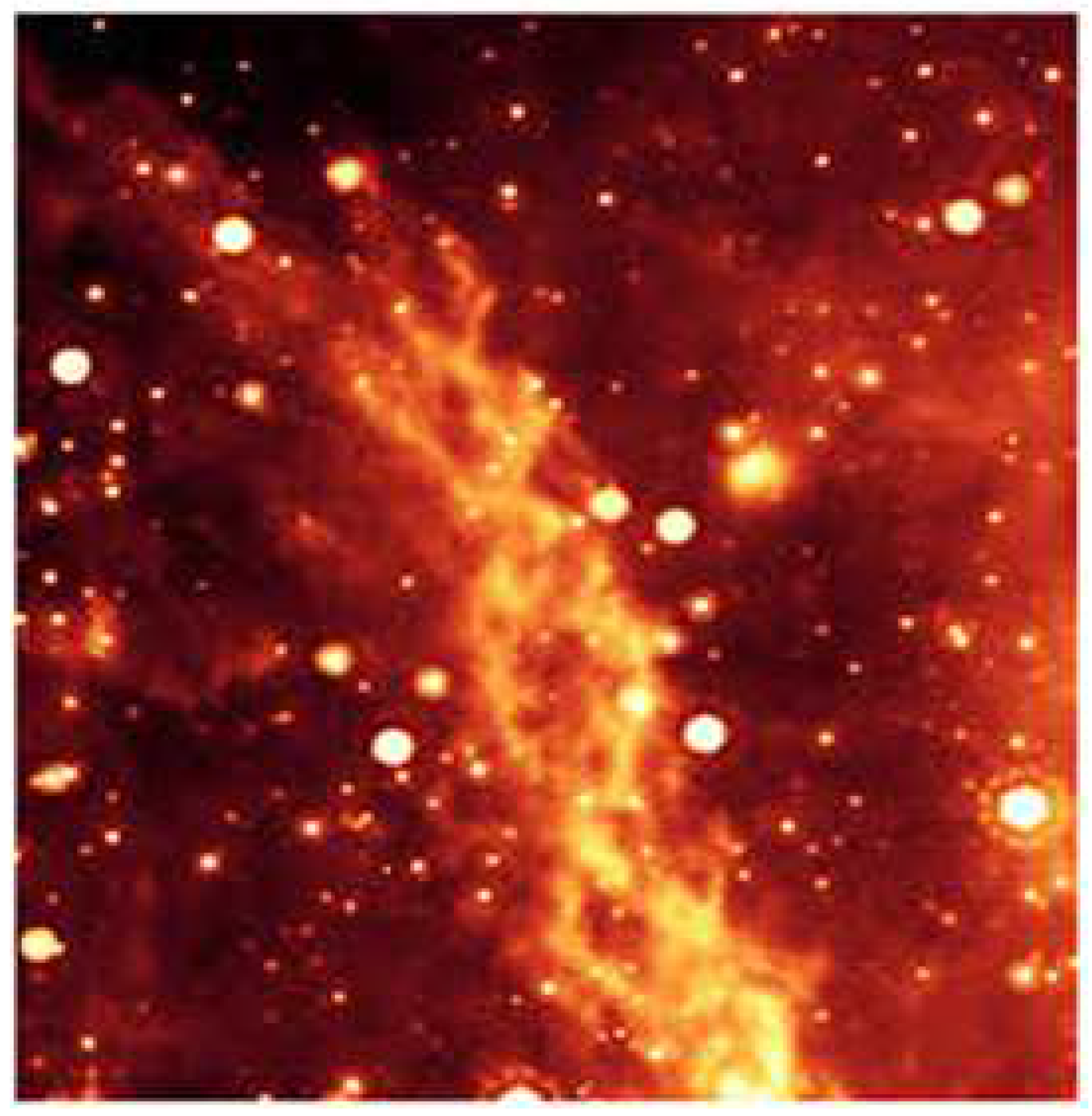
Particles and the wind of waves streaming in a radial direction are emitted from the pulsar in the central part of the nebula, which loses its rotational energy emitting a relativistic wind of waves and particles. They interact with the surrounding ambient, generating pulsar wind nebulae (PWNe), observable from radio to γ-rays. PWNe often shows a torus–jet structure [84]. Orientation of the torus–jet structures is referenced with respect to the line of sight to the Earth: For the view of the front side of the remnant, the north is up and the east is to the left. The other view 60° E from the line of sight to the Earth, and 30° S of the E–W plane gives a different picture. This is roughly equivalent to viewing the remnant from the southeast, sighting along the major optical axis. All jets and filament structures are arranged in a pattern that can best be described in relation to the plane of the E–W torus [85]. In this respect, the most impressive magnetized jet is the “South-East (SE) jet” of the Crab Nebula, which was recently studied in scaled experiments by ultraintense laser [5].

Regarding the interaction of ejected plasma particles with the surrounding medium, the study of Kuranzet al. [86] reveals that various unstable processes in the nebula create convoluted structures at boundaries between regions, with significant interpenetration of the plasmatic matter from one region to the next. This is evident in the regions where spikes of high-density stellar ejecta penetrate into the PWN [86], initiating the Rayleigh–Taylor instability and mixing. Rayleigh–Taylor instability leads to intense mixing, the characteristics of which depend on the local velocity, scale of structure growth, and the scale of energy dissipation, which determine the width of the mixing zone—mostly different in different regions of the huge plasmatic system. In addition, there are suggestions that some other processes may also play a role in the material mixing scenario—besides RT and RM instabilities [87].

The velocity of the plasma jet at the Crab Nebula periphery is ~100 km/s with respect to the nebular expansion velocity [88]. Based on the radio image, the equilibrium magnetic field of the “jet” appears well ordered, while the density of the thermal gas inside the plasma jet is estimated to be ~0.7/cm³, and the Alfven velocity is more than ~700 km/s. It is suggested that “The “jet” is probably confined most likely by a toroidal magnetic field which must be of the same order of magnitude, i.e., 3 × 10⁻⁴ G, resulting in a helical field” [88] For comparison, in solar flares, the magnetic fields are of the order of hundreds of Gauss with a maximum of ~10–50 G [89]. Also, the plasma density in solar flares is of the order of 10⁹ to 10¹⁰ cm⁻³ [89], while in the central part of the nebula (pulsar wind nebulas), the ambient number density is only ~0.1 cm⁻³ [90,91].

The surface magnetic dipole of radio pulsars has a strength of B~10¹¹⁻¹³ G [92],which for the Crab Nebula is estimated to be ~7.6 × 10¹² G [93] , while in its peripheral region the strength is ~300–500 μG [94]. The strength of the magnetic field is the parameter, which—in combination with velocity and plasma particle density—dictates the dynamics, morphological, and topological characteristics of ejecta. The ejecta take the form of long magnetized jets in the near central region of the strong magnetic field, and the form of filaments, filament loops, etc., in the near peripheral region of the weak magnetic field, in the Crab Nebula. These plasmatic structures in the nebula can be analyzed relaying on the analogy with similar structures evolving from nonlinear and nonequilibrium processes at the microscale created by intense and ultraintense lasers.

6. Crab Nebula: Filament “Complexes” in the near Periphery Region

Crab Nebula (Figure 18) consists of (i) an external supernova remnant (SNR) as a diffuse, expanding nebula plasma shell, and (ii) an inner pulsar wind nebula (PWN) inside the shell of a supernova remnant (SNR), driven by winds from the central pulsar.

6.1. Magnetized Vortex Filaments and Loop Solitons in the Peripheral Region of the Crab Nebula: Weak Magnetic Field

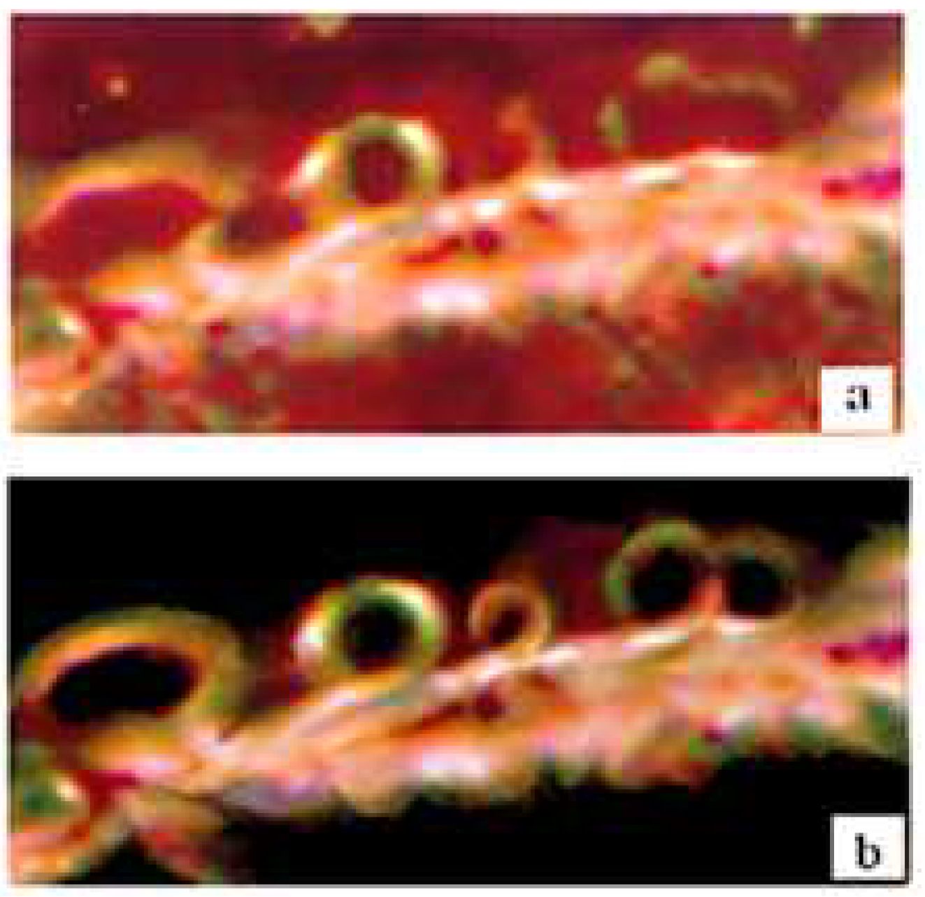
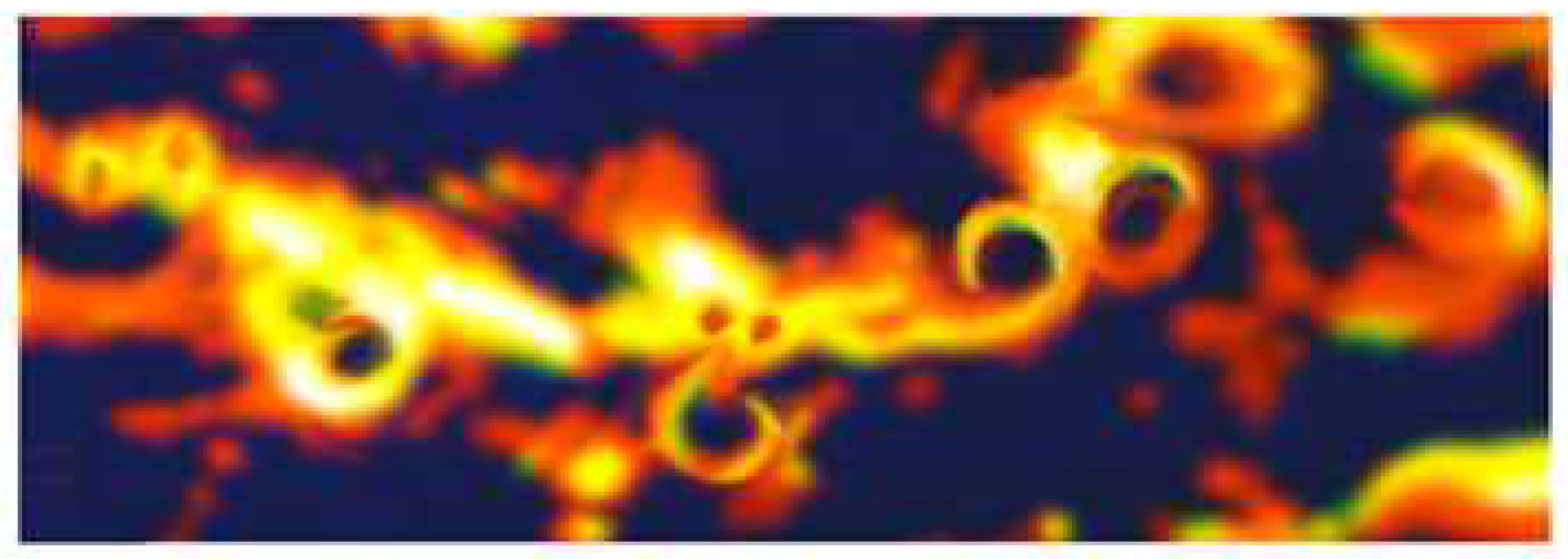
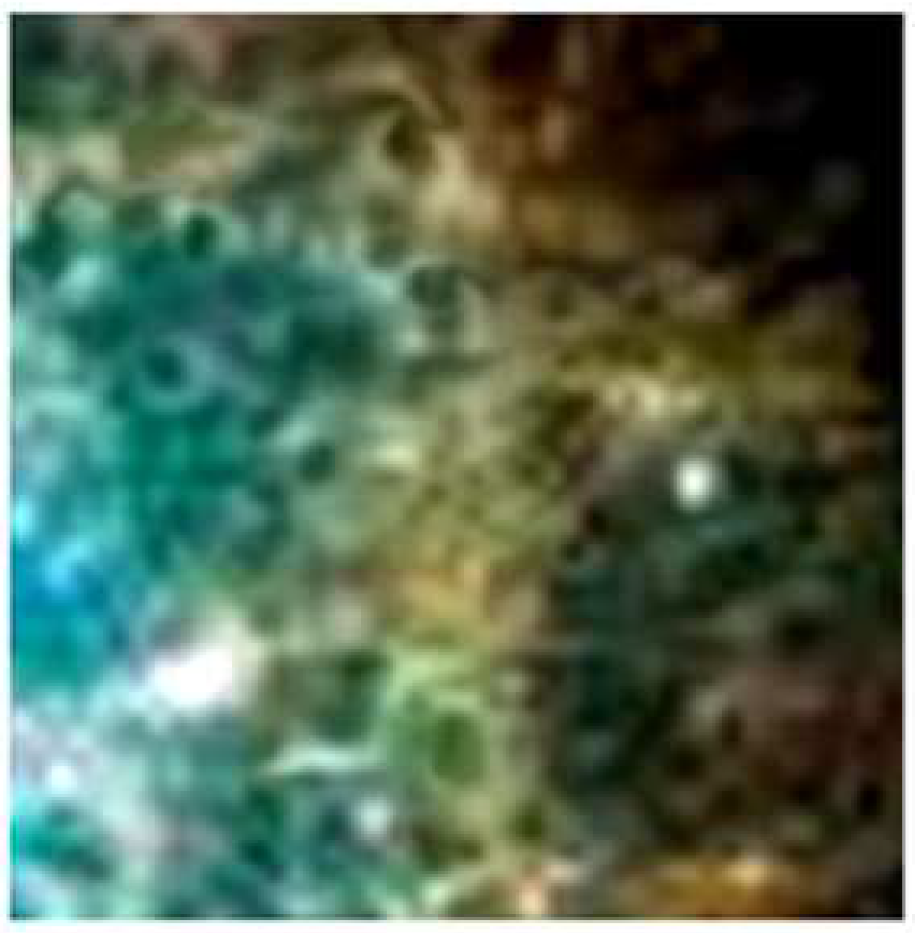
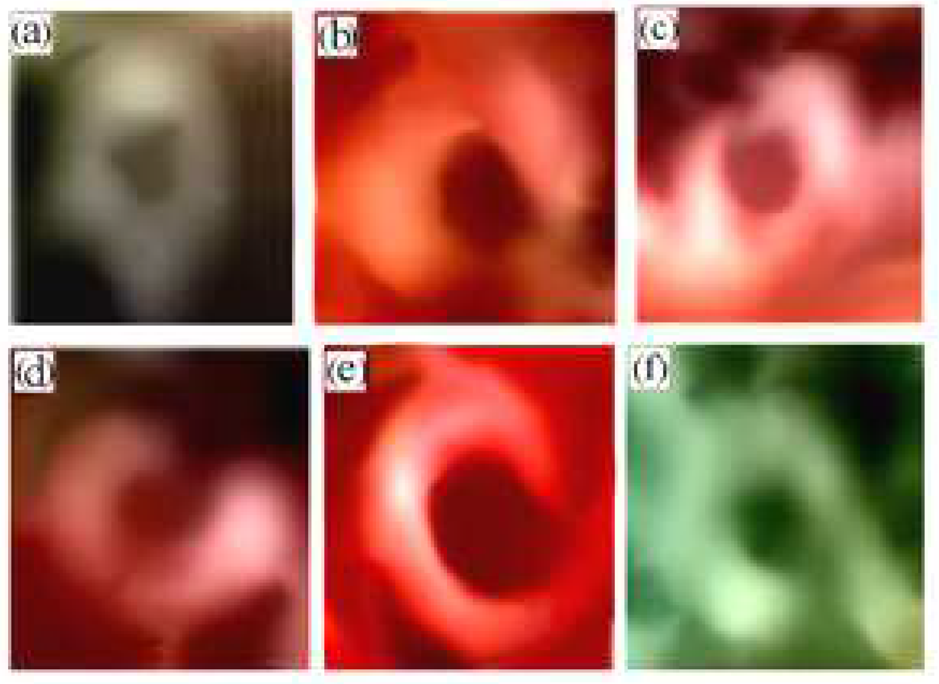
A diffuse supernova remnant of expanding nebula shell at the external side of the PWN/SNR boundary, where the magnetic field is weak, represents the peripheral and the near peripheral region of the Crab Nebula. A large magnification (besides filaments) also shows filament loop solitons, vortex rings, and broken rings (Figure 19).

These loop solitons (created by winding of particle trajectories along the magnetic field lines) are similar to those in LMI (created by winding of vortex filaments by mechanical torsional strain). A number of random loop solitons in the right peripheral crab region can also be seen in Figure 19. These loop solitons appear in different colors in two different parts of this region, characteristic of different plasma compositions of ionized gases. They are mostly closed loops, indicating equal (constant) plasma acceleration (equal magnetic field strength and winding), meaning that the instability of these filaments did not reach the critical level for their breakup.

Very similar loop soliton structures can be seen in other peripheral regions of the Crab Nebula. An example is the upper peripheral left region. The loop solitons also appear in two different colors, but in contrast to the right region, the loops are mostly broken (in the green part), while some of the loops are closed or even appear as rings (in the brown part) of this region. This indicates spatially variable plasma acceleration (or variable magnetic field strength), meaning that the instability of filaments reached the critical level for their breakup in the green part, and did not reach it in the brown part of the region. This may indicate the inhomogeneity of the plasmatic and magnetic field(Figure 20).

Conjecture may be established with the multipulse LMI, where the loop solitons on vortex filaments reach the instability threshold after a critical number of pulses and spatially variable acceleration—becoming broken into open loops and later on into vortex rings. Common to both cases is the underlying helical motion of the vortex filament (in LMI) and of the magnetized filament (in nebula), which is characteristic of many astrophysical systems. In this respect, the formation of the loop solitons on magnetized vortex filaments in the Crab Nebula—as the nonlinear and nonequilibrium phenomenon—is analogous to the formation of the knot solitons [95] to the visible hot spot soliton-like points on magnetized jets and to the solitons caused by torsion of the magnetic field lines (filament jets) in “magnetars”—the magnetic stars [96,97,98]. Considering magnetized knotted jets in active galactic nuclei (radio galaxy 3C303), Lapenta and Kronberg [95] defined knots as “visual manifestation of an underlying helical form of a jet, which can also be explained as shocks along the jets that heat the plasma particles, creating visible hot spot”. The other interpretations are based on “the Kelvin–Helmholtz instability, and on current-driven modes, but also on the model which considers the jets with knotted solitary structure as actual plasma features, which are ejected from the accretion disc and propagate along the jet axis” [95]. Based on this approach, Lapenta [95] used a mathematical analogy between the stationary magnetohydrodynamic (MHD) equations (Grad–Shafranov equation) and the nonlinear Schrodinger equation for soliton propagation. Taking the magnetized jet that propagates along the z-direction perpendicular to the (x,y) plane, and neglecting the y-direction, the problem is reduced to 2D solutions in the (x,z) plane, with the system size Lx and Lz [95]. The solution is constructed as a mathematical analogy to the soliton equation for nonlinear wave propagation (cubic Schrodinger equation). The magnetic field is obtained from a flux function as described by Lapenta and Kromberg [95].

$$\Psi ={\mathit{\Psi }}_p\sec h(x/L)e^{ikz}$$

(20)

where ᴪ_p is the on-plane magnetic field. This equation for the magnetized jet with knotty structure is just the same equation of Hasimoto transformation (11) for the loop soliton on vortex filament in LMI (where ᴪ_p corresponds to torsion) [95], which makes an analogy between similar instabilities at the micro- and megascale.

The system evolution has two phases: a long period of stability followed by sudden instability. The stable phase corresponds to the long collimation phase of the magnetized filament jet, appearing as a straight regular structure. The knots characterize the periodic “bubbly” structure of the solitons. Such soliton-like solutions reveal that a magnetic field amplitude grows through periodic alternating minima and maxima. This feature is common to the well-known coherence of solitons in many areas of physics, in which nonlinear equations admit soliton solutions [95].

The origin of loop-soliton-like structures was also studied as the result of the torsion of magnetic vortex line curves [96]. According to Ricca [97], torsion in twisted vortex filaments affects significantly the motion of helical vortex filaments, in the fluid, where the binormal component is responsible for the displacement of the vortex filament. Based on this approach, Andarde [96] solved the equilibrium equations of magnetic stars for vortex filaments and wrote the magnetar equations in the Frenet–Serret frame for constant torsion. It was shown that the magnetic field oscillates in a helical form, and the behavior of magnetized vortex filament follows the Hasimoto transformation of the Schrodinger equation for the constant torsion creating loop solitary structures. Long vortex filaments and underlying helical motion due to magnetic torsional strain field(s) lead to the formation of the series of loop solitons, which are quite similar to the string of the loop solitons on vortex filaments in LMI. The creation of multisolitons of different radii and curvature, which travel at different velocities, and their nonlinear interaction may cause their complex organization in space. A complex case occurs when two solitons of the same polarity of the wavevector (either + or −) collide from behind, and a more complex case occurs when they have different polarity [66].

Such a loop-soliton chain on magnetized filamentary jets in the peripheral crab region is shown in Figure 21.

6.2. Vortex Ring Instabilities in the Near Peripheral Region of the Crab Nebula

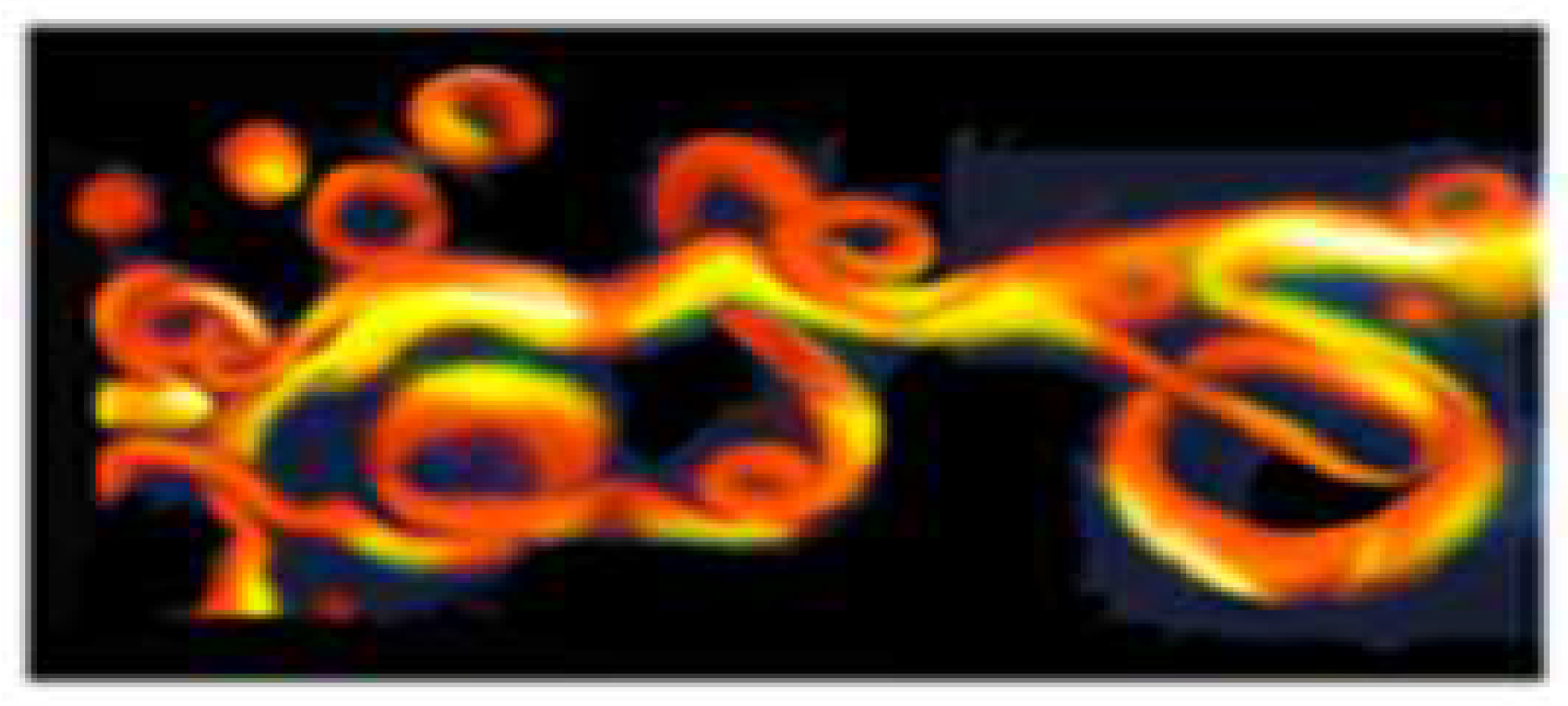
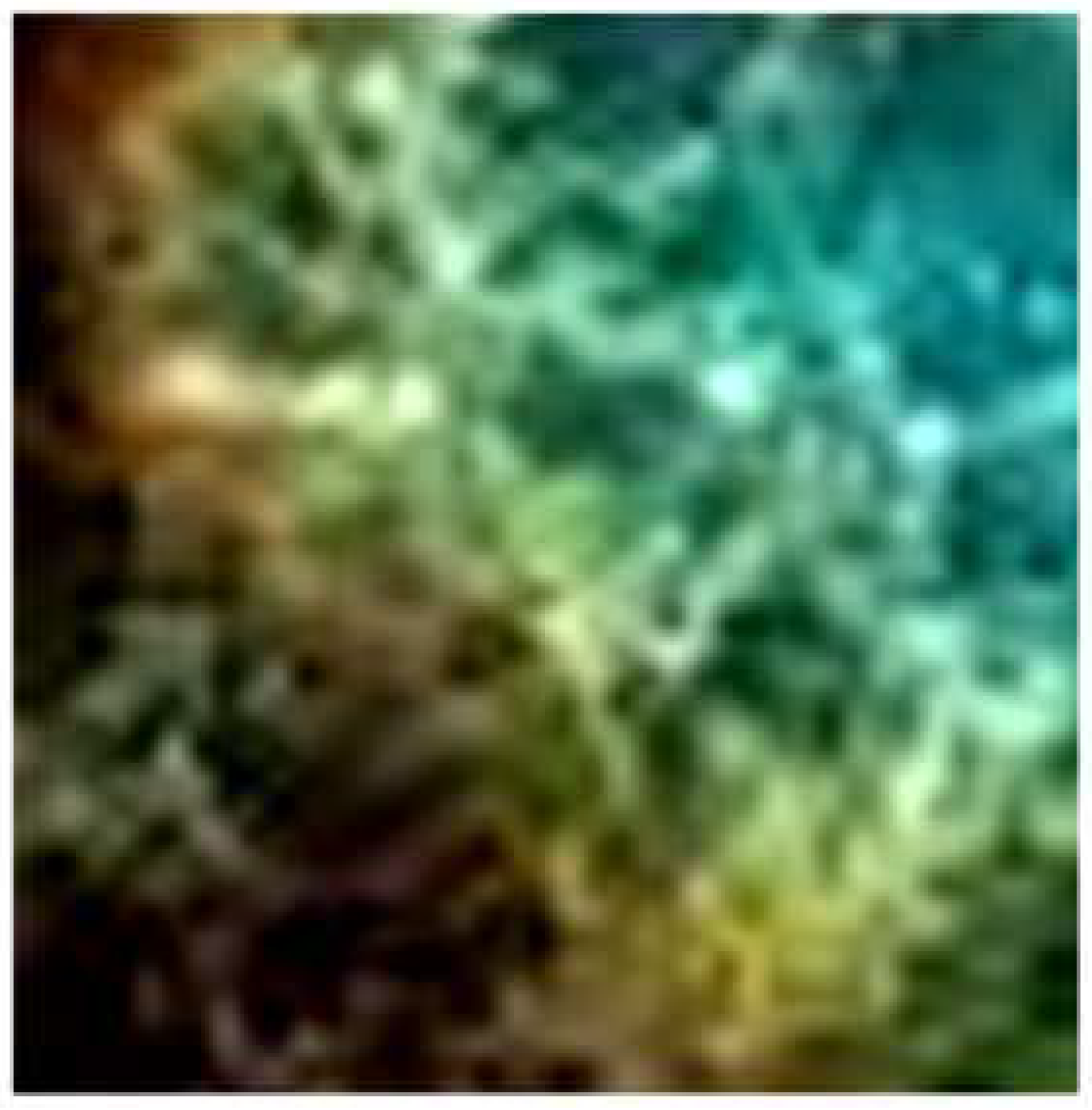
Peripheral regions of the Crab Nebula under magnification also reveal deformed and broken rings as well as the open loops in the vicinity of the string of the loop solitons on filaments (Figure 22).

Morphological and topological characteristics of broken loops, rings, and deformed vortex rings of the Crab Nebula indicate that these ring instabilities may eventually be attributed to the same classification as those generated in the multipulse LMI, shown in Figure 10, Figure 11, Figure 12 and Figure 13.

Based on this classification, characteristics of the shape, symmetry, and oscillation modes of broken rings and open loops of the crab in Figure 22 indicate the ring axisymmetric instability of type III, called the bulge wave. This instability still has circular symmetry and corresponds to the case of the vortex axis tilted [58]. However, broken rings indicate that this instability has reached a critical level for the integrity of the rings.

6.3. Evolution of Rayleigh–Taylor Instability at the PWN/SNR Boundary of the Crab Nebula

A diffuse supernova remnant of an expanding nebula shell at the PWN/SNR boundary experiences the pulsar wind from the central region, which expands radially driving a hot plasmatic bubble (PWN-bubble) into a colder external SNR shell. The high pressure of the hot PWN bubble drives a shock wave into the high-density cold ejecta causing the formation of a density interface [99,100]. The interface perturbation evolves into Rayleigh–Taylor (RT) instability with the growth of spike fingers oriented downwards and bubbles growing between the fingers (RTI spikes). According to [101,102], the RTI is the origin of the “thermal filaments” observed in the near peripheral regions of the Crab Nebula—the outer side of the PWN/SNR boundary.

At the contact discontinuity between PWN and SNR regions of the Crab Nebula, these RTI structures dominate. Using the self-similar model of PWN inflating the ejecta with density ρ ∝r^−α by a pulsar wind, it was found that the shock speed that causes growth of RTI can be expressed [103,104] as follows:

$$V_{shock}=t^{1/(5-\alpha )}$$

(21)

where α is the index of the jet ejecta density distribution; for uniform ejecta α = 0. Starting with the linear regime, the RTI growth switches into the non-linear regime when the amplitude of the interface distortion becomes comparable to the wavelength λ. At the onset of this regime, the light fluid creates bubbles/columns of diameter ~λ, which steadily rise with the speed:

$$v_{bubble}\approx 0.5\sqrt{g\lambda }$$

(22)

while the heavy fluid forms thin fingers in the Crab Nebula approaching the free-fall regime, as observed by a number of authors between 1950 and 2012 (listed by Porth et al. [85] and later shown by more complex 3D simulations.

Regarding the location (regions) of their appearance, there are statements like “Most individual filaments are small-scale structures but some are much longer and appear to cross almost the entire nebula”, but also “the filaments with low line-of-sight speed avoid the central region of the nebula image” [85]. This indicates that the crab filaments do not penetrate the whole volume of the nebula, as otherwise low line-of-sight speed emission would be seen there. Instead, “the filaments reside near its outer edge, where they occupy a thick shell of thickness about one-third of the nebula radius” [85,104], which is of the size ~1.83 ly. In addition, some authors when describing tiny filamentary structures refer to them as “threads”—a characteristic of the near central region (the PWN dominant region)—and not for the shell region.

Numerical simulations reveal that the evolution of RTI at the contact discontinuity between PWN and SNR regions creates coherent filamentary structures. These simulated coherent RT finger-spike structures or filaments resemble some of the real crab filaments; the longest ones reach the length of ~1/4 of the nebula radius (r = 5.5 ly). Regarding the formation of such long filaments, the picture is not quite clear. Namely, as mentioned by Porth et al. [105], the thickness of the mixing layer occupied by the RTI fingers is much smaller, only approximately 1/15 of the PWN radius—which is about five times below the thickness of the Crab’s filamentary shell.

However, in spite of some uncertainness, the point to be emphasized is that filaments are identified as the “Rayleigh–Taylor filaments” (actually tiny RTI spikes), resulting from the nonlinear evolution in the presence of the magnetic field. Hester et al. [94] applied the theory of magnetic RTI, assuming that the smallest structures of the Crab’s filamentary network resemble the RT bubbles and fingers with the wavelength of λ = 2λ_c, for ρ₂ >> ρ₁. Simulations have shown different effects on the RT modes with respect to the direction of the magnetic field.

For the RT modes normal to the magnetic field, the growth rate of the non-magnetic case is recovered—the magnetic field does not suppress modes normal to the magnetic field.

For RT modes parallel to the field, the magnetic tension suppresses the perturbations with wavelengths below the critical one, λ_c (full suppression).

The presence of a magnetic field is expected to have a significant effect because pulsar winds inject highly magnetized plasma into the PWN bubble. Such a strong magnetic field should suppress the evolution of RTI and of the filamentary structures. However, “the 3D simulations have shown that because of the strong magnetic dissipation and field randomization—the magnetic tension at the contact discontinuity between PWN and SNR regions is not strong enough to suppress the growth of RT filaments”, so that prominent filaments appear in the Crab Nebula [103].

7. The Crab Nebula near Central Region: Formation of Filament “Complexes”

7.1. Bundles of Filaments Helically Paired: Very Strong Magnetic Field

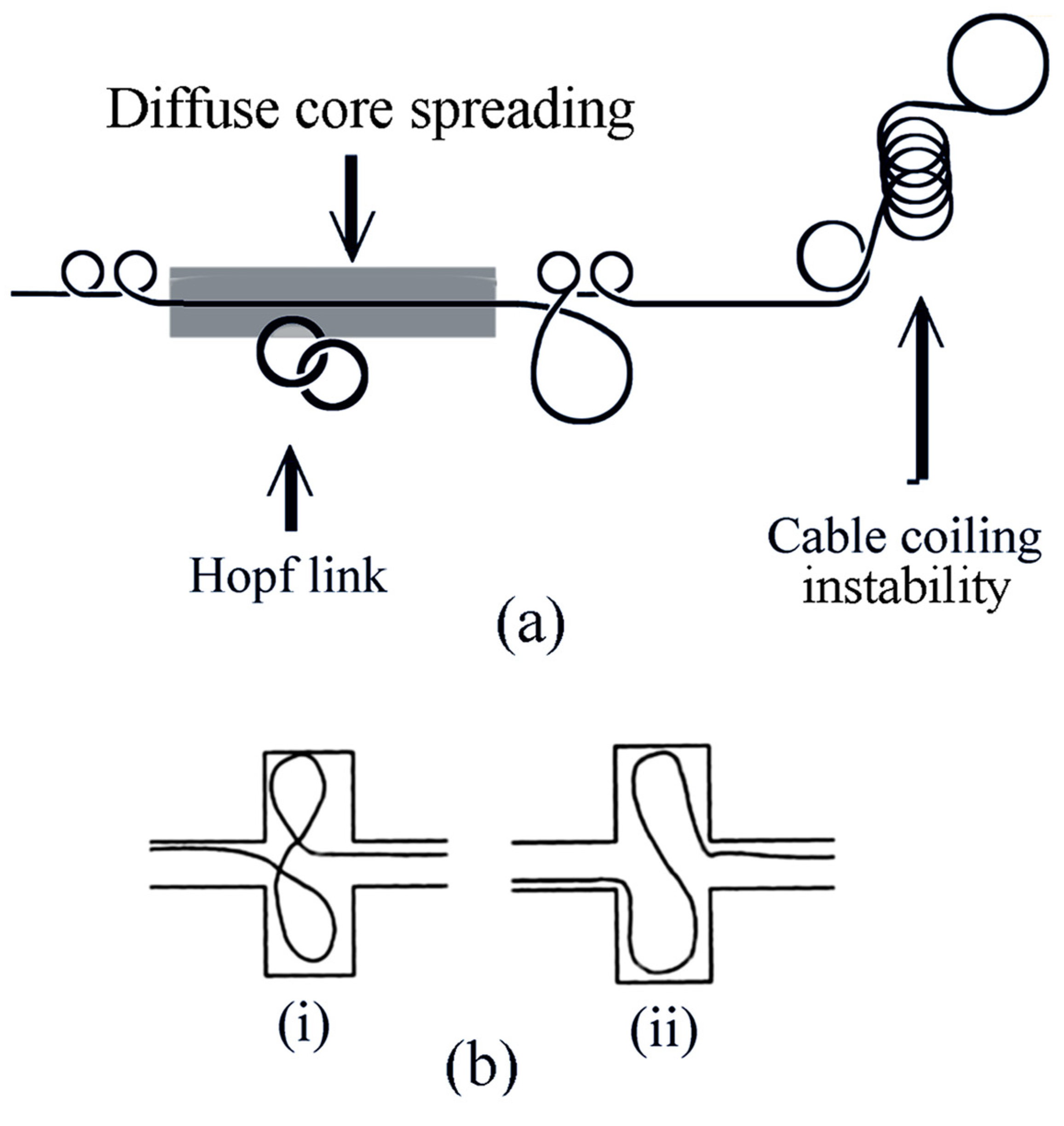
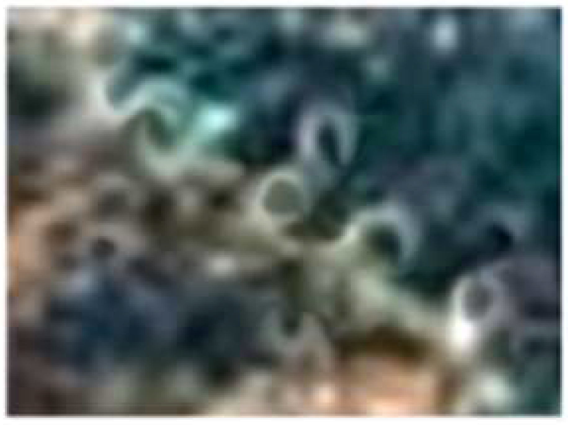
Inside the shell of a supernova remnant (SNR)—in the near central region of the Crab Nebula—different phenomena dominate driven by winds from a central pulsar (PWN), where the magnetic field is very strong. A strong magnetic field overwhelms the plasma shear flow instability, suppresses the RTI evolution, and has a dominant role in the formation of magnetized filament jets [105]. Magnification of this region of the Crab Nebula reveals long filament jets organized into bundles, which form double helices—a kind of “complexes” (Figure 23 and Figure 24).

Double helices—a kind of “complexes on bundles”—are caused by twisting of magnetized bundles of filament jets. Magnification of two segments of the double helix in Figure 24a,b reveals vortex rings and loops on those magnetized filaments, which are slightly separated from bundles and manifest individual behavior. These loop solitons, as well as vortex rings and broken rings in the near central region of the Crab Nebula, are quite similar to those observed on vortex filament bundles created by multipulse LMI.

Another type of magnetized filament “bundles” that form a double helix (selected from the upper central part of the Crab Nebula in Figure 18) is shown in Figure 25.

The double helix consists of fragmented magnetized filaments, which connects the blue central part and the brown-yellow peripheral part in the Crab Nebula. In contrast to bundles of the long filament jets in Figure 23 and Figure 24, these “bundles” are composed of fine filaments (like threads) much shorter than the bundle itself; they look like agglomerates or clusters rather than regular bundles of filaments. Many fine filaments are about 60 or more times shorter than this “bundle-like cluster”, and in addition, many of them are arc-bended, also showing a series of kinks. Magnification reveals reconnection between the filaments and their segments, axial merging, formation of thick filaments, core diffusion, as well as vortex rings.

7.2. Vortex Ring Instabilities in the Near Central Region of the Crab Nebula

Besides magnetized filaments, filament bundles, and clusters, the arc-bended segments, broken rings, and open-loop structures appear in the near central crab region. Various types of ring instabilities similar to those observed in multipulse LMI, including parametric oscillations and deformation Kelvin-like modes, can be identified. Many of these structures showing pinching are similar to the vortex ring instabilities in the near peripheral region of the very weak magnetic field described above and to the ring-like structures generated by multipulse LMI. This similarity is especially seen in the rings and broken rings (Figure 26a–d).

Keeping in mind the morphological and topological analogy with the vortex ring instabilities in LMI, one can say that the onset of the oscillations of the vortex ring and ring-like structures in the near central crab region corresponds to the onset of instabilities with mode m = 0 and m = 1, which deform the ring or cause its breakup. However, the onset of the core thinning (radial contraction) of the magnetized filament and its deformation may lead to other types of instability, including the formation of kinks, arc-shaped kinks, and open loops.

7.3. Simulation of the Kink Instability in Magnetized Jet of the Crab Nebula: Plasma Created by Ultraintense Lasers

The evolution of kinks with arch shape is observed on the magnetized above-mentioned “South-East (SE) jet” of the Crab Nebula. Such instabilities cause the SE jet to change the direction of propagation [65]. The characteristic feature that repeats along the jet represents the pinching intervals corresponding to the generation of magnetized shock waves. The evolution of this 3D-magnetized SE jet from the Crab pulsar and the formation of kink were studied by three-dimensional relativistic magnetohydrodynamic (MHD) numerical simulations [65].

High-energy-density plasmas with strong magnetic fields and electric current and filamentary-jet structures similar to that of the Crab Nebula can be created by ultraintense lasers. A special design of the scaled laser experiments can help quantify RT/RM dynamics of the matter ejecta due to the magnetized plasma fluid acceleration and the jet instabilities. The laser-driven 3D-magnetized plasma jet modeled with three-dimensional numerical simulations can show the evolution of the kink instability. Such a study of the kink instability evolution on the SE jet was performed by the simulation-scaled experiment driven by an ultraintense laser of 10¹⁴ W/cm² [5] It has created two beams that produced two plasma plumes; their collision generated a high Mach number plasma jet of velocity ~10⁶ m/s and of very high temperature ~300 eV~3.5 × 10⁶ K. With the jet propagation, the onset of instabilities causes variation in the propagation direction and the kink behavior of magnetized jet [5].

In the simulated laser experiment, the Reynolds number was Re ~2 × 10³, and the magnetic Reynolds number was Re_mag ~3 × 10³; at the scale of the Crab Nebula Re ~2 × 10¹⁷ and Re_mag ~1 × 10²² [5]. Laser-created plasma jets had the specific configuration of self-generated spontaneous magnetic field (B = 10⁶G = 100 T), which consisted of poloidal (B_p) and toroidal (B_ϕ) fields [5]. Magnetic fields and current-driven MHD instabilities in the jet were visualized and measured by proton radiography. “With the jet propagation, plasma instabilities cause multiple deflections of the propagation direction, resembling the kink instability of the Crab jet” [5].

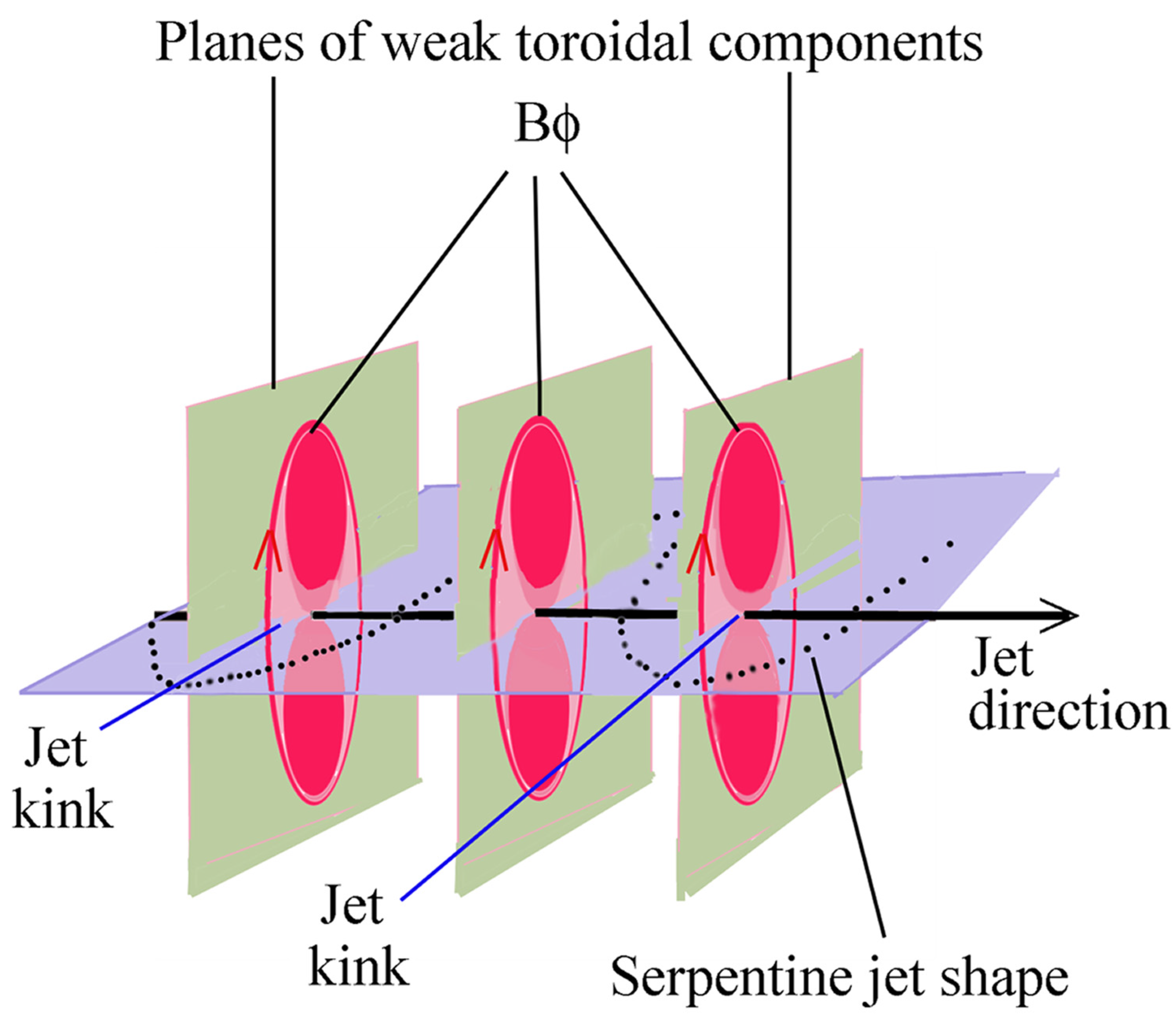
Various kinds of magnetized jet instability—including kink instability—are caused by the interplay of radial, azimuthal, and toroidal components of the magnetic field of the jet. The kinks evolve on the plasma jet at the places where the toroidal B_φ component of the magnetic field becomes weak. In this scenario, the jet is confined by a toroidal magnetic field and accelerated outwards by the magnetic fields [5]. The kink instabilities are stabilized by high jet velocity, meaning that instabilities alter the jet orientation, but do not disrupt the overall structure of the jet [5].We present the formation of the kink on the magnetized jet, which keeps its direction of propagation and takes the serpentine shape in the toroidal magnetic field (Figure 27).

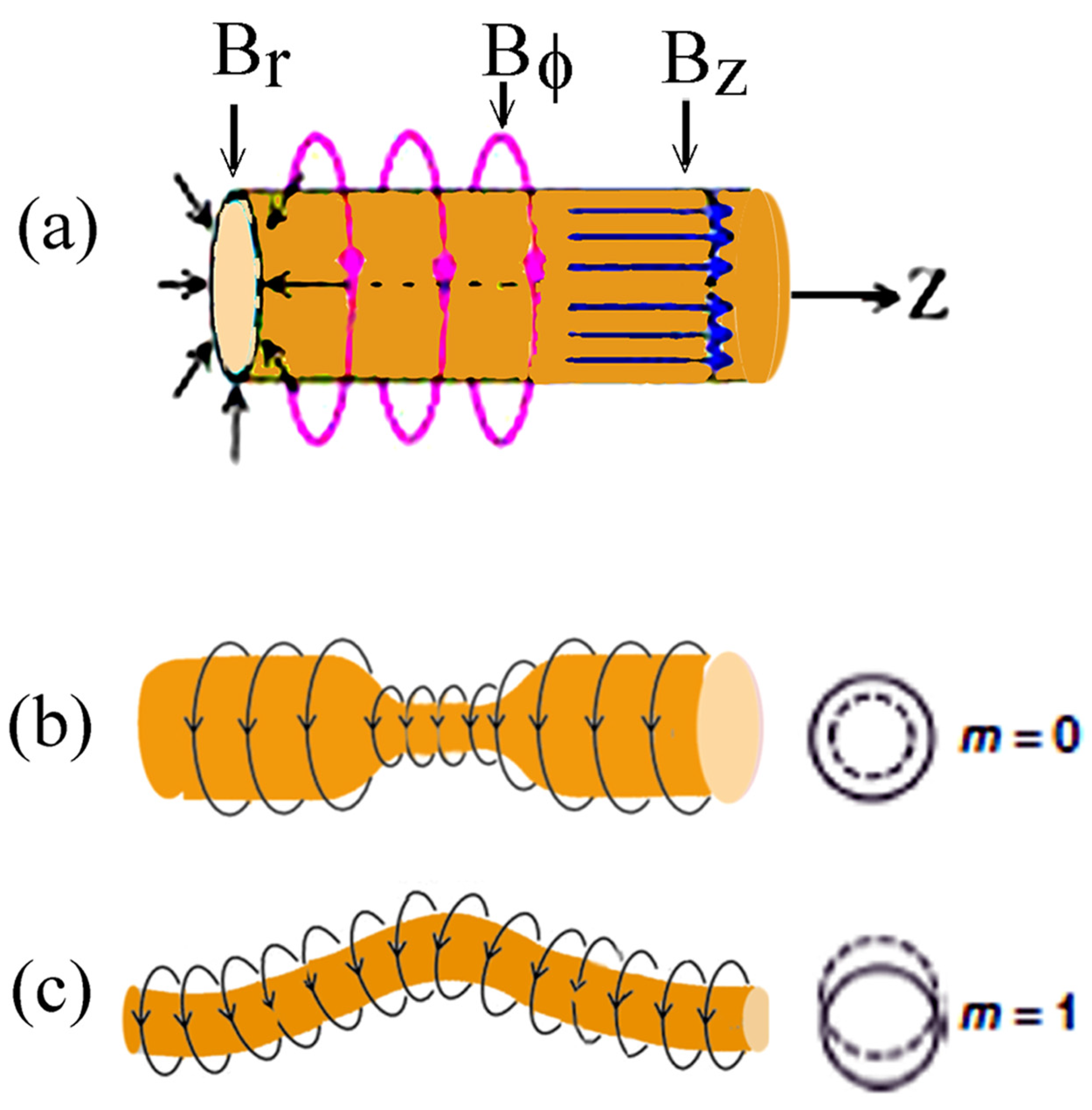
Magnetic field (B) of the jet consists of poloidal (B_p) and toroidal (B_ϕ) fields: B = B_p + B_ϕ, where B_p = B_R + B_z, i.e., the poloidal field consists of radial and azimuthal components as shown in Figure 28a.

Proton radio graphics revealed that the jet “is collimated throughout its propagation but has a sequence of clumps and changes of direction along its length. These features reflect perturbations in the magnetic field structure around the jet”; they grow locally and expand at each axial position, where the jet is unstable. The shape of the jet becomes serpentine due to the kink instability, creating a chain of kinks [5], and thus similar to that of the magnetized “South-East (SE) jet” of the Crab Nebula.

As concluded in [5], the jet filament shows two low-order fast-growing MHD current-driven instabilities with an increase in the B_ϕ toroidal component. Mode m = 0 is initiated by an increase in B_ϕ tension due to the radial contraction caused by vortex filament core thinning and the axis pinching when the criterion $\left|{\mathbf{B}}_{\phi }\right|>\left|{\sqrt{2|\mathbf{B}}}_{\mathrm{p}}\right|$ is fulfilled (Figure 28b). “Mode m = 1, kink, is initiated when the strength of the pressure B_ϕ increases at the inside of the kinks and decreases outside” [5] (Figure 28c). In that case, the product of toroidal and poloidal components becomes larger of some critical value α. The exact expression can be written as $\left|{\mathbf{B}}_{\phi }\right||{\mathbf{B}}_{\mathrm{p}}{|}^{-1}\lambda {(2\pi r_{\mathrm{j}})}^{-1}>\alpha$, where α is the criterion for the kink instability, λ is the jet modulation wavelength, and r_j is the radius [5].

Regarding the astrophysical plasmas where the expansion of plasmatic matter “can tend to stabilize the jet, resulting in α larger than of order unity. The plasma jet is stabilized when the magnetic field is overwhelmed by the parallel components as the toroidal components around the jet are too weak to excite the MHD instability. When the field is sufficiently large and has nonuniform toroidal components B_φ, current driven MHD kinks are excited” [5].

The fields are embedded in (“frozen-in”) and advected with the fast-moving magnetized plasma flow and give an insight into the kink instability evolution on the South-East Crab jet. According to Li et al. [5], “the plasmatic vortex filament-jets are caused by current-curing magnetic filaments in which spontaneously formed currents, magnetic fields, and plasma flow vectors are all collinear”. It is important to emphasize that in the laser-generated plasma, the jet kink instabilities are stabilized by high jet velocity, meaning that instabilities alter the jet orientation, but do not disrupt its overall structure—in agreement with the jet characteristics of the South-East Crab jet [5].

Therefore, the kink mode on the magnetized jet—which is similar to the bump—is initiated when the strength and pressure of B_φ increase at the inside of the kinks and decrease outside.

8. Double-Helix Nebula: Formation of Filament “Complex”

Different filamentary organization—a double-helix “complex”—at the astrophysical scale can be seen in the image of a Double-Helix Nebula (DHN), which is an infrared (IR) emission nebula created by filaments of ionized molecular gasses and dust, which under torsional magnetic field form a double-helix spiral similar to DNA molecule (Figure 29).

This feature is understood as a torsional Alfvén wave propagating from the Galactic disk and driven by rotation of the magnetized circumnuclear gas disk. It is proposed that the DHN is a hydrodynamic torsional Alfvén wave propagating vertically out of the Galactic plane, along magnetic field lines, from the near vicinity of the Galactic center [106] (Figure 29).

The IR image of the nebula is colored to be observed in visible light. The nebula is about ~80 ly long and at 300 ly from the huge black hole thought to be at the galaxy’s center. The formation of a double-helix shape of the nebula is caused by twisting magnetic field lines originating at the center of the Milky Way Galaxy, where the magnetic fields are extremely strong. Magnetic lines of this field are oriented perpendicular to the plane of the galaxy. It is speculated that these strong magnetic fields are created by the massive disc of gas circulating around the central supermassive black hole. This huge disk of gas (which orbits the black hole once every 10,000 years) is known as the circumnuclear disk (CND). It is strongly magnetized, and its predominant shear-induced azimuthal field is believed to merge with the ambient vertical galactic center field [107,108,109] The magnetic field lines are anchored in the CND and assumed to be the origin of the twisting of the magnetic field lines. These lines that are twisted at their base send a torsional wave in space. The magnetic field lines affect the orbits of molecular clouds and direct wind of hot gas and dust particles away from the central region. This twisting torsional wave carrying small dust particles and propagating very fast (about 1000 km/s) creates filaments that can absorb and emit infrared radiation giving rise to the Double-Helix Nebula shape. According to Morris et al. [106] the emission from the double helix most probably arises from thermal dust emission and molecular gas composition of filaments. The best-fit color temperature is ~630 K, while the thermal emission from dust gives ~410 K [106].

Large magnification of the image in Figure 29 reveals loops and kinks on the gaseous filament strands that make a double helix. Magnification reveals that filament strands are not long single filaments but eventually a group of filaments—“filament clusters”. Even more, some of the tiny filaments in the clusters are not firmly and closely incorporated into the common structure, but although slightly shifted—they follow the same organization principle. Thus, the “filaments” may eventually be taken as “filament clusters”, so that Double-Helix Nebula may be assumed a double-helix structure of filament clusters.

The double helix of vortex filament bundles (DHV)—which resembles the Double-Helix Nebula (DHN) of filament clusters—can be created by multipulse interaction of intense power laser with a Co-coated steel target. While the filament cluster in DHN is formed of “cold” dust particles at T = 400–600 K along helical magnetic lines, the DHV is formed by helical twisting of very hot fluid at T~10⁴ K. Although these double helix structures are created by quite different physical processes, they form plasmatic structures and their self-organization with the same (or similar) morphological and topological characteristics.

9. Formation of Complex Filamentary Structures in LMI

The double helix of vortex filament bundles can be created by the multipulse interaction of an intense power laser with a Co-coated steel target on a parallel scratched target surface. Such surface creates initial conditions with multimodal perturbation of the shear layer, which behaves, in a certain stage of the nanosecond LMI, like viscoelastic fluid. Normal stress difference in shearing flows is a fundamental property of viscoelastic fluids [105] The long filaments and ribbons with strongly anisotropic order parameter texture within the vortex sheet are characteristic of the anisotropic fluid mobility and are consistent with driving oscillatory strain field. This strain field changes in intensity and topology with the number of pulses N and causes a cascade of vortex filament and ribbon transformations [60,105]. Oscillatory strain fields cause motion and self-organization of filaments into helically paired, braided, and tangled patterns with topological complexity depending on the filament–filament separation distance and on the number of pulses. Interaction of vortex filaments with these strain fields generates various complex structures—“complexes”—in different regions of the target. Generation of localized coherent filamentary structures associated with turbulent mixing is a general phenomenon in accelerated flow environments from the atomic to nano-and micro-scales up to astrophysical scale as a result of nonlinear and nonequilibrium dynamics.

9.1. Helically Paired, Braided, and Tangled Structures of Vortex Filaments in LMI

Vortex filament bundles in Double-Helix Nebula organized along the helical magnetic field lines are very similar to double-helix vortex filament structures created by the power laser on the Co-coated steel target in the areas of a high density of vortex filaments. Under twisting, an array of closely packed parallel vortex filaments creates helices, double helices, and braided and tangled “complexes” such as the one shown in the center of Figure 30.

Helically paired and braided vortex filaments generated by multiple LMI are more complex self-organized structures than those generated by the single-pulse interaction. In fact, the first pulse in a series generates vortex filaments in a parallel array or the unbraided braid in the terminology of Tufillaro et al. [110] The subsequent pulses cause motion of vortex filaments, which results in braiding, the complexity of which varies over the interaction space. Vortex filaments generated in some surface region either loop through the surface to the position of another filament or simply step to it and continue in the same direction to another surface element. As these filaments are forced to move about each other under a series of laser pulses, the loops become entangled with the same topological structure. In many cases, a set of vortices intervene with each other while staying more or less parallel. At some places, fast reconnection and axial merging of nearby filaments disturb the topologic structure. Thus, filament dynamic is inhomogeneous in the interaction space during multipulse LMI, creating the complex double-helix structure of many vortex filament bundles, which actually reveals all the above-mentioned interactions as can be seen in Figure 31a.

In the above figure, one can identify the 3D vortex reconnection process seen at various stages as well as the series of vortex solitons. To analyze these structures, taking into account all involved processes would be an enormous task. Very idealized theoretical work has to be performed to relate these structures to vortex filaments and their multistage evolutions. This approach ignores (for simplicity) many physical processes, e.g., shock wave baroclinic vortex deposition, viscous dissipative processes, thermal transport, and change of state. However, a simplified approach enables insights into the structure of this “complex” and enables its topological analysis with transformation, which represents it—in the mathematical sense—by the irreducible braid.

Vortex filaments in bundles are very close and tend to axial merging with diffuse core spreading. However, some filaments that are slightly separated from the bundles make a series of random loops, kinks, and other deformations, which—due to diffuse core spreading—appear misty. Approximate reconstruction of this “complex”—assuming that the core size of individual filaments is σ ~5–6 μm—reveals 10–11 vortex filaments organized into 5 bundles (Figure 31b).

The reconstruction reveals that some filaments that form bundles at a larger distance become split and then joined to another bundle. An example is the bundle composed of light-blue and dark-blue filaments, which are very close to the left side; approaching the right side of the diagram, this bundle becomes separated into two independent bundles that have different pairing dynamics. Similar behavior can be seen on the black bundle, which after the formation of two loops also splits into two different bundles (Figure 31b).

9.2. Topological Transformations of Braided Vortex Filaments

To analyze the characteristics of a double helix in the reconstructed braid of vortex-filament strings in Figure 31b, the topological operations should be applied to reach the “irreducible structure of the braid”. Successive operations start with untwist—called the Reidemeister move type I—which gives the new braid. The next operations, pulling apart and sliding through the middle—Reidemeister moves II and III, respectively—result in the final braid diagram. These different planar diagrams of the same knot represent topologically equivalent knots [110,111]. Reidemeister moves of types I, II, and III simplify the study of knot equivalence by reducing it to a two-dimensional problem. The type I move untwists a section of a string, the type II move pulls apart two strands, and the type III move acts on three strings sliding the middle strand between the outer strands [110,111].

According to the braid theory, any oriented link of the strings can be represented by a closed braid. The identification between links, braids, and the braid group allows us to pass back and forth between the geometric braids and the algebraic braid group. A geometric braid is constructed between two level lines with n base points chosen on these level lines. If the i + 1st strand passes over the i-th strand, there is a positive crossing between the two strands. An overcrossing (or right-crossing) between the i + 1st and i-th string is denoted by the symbol σ_i. The inverse σ_i⁻¹ represents an undercross (or left-cross), i.e., the i + 1st strand goes under the i-th strand.

A general n-braid can be built up from successive applications of the operators σ_i and σ_i⁻¹. The first crossing between the second and third strands is represented by the operator σ₂. The next crossing between the third and fourth strands is negative, σ₃⁻¹, while the last crossing is represented by the operator σ. Each geometric diagram for a braid is equivalent to an algebraic braid word constructed from the overcrossing and undercrossing operators. The construction of a braid word is based on the following conventions. In each operation (σ_i,σ_i⁻¹), only the i-th and i + 1st strands are involved—not any other; it is not the string, but the base point which is numbered [110,111]. By the application of these topological operations, the reconstructed braid in Figure 31b is first—by the untwist operation—transformed into the new equivalent geometric braid (Figure 32a). The successive operations, pulling apart and sliding through the middle, transform this braid into another new equivalent braid (Figure 32b). Finally, the identification of overcrossings σ_i and undercrossings σ_i⁻¹ of the strings in this diagram makes it possible to construct the algebraic braid word.

Figure 32c shows the final reconstruction of the braid “complex” with 35 over- and undercrossings of five strings represented by the algebraic braid word.

σ₂σ₃σ₁σ₂⁻¹σ₁⁻¹σ₂σ₁σ₁⁻¹σ₂σ₃σ₁⁻¹σ₄σ₂σ₃⁻¹σ₁σ₄⁻¹σ₁⁻¹σ₄σ₁σ₄⁻¹σ₂σ₁⁻¹σ₃σ₃⁻¹σ₁σ₁⁻¹σ₁σ₃⁻¹σ₂σ₄⁻¹σ₃⁻¹σ₄σ₂σ₃σ₄⁻¹

(23)

Since braiding is not homogeneous, the strings (4,1) and (4,2) form (irregularly) alternating segments of dense and rare helical pairing, while the string (5) is not paired except with the string (1).

Having identified braid words and transferring them into matrix form (matrix representation of braid) enable one to define the set of differential equations, which describe filament dynamics. This would be a serious task for the braid (23) because its structure does not offer the possibility for the formation of smaller simple block matrices. Namely, helical pairing alternates with variable phase and wavelength along the braid axis; a dense and rare pairing alternate in opposite phases somewhat irregularly, so that the braid (Figure 32b,c) is not symmetric, and its theoretical consideration is out of the scope of this paper.

However, we can mention some important topological characteristics of such braids. The topological structure of braided vortex filaments is created by their twisting caused by vertical motions. Because twist commutes with other structures, the opposite senses of twist on a tube cancel [112] The crucial role is played by the commutativity of twist and the relaxation of braids into minimal patterns—irreducible topologic structures [111,112]. “Uniform twists commute with all other braid structures. However, more complex braid structures generally do not commute. In principle, the structures do have same freedom to relax to minimal patterns -irreducible structures, corresponding to minimum energy states” [112].

The braids generated by multipulse LMI are mostly random braids frozen (solidified) in a turbulent state, i.e., not in the state of the minimum energy [111,112]. It happens that the flux within one element can break, loose, and wander across the surface, but not far from its original location. If the elements break up and reform before the sequence of vorticity changes sign, then the twist will be trapped within a more complicated braid structure, preventing cancelation [111,112].

With regard to the micrograph shown in Figure 31a, it can be analyzed and described at two levels: (i) at the level of filaments of decomposed braids and represented by the irreducible graph in Figure 32b,c and (ii) at the level of braids which are helically paired giving rise to the double-helix structure similar to that of the Crab Nebula.

10. Conclusions

This study of plasma instabilities brings together the results of LMI at the microscale and plasmatic structures in astrophysical systems at the megascale. Demonstrating a variety of plasma fluid flow instabilities in LMI, their morphologic and topologic characteristics are used as a reference for the classification of similar megascale instabilities in the Crab Nebula and Double-Helix Nebula.

Using multipulse laser interaction, we created plasma-fluid-layer instability, which resulted in the formation of RTI, vortex filaments, loop solitons, and the loop-soliton chains on vortex filaments. They are similar to those in the near peripheral region of the Crab Nebula, where the loop-soliton chains evolve due to helicoidal magnetic field lines.

We found that the same Hasimoto-type function that describes the formation of the loop solitons (caused by torsion of vortex filaments) also describes the formation of the loop solitons on magnetized plasma filaments (caused by helical winding of magnetic field lines) in the NPR of the Crab Nebula.

Our findings reveal that multipulse laser irradiation causes breakup of the loop solitons, creates vortex rings, and creates four types of vortex ring instabilities. We demonstrate, for the first time, that morphological and topological characteristics of these ring instabilities at the microscale are similar to those at the megascale and establish the conceptual frame for their unique classification based on the hierarchical order of Bessel functions. This classification reveals that two types of vortex ring instabilities belong to the parametric resonance of helicoidal modes, while the other two are a combination of quasistatic deformation modes of Kelvin waves on the vortex ring. We also demonstrate that although all four types of instabilities are present, only the bulge wave is dominant in the peripheral region of the Crab Nebula.

Our results also demonstrate that multipulse LMI may create a quite different type of instability, critically depending on the filament–filament distance. Governed by the characteristics of the plasma–fluid layer, where the vortex filament distance is small (about one core radius), the instability is initiated leading to the formation of braids and helical pairing. In such regions, the created conditions favor the motion of vortex filaments close to each other, leading to the onset of collective behavior and the formation of bundles. Subjected to twisting and torsional strain fields, bundles become helically paired while some—almost free vortex filaments in the bundles—form loop solitons creating “complexes”. The formation and behavior of filament-bundle “complexes” in the shock-induced environment are described for the first time. We also show that these complexes are very similar to the magnetized jet filaments, filament bundles, and helically paired bundles—actually clusters—in the near central region of the Crab Nebula. Strong MHD radial and azimuthal instabilities on the filament jets in the bundles cause the formation of kinks, open loops, rings, and ring instabilities in the Crab Nebula.

Our overall findings show that the evolution of complexes may create a variety of filamentary architectures. Some of the complexes of closely packed vortex filaments tend to form a double-helix structure (DHS), which may be compared with a Double-Helix Nebula (DHN) bundle structure. Topological transformations of (symmetric) double-helix bundles lead to the irreducible braid graph, which reveals that DHN is actually the braided filamentary structure of much lower symmetry.

References

- Anisimov, S.I.; Drake, R.P.; Gauthier, S.; Meshkov, E.E.; Abarzhi, S.I. What is certain and what is not so certain in our knowledge of Rayleigh–Taylor mixing? Philos. Trans. R. Soc. A 2013, 371, 20130266. [Google Scholar] [CrossRef]
- Zhou, Y. Rayleigh–Taylor and Richtmyer–Meshkov instability induced flow, turbulence, and mixing. I. Phys. Rep. 2017, 720–722, 1–136. [Google Scholar] [CrossRef]
- Zhou, Y. Rayleigh–Taylor and Richtmyer–Meshkov instability induced flow, turbulence, and mixing. II. Phys. Rep. 2017, 723–725, 1–160. [Google Scholar] [CrossRef]
- Abarzhi, S.I.; Bhomwick, A.K.; Naveh, A.; Pandian, A.; Swisher, N.C.; Stellingwerf, R.F.; Arnett, W.D. Supernova, nuclear synthesis, fluid instabilities, and interfacial mixing. Proc. Natl. Acad. Sci. USA 2017, 116, 18184–18192. [Google Scholar] [CrossRef]
- Li, C.K.; Tzeferacos, P.; Lamb, P.; Gregori, D.; Norreys, G.; Rosenberg, P.; Follett, M.; Froula, R.; Koenig, D.; Seguin, M.; et al. Scaled laboratory experiments explain the kink behavior of the Crab Nebula jet. Nat. Commun. 2016, 7, 13081. [Google Scholar] [CrossRef]
- Gonoskov, A. Ultraintense Laser-Plasma Interaction for Applied and Fundamental Physics. Ph.D. Thesis, UMEA University, Umea, Sweeden, 2014. [Google Scholar]
- Kabashin, A.V.; Delaporte, P.; Grojo, D.; Torres, R.; Sarnet, T.; Sentis, M. A Review on Metal Nanostructures: Preparation Methods and Their Potential Applications. Nanoscale Res. Lett. 2010, 5, 454–463. [Google Scholar] [CrossRef]
- Lorazo, P.; Lewis, L.J.; Meunier, M. Short-pulse laser ablation of solids: From phase explosion to fragmentation. Phys. Rev. Lett. 2003, 91, 225502. [Google Scholar] [CrossRef]
- Rai, V.N.; Thakur, S.N. Ch.4—Physics and dynamics of plasma in laser-induced breakdown spectroscopy. In Laser Induced Breakdown Spectroscopy, 2nd ed.; Elsevier: Amsterdam, The Netherlands, 2020; pp. 71–106. [Google Scholar] [CrossRef]
- Anabitarte, F.; Cobo, A.; Lopez-Higuera, J.M. Laser-Induced Breakdown Spectroscopy: Fundamentals, Applications, and Challenges. Int. Sch. Res. Not. 2012, 2012, 285240. [Google Scholar] [CrossRef]
- Lugomer, S. Laser-Matter Interactions: Surface Self-organization; Profil International, Ed.; Profil International: Zagreb, Croatia, 2001. [Google Scholar]
- Zabusky, N.J.; Lugomer, S.; Zhang, S. Micro-fluid dynamics via laser metal surface interactions: Wave-vortex interpretation of emerging multiscale coherent structures. Fluid Dyn. Res. 2005, 36, 291–299. [Google Scholar] [CrossRef]
- Harillal, S.; Bindhu, C.V.; Tillack, M.S.; Najmabadi, F.; Gaeris, A.C. Internal structure and expansion dynamics of laser ablation plumes into ambient gases. J. Appl. Phys. 2003, 93, 2380–2387. [Google Scholar] [CrossRef]
- Dzhibladze, M.I.; Melikishvili, Z.G.; Berdzenishvili, L.E. The Interaction of Photon Clusters with Matter. Laser Phys. 2000, 10, 727–729. [Google Scholar]
- Ma, Q.I.; Motto-Ros, V.; Boueri, M.; Bai, X.S.; Zheng, L.J.; Zheng, H.P.; Yu, J. Temporal and spatial dynamics of laser-induced Al plasma in Ar background at atmospheric pressure: Interplay with the ambient gas. Spectrocim. Acta Part B 2010, 65, 896–907. [Google Scholar] [CrossRef]
- Matsumoto, J.; Masada, Y. Two-dimensional numerical study for Rayleigh-Taylor and Richtmyer-Meshkov instabilities in relativistic jets. Astrophys. J. 2013, 772, L1. [Google Scholar] [CrossRef]
- Lugomer, S. Laser generated Richtmyer-Meshkov instability and nonlinear wave paradigm in turbulent mixing: I. Central region of Gaussian spot. Laser Part. Beams 2016, 34, 687–704. [Google Scholar] [CrossRef]
- Lugomer, S. Laser generated Richtmyer-Meshkov instability and nonlinear wave paradigm in turbulent mixing: II. Near-Central region of Gaussian spot. Laser Part. Beams 2017, 35, 210–225. [Google Scholar] [CrossRef]
- Lugomer, S. Laser generated Richtmyer-Meshkov and Rayleigh-Taylor instabilities: III. Near/peripheral region of Gaussian spot. Laser Part. Beams 2017, 35, 597–609. [Google Scholar] [CrossRef]
- Boustie, M.; Berthie, L.; de Resseguier, T.; Arrigoni, M. Laser Shock Waves: Fundamentals and Applications. In Proceedings of the 1st International Symposium on Laser Ultrasonics: Science, Technology and Applications, Montreal, QC, Canada, 16–18 July 2008. [Google Scholar]
- Sundarapandian, S. Strong Blast Wave Interaction with Multiphase Media; Technical Report; Royal Institute of Tchnology, Department of Mechanics: Stockholm, Sweden, 2018; Available online: https://www.diva-portal.org/smash/get/diva2:1207069/FULLTEXT02.pdf (accessed on 26 December 2023).
- Devaux, D.; Fabbro, R.; Virmont, J. Generation of shock waves by laser-matter interaction in confined geometries. J. Phys. IV Proc. 1991, 1, C7-179–C7-182. [Google Scholar] [CrossRef]
- Petzolt, S.; Reif, J.; Matthias, E. Laser plasma threshold of metals. Appl. Surf. Sci. 1996, 96–98, 199–204. [Google Scholar] [CrossRef]
- Fabro, R.; Fournier, R.; Ballard, P.; Devaux, D.; Virmont, J. Physical study of laser-produced plasma in confined geometry. J. Appl. Phys. 1990, 68, 775–784. [Google Scholar] [CrossRef]
- Raizer, Y.P. Subsonic propagation of alight spark and threshold conditions for the maintenance of plasma by radiation. Sov. Phys. JETP 1970, 31, 1148–1154. [Google Scholar]
- Benselama, A.; Mame, W.-I.; Monnoyer, F. A 1D–3D mixed method for the numerical simulation of blast waves in confined geometries. J. Comput. Phys. 2009, 228, 6796–6810. [Google Scholar] [CrossRef]
- Carter, J.; Pathikonda, G.; Jiang, N.; Felver, J.J.; Ranjan, D. Time-resolved measurements of turbulent mixing in shock driven variable density flows. Nat. Sci. Rep. 2019, 9, 20315. [Google Scholar] [CrossRef] [PubMed]
- Lombardini, M.; Hill, D.J.; Pullin, D.I.; Meiron, D.I. Atwood ratio dependence of Richtmyer–Meshkov flows under reshock conditions using large-eddy simulations. J. Fluid Mech. 2001, 670, 439–480. [Google Scholar] [CrossRef]
- Zhou, Y.; Cabot, W.H. Time-dependent study of anisotropy in Rayleigh-Taylor instability induced turbulent flows with a variety of density ratios. Phys. Fluids 2019, 31, 084106. [Google Scholar] [CrossRef]
- Zabusky, N.J. Vortex paradigm for accelerated inhomogenous flows: Visiometrics foer the Rayleigh-Taylor and Richtmyer-Meshkov instabilities. Annu. Rev. Fluid Mech. 1999, 32, 495–536. [Google Scholar] [CrossRef]
- Schiling, O.; Latini, M.; Don, W.S. Physics of reshock and mixing in single-mode Richtmyer-Meshkov instability. Phys. Rev. E 2007, 76, 026319. [Google Scholar] [CrossRef] [PubMed]
- Schilling, O.; Jacobs, J.F. Richtmyer-Meshkow instability and re-accelerated inhomogenous flows. Scholarpedia 2008, 3, 6090. [Google Scholar] [CrossRef]
- Zhou, Y.; Cabot, W.H.; Thornber, B. Asimptotic behavior of the mixed mass in Rayleigh-Taylor and Richtmyer-Meshkow instabity induced flows. Phys. Plasmas 2016, 23, 052712. [Google Scholar] [CrossRef]
- Banerjee, A. Rayleigh-Taylor instability: A status review of experimental designs and measurement diagnostics. J. Fluids Eng. 2020, 142, 120801. [Google Scholar] [CrossRef]
- Roberts, M.S.; Jacobs, J.W. The effects of forced small-wavelength, finite-bandwidth initial perturbations and miscibility on the turbulent Rayleigh–Taylor instability. J. Fluid Mech. 2015, 787, 50–83. [Google Scholar] [CrossRef]
- Miles, A.R.; Blue, B.; Edwards, M.J.; Greenough, J.A.; Hansen, F.; Robey, H.; Drake, R.P.; Kuranz, C.; Leibrandt, R. Transition to turbulence and effect of initial conditions on 3D compressible mixing in planar blast-wave-driven systems. Phys. Plasmas 2005, 12, 056317. [Google Scholar] [CrossRef]
- Hill, D.L.; Abarzhi, S.I. On the RT unstable dynamics of 3D interfacial coherent structures with time-dependent acceleration. AIP Adv. 2019, 9, 075012. [Google Scholar] [CrossRef]
- Hill, D.L.; Abarzhi, S.I. Richtmyer-Meshkow dynamics with variable acceleration by group theory approach. Appl. Math. Lett. 2020, 105, 106338. [Google Scholar] [CrossRef]
- Bhowmick, K.; Hill, D.L.; Matthews, M.; Abarzhi, S.I. On the fundamentals of Richtmyer Meshkov dynamics with variable acceleration. arXiv 2019, arXiv:1902.01246. [Google Scholar]
- Abarzhi, S.I. Special class od self-similar dynamics for Rayleigh-Taylor mixing with variable acceleration. arXiv 2019, arXiv:1901.04563. [Google Scholar]
- Bhomwick, A.K.; Abarzhi, S.I. Richtmyer-Meshkov unstable dynamics influenced by pressure fluctuation. Phys. Plasmas 2016, 23, 112702. [Google Scholar] [CrossRef]
- Abarzhi, S.I. Coherent structures and pattern formation in Rayleigh-Taylor turbulent mixing. Phys. Scr. 2008, 78, 015401. [Google Scholar] [CrossRef]
- Pandian, A.; Stellingwerf, R.F.; Abarzhi, S.I. Effect of elative phase of waves constituting the initial perturbation and the wave interference in the dynamics of strong-shock-driven Richtmyer-Meshkov flows. Phys. Rev. Fluids 2017, 2, 073903. [Google Scholar] [CrossRef]
- Hoefer, M.; Ablowitz, M. Dispersive shock waves. Scholarpedia 2009, 4, 5562. [Google Scholar] [CrossRef]
- Koepke, M.E. Interrelationship between Lab, Space, Astrophysical, Magnetic Fusion, and Inertial Fusion Plasma Experiments. Atoms 2019, 7, 35. [Google Scholar] [CrossRef]
- Morace, A.; Abe, Y.; Honrubia, J.J.; Iwata, N.; Arikawa, Y.; Nakata, Y.; Johzaki, T.; Yogo, A.; Sentoku, Y.; Mima, K.; et al. Super-strong magnetic field-dominated ion beam dynamics in focusing plasma devices. Sci. Rep. 2022, 12, 6876. [Google Scholar] [CrossRef] [PubMed]
- Theobald, W.; Wũlker, C.; Jasny, J.; Bakos, J.S.; Jethwa, J.; Schaffer, F.P. High-density lithium plasma columns generated by intense subpicosecond KrF laser pulses. Opt. Commun. 1988, 149, 289–295. [Google Scholar] [CrossRef]
- Levescue, J.M. Magnetized, Laser-Driven, Plasma Experiments at Astrophysically Relevant Conditions, and Proton Imaging of Magnetic Fields. Ph.D. Thesis, The University of Michigan, Ann Arbor, MI, USA, 2020. [Google Scholar]
- Stamper, J.A. Review on spontaneous magnetic filelds in laser-produced plasmas: Phenomenaand measurements. Laser Part. Beams 1991, 9, 841. [Google Scholar] [CrossRef]
- Wilson, T.C.; Sheng, Z.-M.; Eliasson, B.; McKenna, P. Magnetic field magnification by high power lasers in underdanse plasma. Plasma Phys. Control. Fusion 2021, 63, 084001. [Google Scholar] [CrossRef]
- Gao, L.; Ji, H.; Fiksel, G.; Fox, W.; Evans, M.; Alfonso, N. Ultrafast proton radiography of the magnetic fields generated by a laser-driven coil current. Phys. Plasmas 2016, 23, 043106. [Google Scholar] [CrossRef]
- Goyon, C.; Pollock, B.B.; Turnbull, D.P.; Hazi, A.; Divol, L.; Farmer, W.A.; Haberberger, D.; Javedani, J.; Johnson, A.J.; Kemp, A.; et al. Ultrafast probng of magnetic field growth inside a laser-diven solenoid. Phys. Rev. E 2017, 95, 033208. [Google Scholar] [CrossRef] [PubMed]
- Santos, J.J.; Bailly-Grandvaux, M.; Giuffrida, L.; Forestier-Colleoni, P.; Fujioka, S.; Zhang, Z.; Korneev, P.; Bouillaud, R.; Dorard, S.; Batani, D.; et al. On the Nature of the Crab Nebula’s Optical Emission. Dokl. Akad. Nauk. SSSR 1953, 90, 983–986. [Google Scholar] [CrossRef]
- Law, K.F.F.; Bailly-Grandvaux, M.; Morace, A.; Sakata, S.; Matsuo, K.; Kojima, S.; Lee, S.; Vaisseau, X.; Arikawa, Y.; Yogo, A.; et al. Direct measurement of kilo-tesla magnetic filed gennerated wia laser-driven capacitor-coil target by proton deflectometry. Appl. Phys. Lett. 2016, 108, 091104. [Google Scholar] [CrossRef]
- Wanger, U.; Wagner, U.; Tatarakis, M.; Gopal, A.; Beg, F.N.; Clark, E.L.; Dangor, A.E.; Evans, R.G.; Haines, M.G.; Mangles, S.P.D.; et al. Laboratory measurements of 0.7 GG magnetic fields generated during high-intensity laser interactions with dense plasmas. Phys. Rev. E 2004, 70, 026401. [Google Scholar] [CrossRef]
- Longman, A.; Fedosejevs, R. Kilo-Tesla axial magnetic field generation with high intensity spin and orbital angular momentum beams. Phys. Rev. Res. 2021, 3, 043180. [Google Scholar] [CrossRef]
- Fukumoto, Y.; Lugomr, S. Instability of Vortex Filaments and Stabilization of Finite Core. Available online: https://repository.kulib.kyoto-u.ac.jp/dspace/bitstream/2433/43208/1/1326_03.pdf (accessed on 26 December 2023).
- Lugomer, S.; Fukumoto, Y. Hierarchical instability of vortex ring array in multipulse laser-matter interactins. Fluid Dyn. Res. 2005, 36, 277–290. [Google Scholar] [CrossRef]
- Fukumoto, Y.; Lugomer, S. Instability od vortex filaments in laser-matter interactions. Phys. Lett. 2003, 308, 375–380. [Google Scholar] [CrossRef]
- Lugomer, S.; Fukumoto, Y. Generation of ribbons, helicoids, and complex Scherk surfaces in laser-matter interactions. Phys. Rev. E 2010, 81, 036311. [Google Scholar] [CrossRef] [PubMed]
- Lugomer, S.; Fukumoto, Y. Supercomplex network of bistable coiled vortex filaments and ribbons in laser-matter interactions. J. Mod. Appl. Phys 2018, 2, 1–9. [Google Scholar]
- Lugomer, S. Micro-fluid dynamics via laser–matter interaction: Vortex filament structures, helical instability, reconnection, merging, and undulation. Phys. Lett. A 2007, 361, 87–97. [Google Scholar] [CrossRef]
- Collis, S.S.; Lele, S.K.; Moser, R.D.; Rogers, N.M. The evolution of a plane mixing layer with spanwise nonuniform forcing. Phys. Fluids 1994, 6, 381–396. [Google Scholar] [CrossRef]
- Wu, J.-Z.; Ma, H.Y.; Zhou, M.-D. Vorticity and Vortex Dynamics; Springer: Berlin/Heidleberg, Germany, 2006. [Google Scholar]
- Nakayama, K.; Segur, H.; Wadati, M. Integrability and the motion of curves. Phys. Rev. Lett. 1992, 69, 2603–2606. [Google Scholar] [CrossRef] [PubMed]
- Maksimovic, A.; Lugomer, S.; Michieli, I. Multisolitons on vortex filaments: The origin of axial tangling. J. Fluids Struct. 2003, 17, 317–330. [Google Scholar] [CrossRef]
- Hereman, W.; Zhuang, W. Symbolic computation of solitons with Macsyma. In Proceedings of the 13th IMACS World Congress Dublin, Dublin, Ireland, 22–26 July 1991; Ames, W.F., van der Houwen, P.J., Eds.; pp. 287–296. [Google Scholar]
- Fukumoto, Y.; Moffatt, H.K. Motion and expansion of a viscous vortex ring. Part 1. A higher-order asymptotic formula for the velocity. J. Fluid Mech. 2000, 417, 1–45. [Google Scholar] [CrossRef]
- Fukumoto, Y.; Hattori, Y. Curvature instability of a vortex ring. J. Fluid Mech. 2005, 526, 77–115. [Google Scholar] [CrossRef]
- Fukumoto, Y. The three-dimensional instability of a strained vortex tube revisited. J. Fluid Mech. 2003, 493, 287–318. [Google Scholar] [CrossRef]
- Fukumoto, Y.; Hattori, Y. Linear stability of a vortex ring revisited. In Proceedings of the IUTAM Symposium on Tubes, Sheets and Singularities in Fluid Dynamics, Zakopane, Poland, 2–7 September 2001; Moffatt, H.K., Bajer, K., Eds.; Kluwer Academic Publishers: Dordrecht, The Netherlands, 2002; pp. 37–48. [Google Scholar]
- Hattori, Y.; Fukumoto, Y. Short-wavelength stability analysis of thin vortex rings. Phys. Fluids 2003, 15, 3151–3163. [Google Scholar] [CrossRef]
- Widnall, S.E.; Bliss, D.B.; Tsai, C.-Y. The instability of short waves on a vortex ring. J. Fluid Mech. 1974, 66, 35–47. [Google Scholar] [CrossRef]
- Widnal, S.E.; Tsai, C.Y. The instability of the thin vortex ring of constant vorticity. Philos. Trans. R. Soc. Lond. A 1977, 287, 273–305. [Google Scholar]
- Kop’ev, V.F.; Chernyshev, S.A. Vortex ring oscillations, the development of turbulence in vortex rings and generation of sound. Phys. Uspekhi 2000, 43, 663–690. [Google Scholar] [CrossRef]
- Abarzhi, S.I.; Goddard, W.A., III. Interfaces and mixing: Nonequilibrium transport across the scales. Proc. Natl. Acad. Sci. USA 2019, 116, 18171–18174. [Google Scholar] [CrossRef] [PubMed]
- Abarzhi, S.I.; Hill, D.L.; Williams, K.C.; Li, J.T.; Remington, B.A.; Arnett, W.D. Fluid Dynamic Mathematical Aspects of Supernova Remnants. Phys. Fluids 2023, 35, 034106. [Google Scholar] [CrossRef]
- Hester, J.J.; Loll, A. The Crab Nebula, Hubble’s Messier Catalog, Messier 1, NASA. 2017. Available online: https://science.nasa.gov/mission/hubble/science/explore-the-night-sky/hubble-messier-catalog/messier-1/ (accessed on 26 December 2023).
- Shklovskii, I. On the Nature of the Crab Nebula’s Optical Emission. Dokl. Akad. Nauk. SSSR 1953, 90, 983. [Google Scholar]
- Burn, B.J. A synchrotron model for the continuum spectrum of the Crab Nebula. Mon. Not. R. Astron. Soc. 1973, 165, 421–429. [Google Scholar] [CrossRef]
- Hester, J.J. The Crab Nebula: An Astrophysical Chimera. Annu. Rev. Astron. Astrophys. 2008, 46, 127–155. [Google Scholar] [CrossRef]
- Fesen, R.A.; Kirshner, R.P. The Crab Nebula. I—Strophotometry of the filaments. Astrophys. J. 1982, 258, 1–10. [Google Scholar] [CrossRef]
- Dubner, G.; Castelletti, G.; Kargaltsev, O.; Pavlov, G.G.; Bietenholz, M.; Talavera, A. Morphological Properties of the Crab Nebula: A Detailed Multiwavelength Study Based on New VLA, HST, Chandra, and XMM-Newton Images. Astrophys. J. 2017, 840, 82. [Google Scholar] [CrossRef]
- Mignone, A.; Striani, E.; Tavani, M.; Ferrari, A. Modelling the kink jet of the Crab Nebula. Mon. Not. R. Astron. Soc. 2013, 436, 1102–1115. [Google Scholar] [CrossRef]
- Lawrence, S.S.; MacAlpine, G.M.; Uomoto, A.; Woodgate, B.; Brown, L.W.; Oliversen, R.J.; Lowenthal, J.D.; Liu, C. Three-dimensional Fabry-Perot Imaging Spectroscopy of the Crab Nebula, Cassiopeia A, and Nova GK Persei. Astron. J. 1995, 109, 2635. [Google Scholar] [CrossRef]
- Kuranz, C.C.; Drake, R.P.; Grosskopf, M.J.; Drake, R.P.; Grosskopf, M.J.; Drake, R.P.; Grosskopf, M.J.; Fryxell, B.; Budde, A.; Hansen, J.F.; et al. Spike morphology in blast-wave-driven instability experiments. Phys. Plasmas 2020, 17, 052709. [Google Scholar] [CrossRef]
- Kuranz, C.C.; Park, H.-S.; Huntington, C.M.; Miles, A.R.; Remington, B.A.; Plewa, T.; Trantham, M.R.; Robey, H.F.; Shvarts, D.; Shimony, A.; et al. How high energy fluxes may affect Rayleigh–Taylor instability growth in young supernova remnants. Nat. Commun. 2018, 9, 1564. [Google Scholar] [CrossRef] [PubMed]
- Bietenholz, M.F.; Kronbberg, P.P. The Magnetic field of the Crab nebula and the nature of its “jet”. Astrophys. J. 1990, 357, L13–L16. [Google Scholar] [CrossRef]
- Tandberg-Hanssen, E. The Physics of Solar Flares; Cambridge University Press: Cambridge UK, 2009; Digitally Printed Version. [Google Scholar]
- Gaensler, B.M.; Slane, P.O. The evolution and structure of pulsar wind nebulae. Ann. Rev. Astron. Astrophys. ARA&A 2006, 44, 17–47. [Google Scholar] [CrossRef]
- Reynolds, S.P.; Gaensler, B.M.; Bocchino, F. Magnetic fields in supernova remnants and pulsar—Wind nebulae. Space Sci. Rev. 2012, 166, 231–261. [Google Scholar] [CrossRef]
- Mukherjee, D.; Bult, P.; van der Klis, M.; Bhattacharya, D. The magnetic-field strengths of accreting millisecond pulsars. Mon. Not. R. Astron. Soc. 2015, 452, 3994–4012. [Google Scholar] [CrossRef]
- Flowers, E.; Ruderman, M.A. Evolution of pulsar magnetic fields. Astrophys. J. 1977, 215, 302–310. [Google Scholar] [CrossRef]
- Hester, J.J.; Scowen, P.A.; Sankrit, R.; Lauer, T.R.; Ajhar, E.A.; Baum, W.A.; Code, A.; Currie, D.G.; Danielson, G.E.; Ewald, S.P.; et al. Hubble space telescope WFPC2 imaging of M16: Photoevaporation and emerging of young stellar objects. Astron. J. 1996, 111, 2349. [Google Scholar] [CrossRef]
- Lapenta, G.; Kronberg, P.P. Simultion of astrophysical jets: Collimation and expansion into radio lobes. Astron. J. 2005, 625, 37–50. [Google Scholar] [CrossRef]
- Andrade, L.C.G. Torsion effects on vortex filaments and Hasimoto soliton transformation in magnetar. arXiv 2005, arXiv:astro-ph/0509847. [Google Scholar]
- Ricca, R. Inflexional disequilibrium of magnetic flux-tubes. Fluid Dyn. Res. 2005, 36, 319. [Google Scholar] [CrossRef]
- Ricca, R. The effect of torsion on the motion pf a helical vortex filament. J. Fluid Mech. 1994, 237, 241. [Google Scholar] [CrossRef]
- Gull, T.R.; Fesen, R.A. Deep optical imagery of the Crab Nebula’s jet. Astrophys. J. 1982, 260, L75. [Google Scholar] [CrossRef]
- Sankrit, R.; Hester, J.J. The shock and extended remnant around the Crab Nebula. Astrophys. J. 1997, 491, 796–807. [Google Scholar] [CrossRef]
- Chevalier, R.A.; Gull, T.R. The outer structure of the Crab nebula. Astrophys. J. 1975, 200, 399–401. [Google Scholar] [CrossRef]
- Chevalier, R.A.; Fransson, C. Pulsar Nebulae in Supernovae. Astrophys. J. 1992, 395, 540–552. [Google Scholar] [CrossRef]
- Porth, O.; Komissarov, S.S.; Keppens, R. Rayleigh–Taylor instability in magnetohydrodynamic simulations of the Crab nebula. Mon. Not. R. Astron. Soc. 2014, 443, 547–558. [Google Scholar] [CrossRef]
- Clark, D.H.; Murdin, P.; Wood, R.; Gilmozzi, R.; Danziger, J.; Furr, A.W. Three-dimensional structure of the Crab Nebula. Mon. Not. R. Astron. Soc. 1983, 204, 415. [Google Scholar] [CrossRef]
- Becker, L.E.; Shelly, M.J. Instability of Elastic Filaments in Shear Flow Yields First-Normal-Stress Differences. Phys. Rev. Lett. 2001, 87, 198301. [Google Scholar] [CrossRef]
- Morris, M.; Uchida, K.; Do, T. A magnetic torsional wave near the Galactic Centre traced by a ‘double helix nebula’. Nature 2006, 440, 308–310. [Google Scholar] [CrossRef] [PubMed]
- Hildebrand, R.H.; Davidson, J.A.; Dotson, J.; Figer, D.F.; Novak, G.; Platt, S.R.; Tao, L. Polarization of the thermal emission from the dust ring at the center of the Galaxy. Astrophys. J. 1993, 417, 565–571. [Google Scholar] [CrossRef]
- Wardle, M.; Königl, A. A model for the magnetic field in the molecular disk at the Galactic center. Astrophys. J. 1990, 362, 120–134. [Google Scholar] [CrossRef]
- Novak, G.; Dotson, J.L.; Dowell, C.D.; Hildebrand, R.H.; Renbarger, T.; Schleuning, D.A. Submillimeter polarimetric observations of the galactic center. Astrophys. J. 2000, 529, 241–250. [Google Scholar] [CrossRef]
- Tufillaro, N.B.; Abott, T.; Reilly, J. An Experimental Approach to Nonlinear Dynamics and Chaos; Adison-Wesley Rub. Co.: New York, NY, USA; Amsterdam, The Netherlands, 1992. [Google Scholar]
- Lugomer, S. Braids of vortex filaments generated by laser on metal surface. Phys. Lett. A 1999, 259, 479–487. [Google Scholar] [CrossRef]
- Ricca, R.L.; Berger, M.A. Topological ideas and fluid mechanics. Phys. Today 1996, 49, 28–34. [Google Scholar] [CrossRef]
Figure 1.
Characteristics of laser-generated plasma on a solid target. Schematic diagram of expanding laser-produced plasma in a background gas. The plasma plume, first, expands vertically to the target; colored zones illustrate variations in temperature and density in the expanding plasma plume.
Figure 2.
Plasma spheroid expansion along the target surface. Plasma density distribution after radial expansion with the formation of characteristic regions below Gaussian laser power density distribution. Schematically, (a) a cross-section of the plasma spheroid in the (z,x) plane; lateral compression of background gas (air), and formation of the air shell (cocoon) around the plasma spheroid. (b) Formation of central minimum in the plasma density distribution due to expansion and compression of the background gas (ρ = plasma density; CR = central region; NCR = near central region; Y-direction is parallel to the target surface and perpendicular to the plane of the paper).
Figure 3.
Optical micrograph showing an array of parallel vortex filaments generated by N = 12 pulses, on a Co-coated steel target in the air, at the atmospheric pressure by XeCl laser with rectangular beam and the top hat profile; E = 0.25 J; τ = 16 ns (filament thickness ~5–7 μm; loop diameter 2R~28–30 μm).
Figure 4.
Loop soliton on vortex filament. Optical micrograph of the loop soliton on Cr-coated steel generated in the air (a); SEM micrograph of the loop soliton on Titanium target generated in vacuum (b).
Figure 5.
Optical micrograph of the chain of vortex filament loops (Hasimoto solitons) generated on Co-coated steel target.
Figure 6.
Two-soliton solution for k1 = 3, k2 = 1, t = −0.30 (a); t = −0.045 (b); t = 0.30 (c). Interaction of two loop solitons. Small loop soliton moving at high velocity approaches to the large slower one (a). Reaching the larger soliton, it becomes incorporated into the larger soliton (b); overtaking the large soliton, it continues to move at a higher velocity (c).
Figure 7.
Array of closely packed parallel quasi-periodic loop soliton chains—a quasiperiodic lattice. The strings are disturbed and indicate a tendency to catastrophic dynamics of the loop solitons after N = 12 to 13 pulses.
Figure 8.
Breakdown of 1D loop chain into a set of open loops and vortex rings on Co-coated steel target. Vortex rings after breakdown do not move much from the former positions in the string.
Figure 9.
Type I: Vortex ring instability identified as the “WBT instability”, parametric resonance between the left- and right-handed helical waves (m = ±1). The evolution of type I instability. The radius a of the core cross-section grows as (a) a~2.5 μm, and (b) a schematic illustration.
Figure 10.
Type II: Vortex ring instability identified as the “curvature instability”, parametric resonance between the helical (m = 1) and the bulge (m = 0) modes. This instability may be represented as a combination of the axisymmetric (m = 0) and the bending (m = 1) modes (a). A schematic illustration of this type of instability is shown in (b).
Figure 11.
Type III: Vortex ring oscillation identified as the Kelvin axisymmetric mode (m = 0). Schematic illustration (a–c) shows a standing deformation mode of the core as provided by Figure 10 of Kop’ev and Chernyshev [75]. Illustration (i–iv) shows the stages of the deformation mode.
Figure 12.
Type IV: (a) Vortex ring oscillation identified as the “standing deformation mode”, a combination of m = 0 and m = ±1 modes. (b) Schematic illustration from Figure 6b of Kop’ev and Chernysev [75].
Figure 13.
Optical micrograph showing a bundle of vortex filaments and a string of solitons created by laser on Co-coated steel (a). Rendering of (a) reveals the vortex filament “complex” showing multiloop solitons on bundles (b). While some vortex filaments are incorporated into bundles, those on the outer side of the bundles show individual motion.
Figure 14.
Schematic reconstruction of the vortex filament “complex” in Figure 14. Formation of two bundles of vortex filaments (i). Turbulent background field causes dense packing of filaments; twisting of bundles causes helical winding of individual bundles but also their helical pairing (ii). The peripheral filament in the bundle experiences additional torsion, which starts to form a series of loop solitons (iii). Closely packed filaments under the action of the surrounding turbulent background field experience core spreading and axial merging.
Figure 15.
Optical micrograph of vortex filament “complex” showing (+) and (−) soliton loops, filament coiling, and complex motion due to torsion and twisting fields.
Figure 16.
Reconstruction of the vortex filament “complex” in Figure 16 showing (+) and (−) soliton loops and filament coiling. Two connected rings represent the Hopf link created after loop soliton breakup and the formation of vortex rings. (a) The ring instability causes a breakup and anew connection with the nearest neighbor ring. (b) Schematic illustration of the interaction of (+) and (−) loop solitons (i) and their annihilation (ii).
Figure 17.
Optical micrograph of vortex filament “complex” showing the series of disarrayed Hasimoto solitons on two tangled vortex filaments. Small loop solitons are formed at the thin vortex filament separated from the thicker one. This indicates that thin and thick filaments under torsion have different dynamics although both form loop solitons. The structure is generated on the Co-coated-steel-plate in the air.
Figure 18.
Crab Nebulain the Taurus constellation(as the large mosaic of the Crab Nebula assembled from 24 individual exposures captured by Hubble Space telescope over three months). Image courtesy of NASA/ESA and Allison Loll/Jeff Hester (Arizona State University). Acknowledgment: Davide De Martin (ESA/Hubble).
Figure 19.
The upperright peripheral region of the Crab Nebula showing random loop solitons on magnetized vortex filaments. (Enlarged segment of the Crab Nebula in Figure 18. Image courtesy of NASA/ESA and Allison Loll/Jeff Hester (Arizona State University). Acknowledgment: Davide De Martin (ESA/Hubble).)
Figure 20.
The upperleft peripheral region of the Crab Nebula showing loop solitons in the chaotic organization of vortex filaments and diffusively spreaded cores of the vortex filaments. (Enlarged segment of the Crab Nebula in Figure 18. Image courtesy of NASA/ESA and Allison Loll/Jeff Hester (Arizona State University). Acknowledgment: Davide De Martin (ESA/Hubble).)
Figure 21.
Series of almost periodic loops on vortex filament (chain of the loop solitons) on the segment of the Crab Nebula. Vortex rings separated from the parent filament are seen in the vicinity. The picture is taken from the segment of the Crab Nebula. (Enlarged segment of the Crab Nebula in Figure 18. Image courtesy of NASA/ESA and Allison Loll/Jeff Hester (Arizona State University). Acknowledgment: Davide De Martin (ESA/Hubble).)
Figure 22.
The right peripheral region of the Crab Nebula. Broken filament loops and rings indicate the ring instability of type III (a,b); formation of clusters of vortex rings (c);and cluster of broken rings (d). (Enlarged segment of the Crab Nebula in Figure 18. Image courtesy of NASA/ESA and Allison Loll/Jeff Hester (Arizona State University). Acknowledgment: Davide De Martin (ESA/Hubble).)
Figure 23.
The double helix of gaseous magnetized bundles of filament jets in the near central region of the Crab Nebula. Some of the thin filament jets slightly separated from the bundles show the formation of loops. Filament jets are helically paired, and closed loops (similar to the loop solitons) are formed on a few filaments. (Enlarged segment of the Crab Nebula in Figure 18. Image courtesy of NASA/ESA and Allison Loll/Jeff Hester (Arizona State University). Acknowledgment: Davide De Martin (ESA/Hubble).)
Figure 24.
Enlarged details of Figure 23 showing vortex filament loops and rings on the filaments not firmly incorporated into the bundle, which manifest an individual behavior. (Enlarged segment of the Crab Nebula in Figure 18. Image courtesy of NASA/ESA and Allison Loll/Jeff Hester (Arizona State University). Acknowledgment: Davide De Martin (ESA/Hubble).)
Figure 25.
The double helix of magnetized tiny filaments, which connects the blue central part and the brown-yellow peripheral part in the Crab Nebula. Large magnification reveals small loops. (Enlarged segment of the Crab Nebula in Figure 18. Image courtesy of NASA/ESA and Allison Loll/Jeff Hester (Arizona State University). Acknowledgment: Davide De Martin (ESA/Hubble).)
Figure 26.
Near the central region of the Crab Nebula. Open loops, broken rings, and closed rings appearing with bundles of magnetic filament jets in the region of the very strong magnetic field. The ring instability (a) is similar to the type I parametric instability; the ring instabilities in (b,c) are similar to the type III, i.e., to the axisymmetric “bulge wave” (m = 0) that has reached the catastrophic limit and caused the ring breakdown. The instability (d) is similar to the vortex ring instability type IV of the long wavelength ring oscillations. The instabilities (e,f) do not correspond to the hierarchical ring instabilities but rather indicate the open loops. (Enlarged segment of the Crab Nebula in Figure 18. Image courtesy of NASA/ESA and Allison Loll/Jeff Hester (Arizona State University). Acknowledgment: Davide De Martin (ESA/Hubble).)
Figure 27.
Schematic of a plasma jet with the resulting toroidal magnetic field configuration. Plasma jet propagates in this magnetic field configuration with the formation of kinks that cause its serpentine shape. The kinks evolve at the places—in the planes—where the toroidal Bϕ component of the magnetic field is weak.
Figure 28.
Configuration of the self-generated, spontaneous magnetic field can be decomposed into poloidal (Bϕ = Br + Bz) and toroidal (Bϕ) components. (a) Schematic illustrations of the fastest growing MHD current-driven instabilities: mode m = 0, the core shrinking (sausage); (b) mode m = 0 (kink); (c) higher modes (m = 1).
Figure 29.
Double-Helix Nebula is the IR emission nebula in Sagittarius. The image was taken by the Multiband Imaging Photometer for Spitzer (MIPS). (Image courtesy of NASA/JPL-Caltech/M. Morris (UCLA). Acknowledgment: Steward Wolpert, UCLA.)
Figure 30.
Optical micrograph of a segment of vortex filaments that follow parallel surface scratches. Interaction between vortex filaments causes the formation of tangled filament bundles—the “complexes” (central region)—generated by XeCl laser on Co-coated steel by N = 13 pulses. Transversal oscillation causes motion and perturbation of filaments.
Figure 31.
The double helix of vortex filament bundles generated by XeCl laser on Co-coated steel: E = 0.25 J, N = 13, τ = 16–20 ns. Many filaments in the bundles are very close and show axial merging and the core spreading. Vortex filaments show strong diffuse core spreading in turbulent fields (a). Approximate reconstruction reveals ~11 vortex filaments organized into 5 tangled bundles, many of them with the loop solitons. A few bundles with distance from the left side show the splitting of some filaments, which then become part of another bundle (b).
Figure 32.
Topological reconstruction of vortex filament bundles organized into a braid and identification of the algebraic braid word. Application of topological operations untwist (Reidemeister move type I) creates the new braid (a). Subsequent operations pull apart and the middle slide (Reidemeister moves II and III) give the final braid shown in (b) with identified over- and undercrossings (c).
Disclaimer/Publisher’s Note: The statements, opinions and data contained in all publications are solely those of the individual author(s) and contributor(s) and not of MDPI and/or the editor(s). MDPI and/or the editor(s) disclaim responsibility for any injury to people or property resulting from any ideas, methods, instructions or products referred to in the content. |
© 2024 by the author. Licensee MDPI, Basel, Switzerland. This article is an open access article distributed under the terms and conditions of the Creative Commons Attribution (CC BY) license (https://creativecommons.org/licenses/by/4.0/).
Share and Cite
MDPI and ACS Style
Lugomer, S. Laser and Astrophysical Plasmas and Analogy between Similar Instabilities. Atoms 2024, 12, 23. https://doi.org/10.3390/atoms12040023
AMA Style
Lugomer S. Laser and Astrophysical Plasmas and Analogy between Similar Instabilities. Atoms. 2024; 12(4):23. https://doi.org/10.3390/atoms12040023
Chicago/Turabian StyleLugomer, Stjepan. 2024. "Laser and Astrophysical Plasmas and Analogy between Similar Instabilities" Atoms 12, no. 4: 23. https://doi.org/10.3390/atoms12040023
Note that from the first issue of 2016, this journal uses article numbers instead of page numbers. See further details here.