
Oxygen-Sensitive Metalloprotein Structure Determination by Cryo-Electron Microscopy

 , , and
Abstract
:1. Introduction
2. Materials and Methods
2.1. Protein Sample Preparation
2.2. Negative Staining
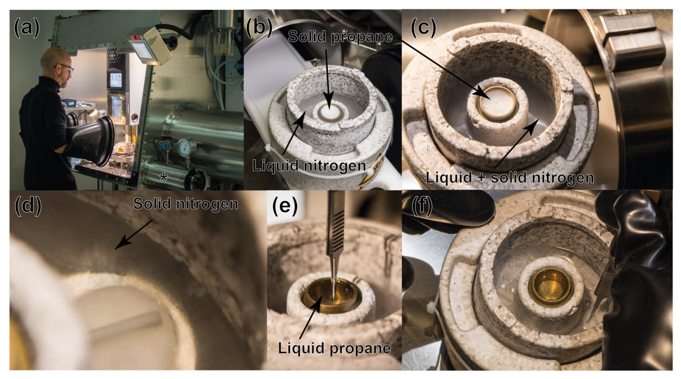
2.3. Cryo-EM Grid Preparation under Anaerobic Conditions
2.4. Cryo-EM Data Acquisition and Image Processing
2.4.1. Apoferritin
2.4.2. PFOR
2.5. Model Building in the Cryo-EM Maps
2.5.1. Apoferritin
2.5.2. PFOR
3. Results
3.1. Cryo-Electron Grids Preparation in Anaerobic Conditions
3.2. Protein Reconstructions
3.2.1. Apoferritin
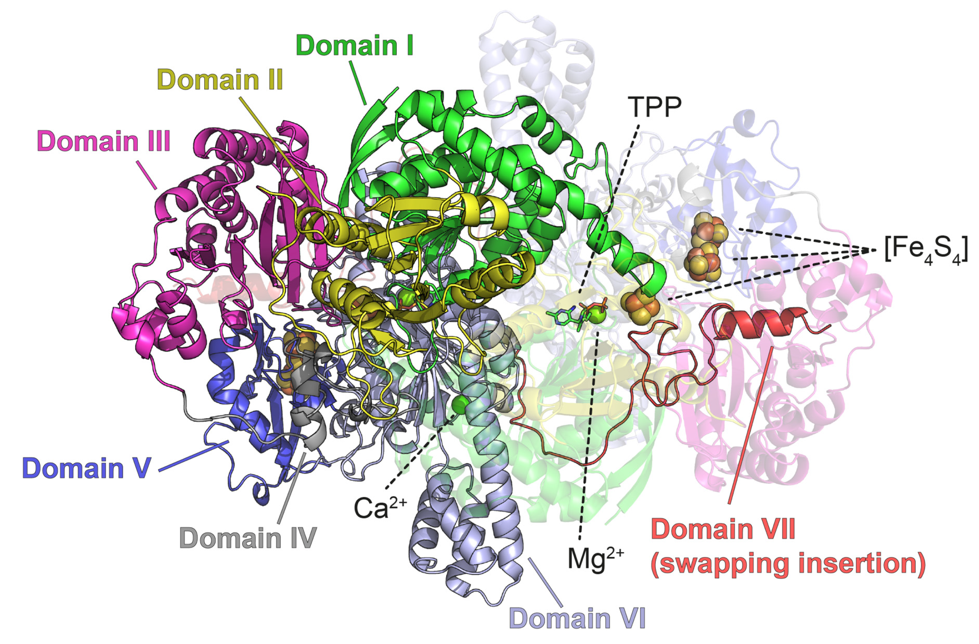
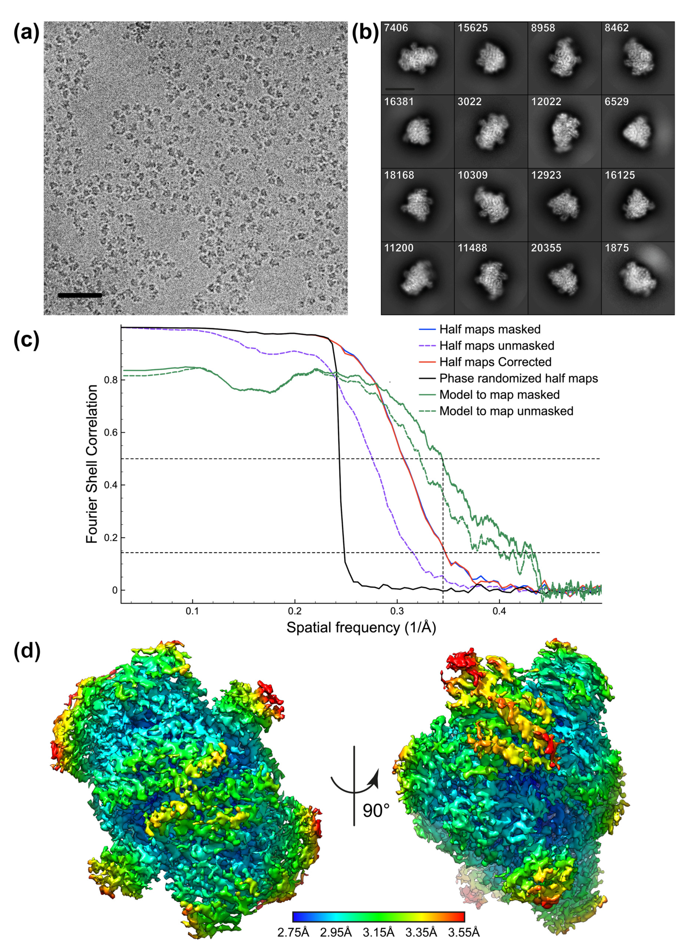
3.2.2. PFOR
4. Discussion
5. Conclusions
Supplementary Materials
Author Contributions
Funding
Institutional Review Board Statement
Informed Consent Statement
Data Availability Statement
Acknowledgments
Conflicts of Interest
References
- Dupont, C.L.; Yang, S.; Palenik, B.; Bourne, P.E. Modern Proteomes Contain Putative Imprints of Ancient Shifts in Trace Metal Geochemistry. Proc. Natl. Acad. Sci. USA 2006, 103, 17822–17827. [Google Scholar] [CrossRef] [PubMed] [Green Version]
- Wächtershäuser, G. Before Enzymes and Templates: Theory of Surface Metabolism. Microbiol. Rev. 1988, 52, 452–484. [Google Scholar] [CrossRef] [PubMed]
- Maret, W. Metalloproteomics, Metalloproteomes, and the Annotation of Metalloproteins. Metallomics 2010, 2, 117–125. [Google Scholar] [CrossRef] [PubMed]
- Beinert, H.; Holm, R.H.; Münck, E. Iron-Sulfur Clusters: Nature’s Modular, Multipurpose Structures. Science 1997, 277, 653–659. [Google Scholar] [CrossRef] [PubMed]
- Fontecilla-Camps, J.C.; Amara, P.; Cavazza, C.; Nicolet, Y.; Volbeda, A. Structure-Function Relationships of Anaerobic Gas-Processing Metalloenzymes. Nature 2009, 460, 814–822. [Google Scholar] [CrossRef] [PubMed]
- Imlay, J.A. Iron-Sulphur Clusters and the Problem with Oxygen. Mol. Microbiol. 2006, 59, 1073–1082. [Google Scholar] [CrossRef] [PubMed]
- Nicolet, Y.; Fontecilla-Camps, J.C. Iron-Sulfur Clusters and Molecular Oxygen: Function, Adaptation, Degradation and Repair. In 10 Iron-Sulfur Clusters and Molecular Oxygen: Function, Adaptation, Degradation and Repair; De Gruyter: Berlin, Germany, 2014; pp. 239–266. ISBN 978-3-11-030842-6. [Google Scholar]
- Volbeda, A.; Charon, M.H.; Piras, C.; Hatchikian, E.C.; Frey, M.; Fontecilla-Camps, J.C. Crystal Structure of the Nickel-Iron Hydrogenase from Desulfovibrio Gigas. Nature 1995, 373, 580–587. [Google Scholar] [CrossRef] [PubMed]
- Dobbek, H.; Svetlitchnyi, V.; Gremer, L.; Huber, R.; Meyer, O. Crystal Structure of a Carbon Monoxide Dehydrogenase Reveals a [Ni-4Fe-5S] Cluster. Science 2001, 293, 1281–1285. [Google Scholar] [CrossRef] [PubMed] [Green Version]
- Schindelin, H.; Kisker, C.; Schlessman, J.L.; Howard, J.B.; Rees, D.C. Structure of ADP × AIF4(-)-Stabilized Nitrogenase Complex and Its Implications for Signal Transduction. Nature 1997, 387, 370–376. [Google Scholar] [CrossRef] [PubMed]
- Doukov, T.I.; Iverson, T.M.; Seravalli, J.; Ragsdale, S.W.; Drennan, C.L. A Ni-Fe-Cu Center in a Bifunctional Carbon Monoxide Dehydrogenase/ Acetyl-CoA Synthase. Science 2002, 298, 567–572. [Google Scholar] [CrossRef] [PubMed] [Green Version]
- Darnault, C.; Volbeda, A.; Kim, E.J.; Legrand, P.; Vernède, X.; Lindahl, P.A.; Fontecilla-Camps, J.C. Ni-Zn-[Fe4-S4] and Ni-Ni-[Fe4-S4] Clusters in Closed and Open Subunits of Acetyl-CoA Synthase/Carbon Monoxide Dehydrogenase. Nat. Struct. Biol. 2003, 10, 271–279. [Google Scholar] [CrossRef] [PubMed]
- Allegretti, M.; Mills, D.J.; McMullan, G.; Kühlbrandt, W.; Vonck, J. Atomic Model of the F420-Reducing [NiFe] Hydrogenase by Electron Cryo-Microscopy Using a Direct Electron Detector. elife 2014, 3, e01963. [Google Scholar] [CrossRef] [PubMed] [Green Version]
- Akiba, T.; Toyoshima, C.; Matsunaga, T.; Kawamoto, M.; Kubota, T.; Fukuyama, K.; Namba, K.; Matsubara, H. Three-Dimensional Structure of Bovine Cytochrome Bc1 Complex by Electron Cryomicroscopy and Helical Image Reconstruction. Nat. Struct. Biol. 1996, 3, 553–561. [Google Scholar] [CrossRef] [PubMed]
- Su, C.-C.; Lyu, M.; Morgan, C.E.; Bolla, J.R.; Robinson, C.V.; Yu, E.W. A ‘Build and Retrieve’ Methodology to Simultaneously Solve Cryo-EM Structures of Membrane Proteins. Nat. Methods 2021, 18, 69–75. [Google Scholar] [CrossRef] [PubMed]
- Parey, K.; Lasham, J.; Mills, D.J.; Djurabekova, A.; Haapanen, O.; Yoga, E.G.; Xie, H.; Kühlbrandt, W.; Sharma, V.; Vonck, J.; et al. High-Resolution Structure and Dynamics of Mitochondrial Complex I—Insights into the Proton Pumping Mechanism. Sci. Adv. 2021, 7, eabj3221. [Google Scholar] [CrossRef] [PubMed]
- Parey, K.; Haapanen, O.; Sharma, V.; Köfeler, H.; Züllig, T.; Prinz, S.; Siegmund, K.; Wittig, I.; Mills, D.J.; Vonck, J.; et al. High-Resolution Cryo-EM Structures of Respiratory Complex I: Mechanism, Assembly and Disease. Sci. Adv. 2019, 5, eaax9484. [Google Scholar] [CrossRef] [PubMed] [Green Version]
- Wenke, B.B. The Many Roles of the Nitrogenase Iron Protein; California Institute Of Technology: Pasadena, CA, USA, 2019. [Google Scholar]
- Cohen, S.E.; Brignole, E.J.; Wittenborn, E.C.; Can, M.; Thompson, S.; Ragsdale, S.W.; Drennan, C.L. Negative-Stain Electron Microscopy Reveals Dramatic Structural Rearrangements in Ni-Fe-S-Dependent Carbon Monoxide Dehydrogenase/Acetyl-CoA Synthase. Structure 2021, 29, 43–49.e3. [Google Scholar] [CrossRef] [PubMed]
- Vernède, X.; Fontecilla-Camps, J.C. A Method to Stabilize Reduced and/or Gas-Treated Protein Crystals by Flash-Cooling under a Controlled Atmosphere. J. Appl. Cryst. J. Appl. Crystallogr. 1999, 32, 505–509. [Google Scholar] [CrossRef]
- Martin, L.; Vernède, X.; Nicolet, Y. Methods to Screen for Radical SAM Enzyme Crystallization Conditions. Methods Mol. Biol. 2021, 2353, 333–348. [Google Scholar] [CrossRef]
- Gerl, M.; Jaenicke, R. Assembly of Apoferritin from Horse Spleen: Comparison of the Protein in Its Native and Reassembled State. Biol. Chem. Hoppe. Seyler. 1987, 368, 387–396. [Google Scholar] [CrossRef]
- Yip, K.M.; Fischer, N.; Paknia, E.; Chari, A.; Stark, H. Atomic-Resolution Protein Structure Determination by Cryo-EM. Nature 2020, 587, 157–161. [Google Scholar] [CrossRef] [PubMed]
- Kontziampasis, D.; Klebl, D.P.; Iadanza, M.G.; Scarff, C.A.; Kopf, F.; Sobott, F.; Monteiro, D.C.F.; Trebbin, M.; Muench, S.P.; White, H.D. A Cryo-EM Grid Preparation Device for Time-Resolved Structural Studies. IUCrJ 2019, 6, 1024–1031. [Google Scholar] [CrossRef] [PubMed] [Green Version]
- Kerscher, L.; Oesterhelt, D. Pyruvate: Ferredoxin Oxidoreductase—New Findings on an Ancient Enzyme. Trends Biochem. Sci. 1982, 7, 371–374. [Google Scholar] [CrossRef]
- Chabrière, E.; Charon, M.H.; Volbeda, A.; Pieulle, L.; Hatchikian, E.C.; Fontecilla-Camps, J.C. Crystal Structures of the Key Anaerobic Enzyme Pyruvate:Ferredoxin Oxidoreductase, Free and in Complex with Pyruvate. Nat. Struct. Biol. 1999, 6, 182–190. [Google Scholar] [CrossRef] [PubMed]
- Chabrière, E.; Vernède, X.; Guigliarelli, B.; Charon, M.H.; Hatchikian, E.C.; Fontecilla-Camps, J.C. Crystal Structure of the Free Radical Intermediate of Pyruvate:Ferredoxin Oxidoreductase. Science 2001, 294, 2559–2563. [Google Scholar] [CrossRef] [PubMed]
- Cavazza, C.; Contreras-Martel, C.; Pieulle, L.; Chabrière, E.; Hatchikian, E.C.; Fontecilla-Camps, J.C. Flexibility of Thiamine Diphosphate Revealed by Kinetic Crystallographic Studies of the Reaction of Pyruvate-Ferredoxin Oxidoreductase with Pyruvate. Structure 2006, 14, 217–224. [Google Scholar] [CrossRef] [PubMed]
- Pieulle, L.; Guigliarelli, B.; Asso, M.; Dole, F.; Bernadac, A.; Hatchikian, E.C. Isolation and Characterization of the Pyruvate-Ferredoxin Oxidoreductase from the Sulfate-Reducing Bacterium Desulfovibrio Africanus. Biochim. Biophys. Acta. 1995, 1250, 49–59. [Google Scholar] [CrossRef]
- MacFarlane, D.R.; Angell, C.A. Glass Transition for Amorphous Solid Water. J. Phys. Chem. 1984, 88, 759–762. [Google Scholar] [CrossRef]
- Schorb, M.; Haberbosch, I.; Hagen, W.J.H.; Schwab, Y.; Mastronarde, D.N. Software Tools for Automated Transmission Electron Microscopy. Nat. Methods 2019, 16, 471–477. [Google Scholar] [CrossRef] [PubMed]
- Zivanov, J.; Nakane, T.; Forsberg, B.O.; Kimanius, D.; Hagen, W.J.; Lindahl, E.; Scheres, S.H. New Tools for Automated High-Resolution Cryo-EM Structure Determination in RELION-3. elife 2018, 7, e42166. [Google Scholar] [CrossRef]
- Zheng, S.Q.; Palovcak, E.; Armache, J.-P.; Verba, K.A.; Cheng, Y.; Agard, D.A. MotionCor2: Anisotropic Correction of Beam-Induced Motion for Improved Cryo-Electron Microscopy. Nat. Methods 2017, 14, 331–332. [Google Scholar] [CrossRef] [PubMed] [Green Version]
- Rohou, A.; Grigorieff, N. CTFFIND4: Fast and Accurate Defocus Estimation from Electron Micrographs. J. Struct. Biol. 2015, 192, 216–221. [Google Scholar] [CrossRef] [PubMed]
- Kucukelbir, A.; Sigworth, F.J.; Tagare, H.D. Quantifying the Local Resolution of Cryo-EM Density Maps. Nat. Methods 2014, 11, 63–65. [Google Scholar] [CrossRef] [PubMed] [Green Version]
- Pettersen, E.F.; Goddard, T.D.; Huang, C.C.; Couch, G.S.; Greenblatt, D.M.; Meng, E.C.; Ferrin, T.E. UCSF Chimera—A Visualization System for Exploratory Research and Analysis. J. Compu. Chem. 2004, 25, 1605–1612. [Google Scholar] [CrossRef] [PubMed] [Green Version]
- Pymol. The PyMOL Molecular Graphics System, Version 2.0 Schrödinger; DeLano Scientific LLC.: South San Francisco, CA, USA, 2021. [Google Scholar]
- Russo, C.J.; Passmore, L.A. Electron Microscopy: Ultrastable Gold Substrates for Electron Cryomicroscopy. Science 2014, 346, 1377–1380. [Google Scholar] [CrossRef] [PubMed] [Green Version]
- Emsley, P.; Lohkamp, B.; Scott, W.G.; Cowtan, K. Features and Development of Coot. Acta Cryst. 2010, 66, 486–501. [Google Scholar] [CrossRef] [PubMed] [Green Version]
- Afonine, P.V.; Poon, B.K.; Read, R.J.; Sobolev, O.V.; Terwilliger, T.C.; Urzhumtsev, A.; Adams, P.D. Real-Space Refinement in PHENIX for Cryo-EM and Crystallography. Acta Cryst. 2018, 74, 531–544. [Google Scholar] [CrossRef] [PubMed] [Green Version]
- Liebschner, D.; Afonine, P.V.; Baker, M.L.; Bunkóczi, G.; Chen, V.B.; Croll, T.I.; Hintze, B.; Hung, L.-W.; Jain, S.; McCoy, A.J.; et al. Macromolecular Structure Determination Using X-rays, Neutrons and Electrons: Recent Developments in Phenix. Acta Cryst. 2019, 75, 861–877. [Google Scholar] [CrossRef] [PubMed] [Green Version]
- Mikhal’chenko, R.S.; Getmanets, V.F.; Arkhipov, V.T. Peculiarities of Heat Transfer in Porous Solid Nitrogen. J. Eng. Phys. 1972, 23, 1075–1081. [Google Scholar] [CrossRef]
- Velikov, V.; Borick, S.; Angell, C.A. The Glass Transition of Water, Based on Hyperquenching Experiments. Science 2001, 294, 2335–2338. [Google Scholar] [CrossRef] [PubMed]
- Dobro, M.J.; Melanson, L.A.; Jensen, G.J.; McDowall, A.W. Chapter Three-Plunge Freezing for Electron Cryomicroscopy. In Methods in Enzymology; Jensen, G.J., Ed.; Cryo-EM Part A Sample Preparation and Data Collection; Academic Press: Cambridge, MA, USA, 2010; Volume 481, pp. 63–82. [Google Scholar]
- Nakane, T.; Kotecha, A.; Sente, A.; McMullan, G.; Masiulis, S.; Brown, P.M.G.E.; Grigoras, I.T.; Malinauskaite, L.; Malinauskas, T.; Miehling, J.; et al. Single-Particle Cryo-EM at Atomic Resolution. Nature 2020, 587, 152–156. [Google Scholar] [CrossRef] [PubMed]
- Chen, P.Y.-T.; Aman, H.; Can, M.; Ragsdale, S.W.; Drennan, C.L. Binding Site for Coenzyme A Revealed in the Structure of Pyruvate:Ferredoxin Oxidoreductase from Moorella Thermoacetica. Proc. Natl. Acad. Sci. USA 2018, 115, 3846–3851. [Google Scholar] [CrossRef] [PubMed] [Green Version]
- Vita, N.; Hatchikian, E.C.; Nouailler, M.; Dolla, A.; Pieulle, L. Disulfide Bond-Dependent Mechanism of Protection against Oxidative Stress in Pyruvate-Ferredoxin Oxidoreductase of Anaerobic Desulfovibrio Bacteria. Biochemistry 2008, 47, 957–964. [Google Scholar] [CrossRef] [PubMed]
- Senda, M.; Senda, T. Anaerobic Crystallization of Proteins. Biophys. Rev. 2017, 10, 183–189. [Google Scholar] [CrossRef] [PubMed] [Green Version]
- Jacobsen, R.T.; Stewart, R.B.; Jahangiri, M. A Thermodynamic Property Formulation for Nitrogen from the Freezing Line to 2000 K at Pressures to 1000 MPa. Int. J. 1986, 7, 503–511. [Google Scholar] [CrossRef]
- Engineering ToolBox Nitrogen-Thermophysical Properties. Available online: https://www.engineeringtoolbox.com/nitrogen-d_1421.html (accessed on 12 January 2021).


| Apoferritin (EMD-13487) | PFOR (EMD-13493) | |
|---|---|---|
| Magnification | 45,000 | 45,000 |
| Voltage (kV) | 200 | 200 |
| Total electron exposure (e−/Å2) | 60 | 60 |
| Defocus range (µm) | −0.9 to −2.55 | −0.5 to −3.5 |
| Pixel size (Å) | 0.899 | 0.899 |
| Symmetry imposed | Octahedral | C2 |
| Number of movies | 961 | 1304 |
| Number of particles images in the final map | 66,655 | 180,868 |
| Map resolution (Å) | 2.40 | 2.90 |
| FSC threshold | 0.143 | 0.143 |
| Apoferritin | PFOR (PDB-7PLM) | |
|---|---|---|
| Initial model used (PDB code) | 4V1W | 1B0P |
| Model resolution (Å) | 2.40 | 2.31 |
| Map sharpening B factor (Å2) | −118 | −91.7 |
| Model composition | ||
| Chains | 24 | 2 |
| Protein residues | 4 008 | 2 354 |
| Water | 321 | 114 |
| Ligands | 0 | [Fe4S4] (6); Ca2+ (2); Mg2+ (2); TPP (2) |
| Average B factor (Å2) | ||
| Protein | 21.48 | 32.63 |
| Ligand | / | 20.48 |
| Water | 21.48 | 17.91 |
| R.m.s. deviation | ||
| Bond lengths (Å) | 0.006 | 0.006 |
| Bond angles (°) | 0.952 | 0.691 |
| Validation | ||
| MolProbity score | 1.22 | 2.50 |
| Clash score | 4.45 | 13.90 |
| Rotamer outliers (%) | 0.00 | 4.98 |
| Ramachandran plot | ||
| Favored (%) | 99.34 | 95.47 |
| Allowed (%) | 0.66 | 4.53 |
| Disallowed (%) | 0.00 | 0.00 |
| Model vs. Data | ||
| CC (mask) | 0.88 | 0.76 |
| CC (main chain) | 0.87 | 0.75 |
| Mean CC for ligands | 0.77 | 0.62 |
Publisher’s Note: MDPI stays neutral with regard to jurisdictional claims in published maps and institutional affiliations. |
© 2022 by the authors. Licensee MDPI, Basel, Switzerland. This article is an open access article distributed under the terms and conditions of the Creative Commons Attribution (CC BY) license (https://creativecommons.org/licenses/by/4.0/).
Share and Cite
Cherrier, M.V.; Vernède, X.; Fenel, D.; Martin, L.; Arragain, B.; Neumann, E.; Fontecilla-Camps, J.C.; Schoehn, G.; Nicolet, Y. Oxygen-Sensitive Metalloprotein Structure Determination by Cryo-Electron Microscopy. Biomolecules 2022, 12, 441. https://doi.org/10.3390/biom12030441
Cherrier MV, Vernède X, Fenel D, Martin L, Arragain B, Neumann E, Fontecilla-Camps JC, Schoehn G, Nicolet Y. Oxygen-Sensitive Metalloprotein Structure Determination by Cryo-Electron Microscopy. Biomolecules. 2022; 12(3):441. https://doi.org/10.3390/biom12030441
Chicago/Turabian StyleCherrier, Mickaël V., Xavier Vernède, Daphna Fenel, Lydie Martin, Benoit Arragain, Emmanuelle Neumann, Juan C. Fontecilla-Camps, Guy Schoehn, and Yvain Nicolet. 2022. "Oxygen-Sensitive Metalloprotein Structure Determination by Cryo-Electron Microscopy" Biomolecules 12, no. 3: 441. https://doi.org/10.3390/biom12030441