
A Novel Longitudinal Phenotype–Genotype Association Study Based on Deep Feature Extraction and Hypergraph Models for Alzheimer’s Disease
 , ,
, ,
Abstract
:1. Introduction
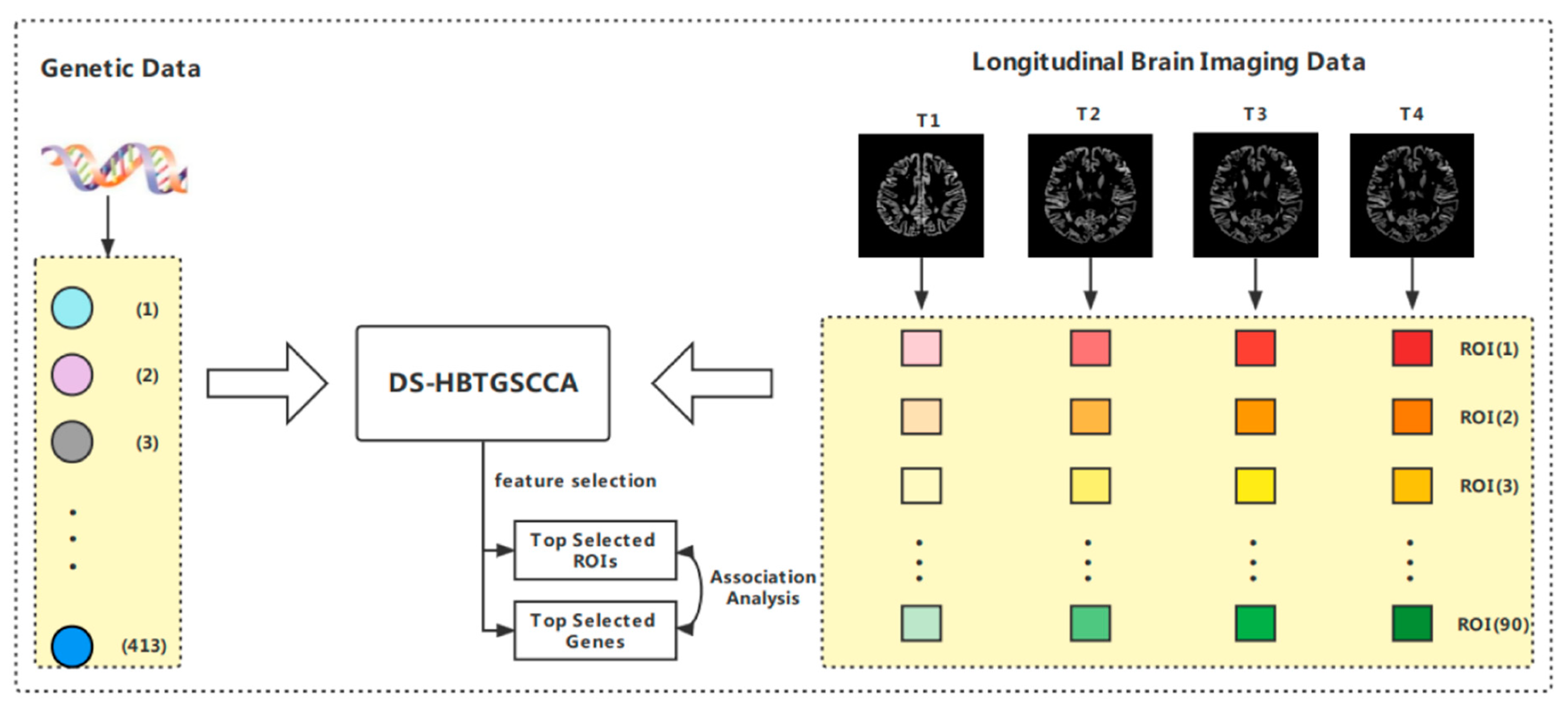
2. Methods
2.1. Data Source and Preprocessing
2.1.1. Preprocessing of Longitudinal Imaging Data
2.1.2. Preprocessing of Gene Expression Data
2.2. Deep Subspace Reconstruction Algorithm
2.3. Hypergraph Learning
2.4. The Proposed Optimization Algorithm
2.5. Performance Index of the Algorithm
2.6. Regression Index
2.7. Statistical Analysis
3. Results
3.1. On Simulation Data
3.2. On Real Imaging Genetic Data
3.3. Top ROIs and Top Genes Identification
3.4. Regression Results Using Selected Top Markers
3.5. Effectiveness Verification Results of Deep Subspace Reconstruction
4. Discussion
4.1. Biological Significance Analysis of Top ROIs
4.2. Correlation Analysis between Time-Series Related ROIs and Top Genes
4.3. Biological Significance Analysis of Top Genes
4.4. Regression Analysis
5. Conclusions
Supplementary Materials
Author Contributions
Funding
Institutional Review Board Statement
Informed Consent Statement
Data Availability Statement
Acknowledgments
Conflicts of Interest
References
- Thies, W.; Bleiler, L. Alzheimer’s Association 2013 Alzheimer’s disease facts and figures. Alzheimer’s Dement. 2013, 9, 208–245. [Google Scholar] [CrossRef]
- Kumar, A.; Sidhu, J.; Goyal, A.; Tsao, J.W. Alzheimer Disease; StatPearls Publishing: Treasure Island, FL, USA, 2022. [Google Scholar]
- Cheng, B.; Liu, M.; Zhang, D.; Shen, D. Robust multi-label transfer feature learning for early diagnosis of Alzheimer’s disease. Brain Imaging Behav. 2019, 13, 138–153. [Google Scholar] [CrossRef] [PubMed]
- Du, L.; Liu, K.; Zhu, L.; Yao, X.; Risacher, S.L.; Guo, L.; Saykin, A.J.; Shen, L. Identifying progressive imaging genetic patterns via multi-task sparse canonical correlation analysis: A longitu-dinal study of the ADNI cohort. Bioinformatics 2019, 35, i474–i483. [Google Scholar] [CrossRef]
- Huang, M.; Chen, X.; Yu, Y.; Lai, H.; Feng, Q. Imaging Genetics Study Based on a Temporal Group Sparse Regression and Additive Model for Biomarker Detection of Alzheimer’s Disease. IEEE Trans. Med. Imaging 2021, 40, 1461–1473. [Google Scholar] [CrossRef]
- Huang, M.; Yu, Y.; Yang, W.; Feng, Q.; Alzheimer’s Disease Neuroimaging Initiative. Incorporating spatial–anatomical similarity into the VGWAS framework for AD biomarker detection. Bioinformatics 2019, 35, 5271–5280. [Google Scholar] [CrossRef] [PubMed]
- Witten, D.M.; Tibshirani, R.J. Extensions of Sparse Canonical Correlation Analysis with Applications to Genomic Data. Stat. Appl. Genet. Mol. Biol. 2009, 8, 1–27. [Google Scholar] [CrossRef] [PubMed]
- Hotelling, H. Relations between two sets of variates. Biometrika 1936, 28, 321–377. [Google Scholar] [CrossRef]
- Fang, J.; Lin, D.; Schulz, S.C.; Xu, Z.; Calhoun, V.D.; Wang, Y.-P. Joint sparse canonical correlation analysis for detecting differential imaging genetics modules. Bioinformatics 2016, 32, 3480–3488. [Google Scholar] [CrossRef]
- Kim, M.; Won, J.H.; Youn, J.; Park, H. Joint-Connectivity-Based Sparse Canonical Correlation Analysis of Imaging Genetics for Detecting Biomarkers of Parkinson’s Disease. IEEE Trans. Med. Imaging 2020, 39, 23–34. [Google Scholar] [CrossRef] [PubMed]
- Wang, X.; Chen, H.; Yan, J.; Nho, K.; Risacher, S.L.; Saykin, A.J.; Shen, L.; Huang, H.; Adni, F.T. Quantitative trait loci identification for brain endophenotypes via new additive model with random networks. Bioinformatics 2018, 34, i866–i874. [Google Scholar] [CrossRef] [PubMed]
- Hao, X.; Li, C.; Yan, J.; Yao, X.; Risacher, S.L.; Saykin, A.J.; Shen, L.; Zhang, D.; Alzheimer’s Disease Neuroimaging Initiative. Identification of associations between genotypes and longitudinal phenotypes via temporally-constrained group sparse canonical correlation analysis. Bioinformatics 2017, 33, i341–i349. [Google Scholar] [CrossRef]
- Brand, L.; Nichols, K.; Wang, H.; Shen, L.; Huang, H. Joint Multi-Modal Longitudinal Regression and Classification for Alzheimer’s Disease Prediction. IEEE Trans. Med. Imaging 2020, 39, 1845–1855. [Google Scholar] [CrossRef] [PubMed]
- Murray, S.J. Apprendre R en un Jour. 2017. Available online: https://www.amazon.com/dp/B071W6ZJCV/ref=sr_1_1?s=digital-text&ie=UTF8&qid=1496261881&sr=1-1 (accessed on 30 May 2017).
- Wang, M.; Shao, W.; Hao, X.; Zhang, D. Identify Complex Imaging Genetic Patterns via Fusion Self-Expressive Network Analysis. IEEE Trans. Med. Imaging 2021, 40, 1673–1686. [Google Scholar] [CrossRef]
- Wang, M.; Shao, W.; Hao, X.; Huang, S.; Zhang, D. Identify connectome between genotypes and brain network phenotypes via deep self-reconstruction sparse canonical correlation analysis. Bioinformatics 2022, 38, 2323–2332. [Google Scholar] [CrossRef]
- Shao, W.; Peng, Y.; Zu, C.; Wang, M.; Zhang, D.; The Alzheimer’s Disease Neuroimaging Initiative. Hypergraph based multi-task feature selection for multimodal classification of Alzheimer’s disease. Comput. Med. Imaging Graph. 2020, 80, 101663. [Google Scholar] [CrossRef]
- Schölkopf, B.; Platt, J.; Hoffman, T. (Eds.) Learning with hypergraphs: Clustering, classification, and embedding. In Advances in Neural Information Processing Systems 19 (NIPS 2006); MIT Press: Cambridge, MA, USA, 2007; pp. 1601–1608. [Google Scholar]
- Liao, Z.; Zhao, X.; Li, T.; Mao, Y.; Hu, J.; Le, D.; Pei, Y.; Chen, Y.; Qiu, Y.; Zhu, J.; et al. EEG power spectral analysis reveals tandospirone improves anxiety symptoms in patients with Alzheimer’s disease: A prospective cohort study. Ann. Transl. Med. 2021, 9, 64. [Google Scholar] [CrossRef]
- Wang, X.; Cui, X.; Ding, C.; Li, D.; Cheng, C.; Wang, B.; Xiang, J. Deficit of Cross-Frequency Integration in Mild Cognitive Impairment and Alzheimer’s Disease: A Multilayer Network Approach. J. Magn. Reson. Imaging 2020, 53, 1387–1398. [Google Scholar] [CrossRef]
- Liu, L.; Jiang, H.; Wang, D.; Zhao, X.-F. A study of regional homogeneity of resting-state Functional Magnetic Resonance Imaging in mild cognitive impairment. Behav. Brain Res. 2021, 402, 113103. [Google Scholar] [CrossRef] [PubMed]
- Zhang, X.Y.; Wang, Y.F.; Zheng, L.J.; Zhang, H.; Lin, L.; Lu, G.M.; Zhang, L.J. Impacts of AD-Related ABCA7 and CLU Variants on Default Mode Network Connectivity in Healthy Middle-Age Adults. Front. Mol. Neurosci. 2020, 13, 145. [Google Scholar] [CrossRef]
- Sakurai, Y.; Mimura, I.; Mannen, T. Agraphia for Kanji Resulting from a Left Posterior Middle Temporal Gyrus Lesion. Behav. Neurol. 2008, 19, 93–106. [Google Scholar] [CrossRef]
- Visser, M.; Embleton, K.; Jefferies, E.; Parker, G.; Ralph, M.L. The inferior, anterior temporal lobes and semantic memory clarified: Novel evidence from distortion-corrected fMRI. Neuropsychologia 2010, 48, 1689–1696. [Google Scholar] [CrossRef]
- Kotloski, R.; Lynch, M.; Lauersdorf, S.; Sutula, T. Repeated brief seizures induce progressive hippocampal neuron loss and memory deficits. Prog. Brain Res. 2002, 135, 95–110. [Google Scholar] [CrossRef]
- Sass, K.J.; Spencer, D.D.; Kim, J.H.; Westerveld, M.; Novelly, R.A.; Lencz, T. Verbal memory impairment correlates with hippocampal pyramidal cell density. Neurology 1990, 40, 1694. [Google Scholar] [CrossRef]
- Reminger, S.L.; Kaszniak, A.W.; Labiner, D.M.; Littrell, L.D.; David, B.T.; Ryan, L.; Herring, A.M.; Kaemingk, K.L. Bilateral hippocampal volume predicts verbal memory function in temporal lobe epilepsy. Epilepsy Behav. 2004, 5, 687–695. [Google Scholar] [CrossRef]
- Sierksma, A.; Lu, A.; Mancuso, R.; Fattorelli, N.; Thrupp, N.; Salta, E.; Zoco, J.; Blum, D.; Buée, L.; De Strooper, B.; et al. Novel Alzheimer risk genes determine the microglia response to amyloid-β but not to TAU pathology. EMBO Mol. Med. 2020, 12, e10606. [Google Scholar] [CrossRef]
- Akiyama, H.; Barger, S.; Barnum, S.; Bradt, B.; Bauer, J.; Cole, G.M.; Cooper, N.R.; Eikelenboom, P.; Emmerling, M.; Fiebich, B.L.; et al. Inflammation and Alzheimer’s disease. Neurobiol. Aging 2000, 21, 383–421. [Google Scholar] [CrossRef]
- Bostancıklıoğlu, M. An update on the interactions between Alzheimer’s disease, autophagy and inflammation. Gene 2019, 705, 157–166. [Google Scholar] [CrossRef]
- Behl, C. Apoptosis and Alzheimer’s disease. J. Neural Transm. 2000, 107, 1325–1344. [Google Scholar] [CrossRef]
- Gaestel, M. What goes up must come down: Molecular basis of MAPKAP kinase 2/3-dependent regulation of the inflammatory response and its inhibition. Biol. Chem. 2013, 394, 1301–1315. [Google Scholar] [CrossRef]
- Sanfilippo, C.; Castrogiovanni, P.; Imbesi, R.; Di Rosa, M. CHI3L2 Expression Levels Are Correlated with AIF1, PECAM1, and CALB1 in the Brains of Alzheimer’s Disease Patients. J. Mol. Neurosci. 2020, 70, 1598–1610. [Google Scholar] [CrossRef]
- Son, S.M.; Nam, D.W.; Cha, M.-Y.; Kim, K.H.; Byun, J.; Ryu, H.; Mook-Jung, I. Thrombospondin-1 prevents amyloid beta–mediated synaptic pathology in Alzheimer’s disease. Neurobiol. Aging 2015, 36, 3214–3227. [Google Scholar] [CrossRef] [PubMed]
- Kim, D.H.; Lim, H.; Lee, D.; Choi, S.J.; Oh, W.; Yang, Y.S.; Oh, J.S.; Hwang, H.H.; Jeon, H.B. Thrombospondin-1 secreted by human umbilical cord blood-derived mesenchymal stem cells rescues neurons from synaptic dysfunction in Alzheimer’s disease model. Sci. Rep. 2018, 8, 354. [Google Scholar] [CrossRef]
- Dong, Y.; Lagarde, J.; Xicota, L.; Corne, H.; Chantran, Y.; Chaigneau, T.; Crestani, B.; Bottlaender, M.; Potier, M.-C.; Aucouturier, P.; et al. Neutrophil hyperactivation correlates with Alzheimer’s disease progression. Ann. Neurol. 2018, 83, 387–405. [Google Scholar] [CrossRef] [PubMed]
- Baik, S.H.; Cha, M.-Y.; Hyun, Y.-M.; Cho, H.; Hamza, B.; Kim, D.K.; Han, S.-H.; Choi, H.; Kim, K.H.; Moon, M.; et al. Migration of neutrophils targeting amyloid plaques in Alzheimer’s disease mouse model. Neurobiol. Aging 2014, 35, 1286–1292. [Google Scholar] [CrossRef]
- Altinoz, M.A.; Ozpinar, A. PPAR-δ and erucic acid in multiple sclerosis and Alzheimer’s Disease. Likely benefits in terms of immunity and metabolism. Int. Immunopharmacol. 2019, 69, 245–256. [Google Scholar] [CrossRef]
- Zenaro, E.; Pietronigro, E.; Della Bianca, V.; Piacentino, G.; Marongiu, L.; Budui, S.; Turano, E.; Rossi, B.; Angiari, S.; Dusi, S.; et al. Neutrophils promote Alzheimer’s disease–like pathology and cognitive decline via LFA-1 integrin. Nat. Med. 2015, 21, 880–886. [Google Scholar] [CrossRef]
- Stock, A.J.; Kasus-Jacobi, A.; Pereira, H.A. The role of neutrophil granule proteins in neuroinflammation and Alzheimer’s disease. J. Neuroinflammation 2018, 15, 240. [Google Scholar] [CrossRef]
- Kong, Y.; Liu, K.; Hua, T.; Zhang, C.; Sun, B.; Guan, Y. PET Imaging of Neutrophils Infiltration in Alzheimer’s Disease Transgenic Mice. Front. Neurol. 2020, 11, 523798. [Google Scholar] [CrossRef] [PubMed]
- Evin, Q.-X.L.V. Platelets and Alzheimer’s disease: Potential of APP as a biomarker. World J. Psychiatry 2012, 2, 102–113. [Google Scholar] [CrossRef]
- Henry, A.; Li, Q.-X.; Galatis, D.; Hesse, L.; Multhaup, G.; Beyreuther, K.; Masters, C.L.; Cappai, R. Inhibition of platelet activation by the Alzheimer’s disease amyloid precursor protein. Br. J. Haematol. 1998, 103, 402–415. [Google Scholar] [CrossRef]
- Davies, T.; Long, H.; Sgro, K.; Rathbun, W.; McMenamin, M.; Seetoo, K.; Tibbles, H.; Billingslea, A.; Fine, R.; Fishman, J.; et al. Activated Alzheimer Disease Platelets Retain More Beta Amyloid Precursor Protein. Neurobiol. Aging 1997, 18, 147–153. [Google Scholar] [CrossRef] [PubMed]
- Bostancıklıoğlu, M. Optogenetic stimulation of serotonin nuclei retrieve the lost memory in Alzheimer’s disease. J. Cell. Physiol. 2020, 235, 836–847. [Google Scholar] [CrossRef]
- Yang, L.; Yin, T.; Liu, Y.; Sun, J.; Zhou, Y.; Liu, J. Gold nanoparticle-capped mesoporous silica-based H2O2-responsive controlled release system for Alzheimer’s disease treatment. Acta Biomater. 2016, 46, 177–190. [Google Scholar] [CrossRef]
- Webers, A.; Heneka, M.T.; Gleeson, P.A. The role of innate immune responses and neuroinflammation in amyloid accumulation and progression of Alzheimer’s disease. Immunol. Cell Biol. 2020, 98, 28–41. [Google Scholar] [CrossRef] [PubMed]
- Butler, C.A.; Popescu, A.S.; Kitchener, E.J.A.; Allendorf, D.H.; Puigdellívol, M.; Brown, G.C. Microglial phagocytosis of neurons in neurodegeneration, and its regulation. J. Neurochem. 2021, 158, 621–639. [Google Scholar] [CrossRef] [PubMed]


| Groups | AD | EMCI | LMCI | HC |
|---|---|---|---|---|
| Number | 10 | 102 | 36 | 62 |
| Gender(M/F) | 6/4 | 55/47 | 18/18 | 34/28 |
| Age (mean ± std) | 79.65 ± 9.77 | 70.95 ± 7.07 | 73.40 ± 7.19 | 75.83 ± 5.83 |
| Algorithm | T1 | T2 | T3 | T4 |
|---|---|---|---|---|
| TGSCCA | 0.6881 | 0.6754 | 0.6905 | 0.6799 |
| DS-HBTGSCCA | 0.7169 | 0.6967 | 0.6884 | 0.665 |
| Algorithm | T1 | T2 | T3 | T4 |
|---|---|---|---|---|
| TGSCCA | 0.1037 | 0.1138 | 0.1509 | 0.1699 |
| DS-HBTGSCCA | 0.2186 | 0.185 | 0.2036 | 0.1271 |
| T1 | T2 | T3 | T4 | |||||
|---|---|---|---|---|---|---|---|---|
| ROI | TGSCCA | DS-HBTGSCCA | TGSCCA | DS-HBTGSCCA | TGSCCA | DS-HBTGSCCA | TGSCCA | DS-HBTGSCCA |
| Left Middle Temporal | 0.242891 | 0.241756 | 0.24247 | 0.241756 | 0.241243 | 0.241756 | 0.240415 | 0.241756 |
| Right Middle Frontal | 0.239456 | 0.239911 | 0.239386 | 0.239911 | 0.240085 | 0.239911 | 0.240716 | 0.239911 |
| Right Middle Temporal | 0.239204 | 0.238587 | 0.239034 | 0.238587 | 0.238354 | 0.238587 | 0.237752 | 0.238587 |
| Left Middle Frontal | 0.231468 | 0.231956 | 0.231756 | 0.231956 | 0.23217 | 0.231956 | 0.232429 | 0.231956 |
| Right Inferior Temporal | 0.19458 | 0.193725 | 0.19405 | 0.193725 | 0.1936 | 0.193725 | 0.192668 | 0.193725 |
| Left Precuneus | 0.185073 | 0.185278 | 0.185006 | 0.185278 | 0.185381 | 0.185278 | 0.185652 | 0.185278 |
| Right Precuneus | 0.170217 | 0.170441 | 0.170298 | 0.170441 | 0.170519 | 0.170441 | 0.17073 | 0.170441 |
| Right Superior Frontal | 0.163554 | 0.163951 | 0.163448 | 0.163951 | 0.163973 | 0.163951 | 0.164824 | 0.163951 |
| Left Precentral | 0.156793 | 0.156955 | 0.156787 | 0.156955 | 0.157135 | 0.156955 | 0.157101 | 0.156955 |
| Right Postcentral | 0.154319 | 0.154576 | 0.154386 | 0.154576 | 0.154746 | 0.154576 | 0.154849 | 0.154576 |
| Gene | Weight |
|---|---|
| FCER1G | 0.02043 |
| AIF1.1 | 0.018494 |
| MORF4L1 | 0.018055 |
| PRR13 | 0.016633 |
| IL2RG | 0.015529 |
| EIF4EBP2.2 | 0.014426 |
| METTL9.1 | 0.014098 |
| PPT1.1 | 0.013179 |
| CCNY.2 | 0.013001 |
| TUBB1 | 0.012844 |
| MAPKAPK3.1 | 0.012789 |
| IER3 | 0.01205 |
| ATP6V1D.1 | 0.011843 |
| PECAM1 | 0.011714 |
| CELF2.1 | 0.011599 |
| PGAM1 || LOC643576 | 0.011451 |
| CORO1C.2 | 0.011208 |
| XRCC5 | 0.011188 |
| SUPT4H1.1 | 0.011082 |
| RTN4.1 | 0.010388 |
| ROI | Regression Method (Mean of R2_Score) | ||
|---|---|---|---|
| Bayes | LR | RD | |
| Left Middle Temporal | 0.953981 | 0.952863 | 0.801004 |
| Right Middle Frontal | 0.964647 | 0.958669 | 0.905144 |
| Right Middle Temporal | 0.970721 | 0.962353 | 0.956769 |
| Left Middle Frontal | 0.96607 | 0.945351 | 0.965932 |
| Right Inferior Temporal | 0.964978 | 0.932218 | 0.967617 |
| Left Precuneus | 0.972586 | 0.941337 | 0.974177 |
| Right Precuneus | 0.971747 | 0.940244 | 0.974972 |
| Right Superior Frontal | 0.967789 | 0.936142 | 0.977111 |
| Left Precentral | 0.968347 | 0.92251 | 0.977113 |
| Right Postcentral | 0.966746 | 0.907586 | 0.977428 |
| Contour Coefficient | F-Score | Precision | Recall | NMI | Adj-RI | ||
|---|---|---|---|---|---|---|---|
| Through multilayer neural network | Gene | 0.7675 | 0.4599 ± 0.0358 | 0.5267 ± 0.0486 | 0.4083 ± 0.0286 | 0.2747 ± 0.0514 | 0.2198 ± 0.0556 |
| T1 | 0.4667 | 0.3154 ± 0.0150 | 0.3610 ± 0.0045 | 0.2810 ± 0.0259 | 0.0259 ± 0.0043 | 0.0117 ± 0.0062 | |
| T2 | 0.5052 | 0.3655 ± 0.0289 | 0.3983 ± 0.0107 | 0.3391 ± 0.0417 | 0.0374 ± 0.0032 | 0.0642 ± 0.0190 | |
| T3 | 0.4723 | 0.2941 ± 0.0050 | 0.3532 ± 0.0035 | 0.2519 ± 0.0059 | 0.0198 ± 0.0060 | 0.0019 ± 0.0042 | |
| T4 | 0.4732 | 0.3462 ± 0.0088 | 0.3403 ± 0.0040 | 0.3529 ± 0.0190 | 0.0377 ± 0.0107 | 0.0181 ± 0.0070 | |
| Without multilayer neural network | Gene | 0.2478 | 0.3615 ± 0.0104 | 0.3709 ± 0.0056 | 0.3535 ± 0.0107 | 0.0786 ± 0.0073 | 0.0282 ± 0.0059 |
| T1 | 0.4731 | 0.3130 ± 0.0117 | 0.3552 ± 0.0037 | 0.2801 ± 0.0171 | 0.0142 ± 0.0060 | 0.0046 ± 0.0048 | |
| T2 | 0.4544 | 0.3087 ± 0.0061 | 0.3416 ± 0.0016 | 0.2817 ± 0.0097 | 0.0225 ± 0.0048 | 0.0133 ± 0.0022 | |
| T3 | 0.4414 | 0.3233 ± 0.0138 | 0.3594 ± 0.0077 | 0.2977 ± 0.0485 | 0.0354 ± 0.0106 | 0.0089 ± 0.0114 | |
| T4 | 0.4242 | 0.3022 ± 0.0068 | 0.3536 ± 0.0047 | 0.2641 ± 0.0098 | 0.0127 ± 0.0062 | 0.0023 ± 0.0056 | |
Disclaimer/Publisher’s Note: The statements, opinions and data contained in all publications are solely those of the individual author(s) and contributor(s) and not of MDPI and/or the editor(s). MDPI and/or the editor(s) disclaim responsibility for any injury to people or property resulting from any ideas, methods, instructions or products referred to in the content. |
© 2023 by the authors. Licensee MDPI, Basel, Switzerland. This article is an open access article distributed under the terms and conditions of the Creative Commons Attribution (CC BY) license (https://creativecommons.org/licenses/by/4.0/).
Share and Cite
Kong, W.; Xu, Y.; Wang, S.; Wei, K.; Wen, G.; Yu, Y.; Zhu, Y. A Novel Longitudinal Phenotype–Genotype Association Study Based on Deep Feature Extraction and Hypergraph Models for Alzheimer’s Disease. Biomolecules 2023, 13, 728. https://doi.org/10.3390/biom13050728
Kong W, Xu Y, Wang S, Wei K, Wen G, Yu Y, Zhu Y. A Novel Longitudinal Phenotype–Genotype Association Study Based on Deep Feature Extraction and Hypergraph Models for Alzheimer’s Disease. Biomolecules. 2023; 13(5):728. https://doi.org/10.3390/biom13050728
Chicago/Turabian StyleKong, Wei, Yufang Xu, Shuaiqun Wang, Kai Wei, Gen Wen, Yaling Yu, and Yuemin Zhu. 2023. "A Novel Longitudinal Phenotype–Genotype Association Study Based on Deep Feature Extraction and Hypergraph Models for Alzheimer’s Disease" Biomolecules 13, no. 5: 728. https://doi.org/10.3390/biom13050728