1. Introduction
Mobile ground robots are widely used for various tasks in indoor environments. The addition of multiple mobile ground robots is introduced to improve the efficiency of certain tasks, thus creating a multi-robot system. This paper introduces a multi-robot system that is collaborative and autonomous, where each robot has its own local task or goal, but the robots collaborate on global tasks such as mapping. This paper develops a movement algorithm for a multi-robot system with the ability to avoid obstacles while maintaining movement stability.
The motion of a mobile robot is based on the forward kinematics and the inverse kinematics. The kinematics models are needed to control the linear and angular velocities in order to complete the control task for the mobile robot [
1]. Extensive research has been conducted in the field of autonomous mobile robot navigation [
2,
3,
4,
5]. Navigation is a complex task and involves various techniques to gather and decode information. There are several adequate path planning algorithms that have been developed for mobile robot systems [
6]. This paper implemented the A* path planner because it considers the lowest cost per iteration move to be taken [
7]. A* determines the closest possible path from starting position to the goal point, making this an optimal search algorithm. Moreover, A* solves a given problem by evaluating all possible paths to determine the path that leads to the goal point fastest.
Previously developed motion control algorithms allow a mobile robot to avoid static and dynamic obstacles [
8,
9], while navigating in an indoor environment. Obstacle avoidance algorithms, such as the potential field method [
10,
11,
12], have been widely used. The concept of this method is to fill the workspace of the robot with an artificial potential field in which the robot is attracted towards the goal and repulsed away from the obstacles. Previously, this method was used to plan a path for a mobile robot in static environments [
13], but it has several shortcomings, such as the inability to reach a goal when it is near an obstacle. Moreover, the robot cannot navigate through a narrow line of obstacles due to the large repulsive field generated. Further drawbacks include motion oscillations near obstacles and local minima. However, in many implementations, the environment is dynamic and thus this method is not considered by the paper. Another popular obstacle avoidance algorithm is fuzzy control [
14,
15]. However, it has poor system control accuracy and, due to the algorithm lacking systematicity, the control goal cannot be defined. Model predictive control [
16,
17] is effectively used to overcome the trajectory tracking problem since it reduces the tracking error along the desired trajectory. Model predictive control predicts upcoming disturbances and plans upcoming actions accordingly. The algorithm improves the steady-state response which reduces the offset error and increases control accuracy.
This paper considers the virtual impedance algorithm for obstacle avoidance and local motion control in a multi-robot dynamic environment. Impedance control is used in dynamic environments because it relates the force and the position. The impedance control algorithm aims to set the dynamics of the system to a desired impedance defined by the user. This is the main difference since impedance control is used with an external force feedback [
18]. A repulsive force is generated from the obstacles, pushing the mobile ground robot away from the obstacles, but also away from the goal. The method compensates for the repulsive force by generating an attractive force towards the goal. The attractive and repulsive forces act as a spring and damper with the parameters, K and D, to define the strength of the forces. The total force acting on the mobile ground robot is the sum of the attractive and repulsive forces.
The traditional virtual impedance algorithm only generates an attractive force towards the goal and a situation could occur whereby the attractive force and repulsive forces are equal [
19]. Moreover, traditional virtual impedance control is susceptible to cause movement instability and oscillations near obstacles. This paper proposes a two-layered navigation strategy that incorporates a global path planner [
20], together with an improved adaptive virtual impedance algorithm to overcome these problems. The main contribution of this paper is the improvement in motion behaviour and movement stability of a multi-robot system navigating in a dynamic indoor environment.
This paper is organised as follows:
Section 2 describes the traditional virtual impedance control algorithm.
Section 3 introduces the new improved adaptive virtual impedance control method.
Section 4 defines the mathematical equations used in the model-based control strategy.
Section 5 describes the parameters of the adaptation algorithm used to improve the movement behaviour of a mobile multi-robot system.
Section 6 presents the simulated results together with real-world results obtained from experiments.
Section 7 concludes the paper and presents the perspectives of the work.
2. Virtual Impedance Control in a Multi-Robot Environment
The virtual impedance method considers a mobile robot moving in a multi-robot environment to be submitted to the following forces:
A repulsive force between the mobile robot and both the obstacles and the other mobile robots;
An attractive force between the mobile robot and the reference trajectory.
Leading to different types of interactions:
Interactions between robots;
Interactions between robots and obstacles;
Interactions between robots and reference trajectories.
Figure 1 shows the different interactions of a system with two mobile robots.
Each interaction is defined by a couple of parameters, K and D, representing the stiffness and the damping of the corresponding force [
21]. The dynamic behaviour of a robot
in a multi-robot environment is given by [
22]:
with
= 1…nb and nb the number of robots.
where:
: represents the attractive forces between the robot and its reference trajectory.
: concerns the repulsive forces between the robot and the objects in its vicinity, including fixed and dynamic objects.
is given by:
with
and
where:
: the virtual mass of the mobile robot.
: the current x position of the mobile robot.
: the desired x position of the reference trajectory.
K: stiffness tuning parameter.
D: damping tuning parameter.
: set of parameters defining the sensing envelope of the mobile robot.
The expressions of and show that a robot is taken into account only if it is in the interaction zone of the robot defined by .
Moreover, the interactions of the robot
with the obstacles are computed based on the information issued from the sensors (ultrasonic, IR or LiDAR) with which the robot is equipped, given that the environment is supposed to be unknown and dynamic. The update of the robot trajectory is based on the integration of Equation (1) with each sampling time. The movement of the robot at its next position is only allowed if it respects the avoiding security constraint [
19] given by:
Figure 2 illustrates the interactions between robot
and an obstacle, as well as the virtual sensing envelope.
Where is the distance between the robot and the obstacle, static or dynamic, and is the security distance defined within the virtual sensing envelope.
The development of the multi-robot system with the two-layered navigation strategy is based on the block diagram shown in
Figure 3.
Simultaneous localisation and mapping (SLAM) is used to build a map of the environment with the data received from the sensors [
23]. The global path planner uses the newly created map for trajectory planning. The entire block diagram is duplicated for a second, third or fourth robot added to the environment.
The kinematic model shown in
Figure 4, takes the velocity of the mobile robot and transforms it into the generalised coordinate vector by the following equation [
24]:
The velocity of the mobile robot can then be taken from each wheel velocity. The linear velocity of the mobile robot is expressed as:
The angular velocity of the mobile robot is expressed as:
where:
left wheel and right wheel velocity, respectively.
relative position of the mobile robot in inertia frame.
θ: relative heading of the mobile robot in inertia frame.
distance between left and right wheel.
radius of wheel.
: mobile robot’s centre linear velocity in a global reference frame from the two differential driving wheels.
: mobile robot’s centre angular velocity in a global reference frame from the two differential driving wheels.
The multi-robot system with the virtual impedance controller is represented in the block diagram in
Figure 5.
With this two-layered navigation strategy, the robot generates an attractive force towards the planned trajectory until the goal is reached. The attractive force is stable because the global trajectory planner plans an obstacle-free path from the starting position. The robot only generates a repulsive force if an obstacle (static or dynamic) enters into its security zone (defined within the sensing envelope). This is different from the potential field method that generates a repulsive force from an obstacle, no matter the position of the mobile robot. These forces can be controlled with the damping and stiffness parameters in order to find a good balance so that the robot will always avoid obstacles, yet remain attracted to the planned trajectory. However, the orientation of the robot becomes unstable as the robot reacts to the repulsive forces whilst being attracted to the reference trajectory. The oscillations are highlighted when the robot is subjected to multiple repulsive forces generated from multiple obstacles (static or dynamic).
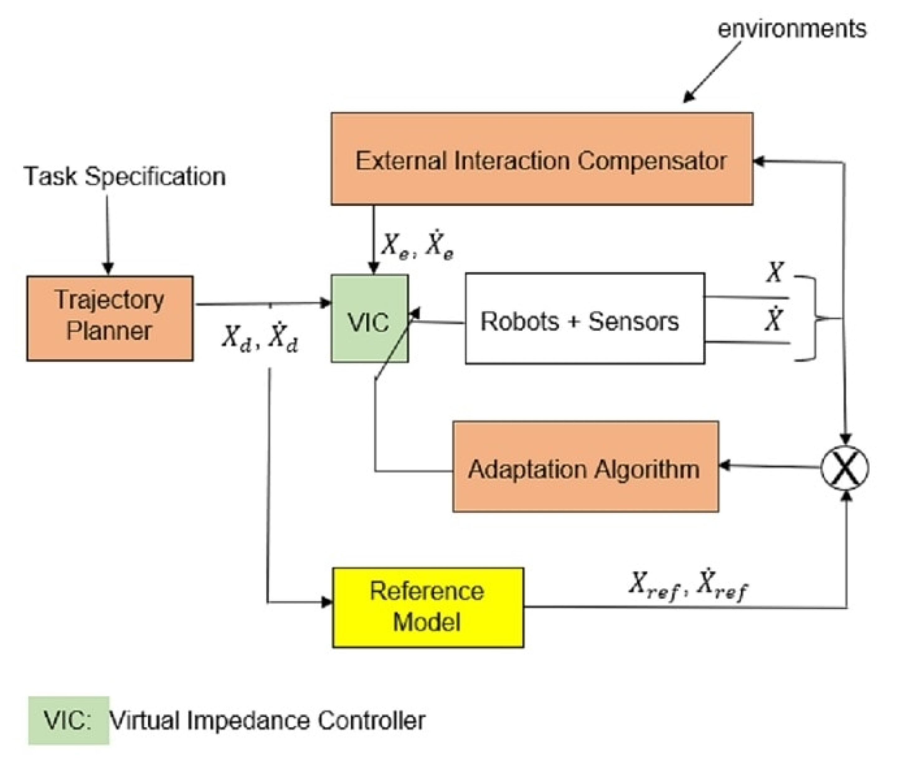
3. Improved Adaptive Virtual Impedance Control
A new adaptive virtual impedance method is proposed in
Figure 6 to overcome the instability problem of the conventional virtual impedance method. The improved control method aims to remove the orientation oscillations that occur when the mobile robot approaches obstacles.
The virtual impedance controller is modified by adding an adaptation algorithm and reference model for stable dynamic behaviour [
25,
26,
27]. The dynamic behaviour of the robot is given by the following equation:
with
: the robot position vector.
: the trajectory position vector.
: the obstacle position vector in the environment.
In state space form, the dynamic equation is written as follows:
with
and
represent the input vectors to the system.
The matrix is added when another mobile robot is added to the environment. Additional mobile robots can be added by adding more matrices. The current position of the robot, positions of obstacles and the position of the desired trajectory are used to formulate Equations (10) and (11). Next, we will look at the same system, but with two degrees of freedom (dof).
The extension of a system with two dof is defined using the new state vector
given by:
and
represent the input vectors of the system, with:
The new state space equation is given by:
with
and where
is a 2 × 2 zero matrix.
The 2 × 2 zero matrix is added because it represents the linear transformation, which transforms all the vectors to the zero vector. Equation (17) uses both the x and y positions and the matrices used are 4 × 4. The damping and stiffness parameters, K and D, can be tuned in the A and matrices to achieve different results. Increasing the K parameter will result in greater attractive and repulsive forces. The value of the damping parameter will influence the rate at which the robot recovers to the desired trajectory. A good balance between these parameters is required to achieve the desired motion behaviour.
The position and the speed of the robot are determined by the integration of Equation (17). The speed and acceleration are bounded by the actuators used on the physical robot in a real-world scenario.
4. Reference Model-Based Control Strategy
A reference model is defined in order to control the dynamic behaviour of the robot on its reference trajectory; this reference model is shown in the lower block in
Figure 6.
The reference model is defined by a second-order differential equation as follows:
If we defined the different state and control variables
Equation (11) is written in state space form as follows:
with
Now, we extend this representation to a system with two dof with
the state vector defined as follows:
The new state space equation is written as follows:
where:
with
and
given by:
The control architecture proposed in
Figure 6 shows that the system (robot and controller) is submitted to both the action of the environment (obstacles and other robots) that generates repulsive forces and to the attractive force generated by the error between the actual robot position and the desired position given by the desired trajectory. Each robot has the same control architecture. The parameters of the controller are adapted in real time such that each robot mimics the reference model [
28,
29].
The parameters, K and D, of each controller are adapted by the minimisation of the cost function defined, on one hand, by the quadratic error between the robot state vector with the reference model state vector and, on the other hand, by a constraint related in respect to a minimal security distance with the obstacles and with the other robots. The cost function is defined by:
where:
if and otherwise.
: a positive scalar used for the penalisation of the constraint related to the security distance.
: the security distance with respect to the distance between the robots.
: the distance between the robot and the robot ( = 1…nb and nb the number of robots. ( ≠ )).
: represents the boundary of the detection envelope of robot .
5. Parameters of Adaptation Algorithm
The adaptation of the parameters, K and D, implies the computation of the gradient of
, obtained as follows [
30], given that
The distance is defined as follows:
and
represent the state vectors of the robots
and
.
Combining Equations (28) and (29) leads to:
with
and
is obtained by the derivation of Equation (17), leading to:
For instance, by considering the parameters,
and
for the reference trajectory, Equation (34) is rewritten as follows:
with
, which are represented by the following matrices:
with
Let us define
The gradient method is used to compute the new parameter as follows:
Equation (42) is used to update the specific parameter chosen to represent .
6. Results
The results of the implemented adaptive virtual impedance control algorithm are presented below. The adaptive virtual impedance control algorithm forms part of the two-layered navigation strategy implemented by the paper. The global (higher) layer uses the A * path planner to plan a collision-free path to the goal using a pre-gathered grid map of the indoor environment. The local (lower) level uses the control algorithm for dynamic behaviour when avoiding the unknown static and dynamic obstacles that enter into the sensing envelope of the mobile robot.
The following simulation introduces an unknown obstacle (red block) into the environment. During the simulation, the robot makes use of its two-layered navigation strategy to plan a path and avoid obstacles during its navigation towards the goal. The motion behaviour and orientation oscillations when avoiding obstacles were closely observed.
At the start of navigation simulation 1, the implemented robot plans a collision-free path to the goal point using the A* path planner (
Figure 7a) unaware of the unknown obstacle (red block). The robot detects the obstacle 2m away, but the control algorithm only generates a repulsive force from the obstacle when it enters into the security zone (1 m), as seen in
Figure 7b. The movement of the robot experiences some instabilities due to the attractive and repulsive forces acting on it (
Figure 7c). The improved adaptive virtual impedance method generates an attractive force toward the planned trajectory instead of the goal point, this can clearly be seen in
Figure 7d. The robot returns to the desired trajectory that was planned at the start, instead of moving directly toward the goal. The A* star path planner does not re-plan a path during navigation. When an unknown obstacle enters the sensing envelope of the mobile robot, the generated repulsive force is far greater than the attractive force. This is to guarantee that the mobile robot avoids the obstacle. The parameters used during navigation simulation 1 are presented in
Table 1. The stable movement and motion behaviour of the mobile robot can be seen in the
Supplementary Material (Video S1).
Next, a real-world experiment was conducted. A similar floor layout was created by placing obstacles in similar positions to match those in the simulation. The reason for conducting the experiment was to test the adaptive virtual impedance algorithm in a real-world scenario. The same parameters were used during the real-world experiment.
The robot pre-plans a collision-free path to the goal in
Figure 8a. The robot detects the red obstacle in
Figure 8b and relies on the control algorithm to avoid the obstacle. The mobile robot avoided the red obstacle and returned to the planned path before moving to the goal (
Figure 8c). The path planned by the mobile can be seen in the
Supplementary Material (Video S2). The movement behaviour of the mobile robot when avoiding the red obstacle can be seen in the
Supplementary Material (Video S3).
The data on the graphs in
Figure 9 illustrate how the mobile robot reacts to detecting the unknown obstacle. The orientation of the mobile robot experiences minor oscillations, in both the simulation (
Figure 9a) and real world (
Figure 9b) when detecting the unknown obstacle. This is due to the avoidance algorithm of the robot, as it generates a repulsive force from the newly detected obstacle. The movement of the robot is improved from the conventional virtual impedance method and the results show a stable linear velocity with good motion behaviour.
The next experiment introduces a dynamic obstacle in the environment. The mobile robot plans a similar path from the starting position to the goal as in the previous simulation. The results of this simulation, in which the two-layered navigation strategy reacts to an unknown dynamic obstacle entering the sensing and security zone of the mobile robot, are presented below.
The implemented robot pre-plans a collision-free path to the goal in
Figure 10a. As the mobile robot moves along the desired trajectory in
Figure 10b, a dynamic obstacle moves in front of the mobile robot. The orientation of the robot experiences minor oscillations (
Figure 10c), as the algorithm generates a repulsive force from the newly detected dynamic obstacle. Since the obstacle is moving away from the mobile robot, the mobile robot recovers quickly and moves toward the goal point along the planned path (
Figure 10d). The reference model in the adaptive virtual impedance algorithm ensures that the desired behaviour in the transition phases is respected. The mobile robot moves back to the planned path as soon as the dynamic obstacle moves out of the security zone of the mobile robot and no longer obscures the path along the desired trajectory. The two-layered navigation strategy only makes use of the global path planner at the start of the simulation. The desired trajectory is not re-planned during the simulation. It is evident that the implemented robot took longer to return to the desired trajectory when a dynamic obstacle is in the close vicinity of the robot. The simulation tested the localisation, path planning and obstacle avoidance capabilities of the mobile robot in a dynamic environment. The parameters used during navigation simulation 2 are presented in
Table 2.
In
Figure 11a the mobile robot pre-plans a collision-free path to the goal. As the mobile robot approaches the goal, a human representing a dynamic obstacle, moves in front of the mobile robot (
Figure 11b). The dynamic obstacle continues to move away from the mobile robot in
Figure 11c. Once the dynamic obstacle moved away, the mobile robot was able to recover and reach the goal. The movement behaviour of the mobile robot when detecting and avoiding a dynamic obstacle can be seen in the
Supplementary Material (Video S4).
As seen in
Figure 12a, the angular velocity oscillates when a dynamic obstacle enters into the sensing envelope of the mobile robot. The angular velocity is volatile around the 14 s mark in
Figure 12b due to the presence of the dynamic obstacle as the robot tries to return to the planned path.
The following simulation implements multiple mobile robots. Each robot plans a path to its own goal point and uses the adaptive virtual impedance controller to avoid collisions.
The simulation in
Figure 13 implements multiple mobile robots. Each robot plans a path to its own goal point at the start (
Figure 13a) and uses the adaptive virtual impedance controller to avoid collisions (
Figure 13b). The simulation illustrated the avoidance capability of each mobile robot when their planned paths intersect (
Figure 13c). The result shows that the robots avoid collisions easier when the other dynamic obstacle detected is another mobile robot with the implemented two-layered navigation strategy (
Figure 13d). The result demonstrated that the mobile robots avoided a collision and each robot recovered to its own planned path. The mobile robots successfully implemented the two-layered navigation strategy in a dynamic multi-robot environment and maintained the desired behaviour with movement stability.
7. Conclusions and Future Work
The A* path planner successfully planned paths for single and multiple mobile robots in an environment with known and unknown obstacles. An optimal path with a desired trajectory toward the goal was generated for each mobile robot. It was noted that the A* path planner did not re-plan a new path once unknown obstacles were detected. This is a characteristic of the path planner that was welcomed, since the research aimed at developing a local motion control algorithm that would recover to the original path after avoiding an obstacle.
The conventional virtual impedance control method was improved to overcome drawbacks, such as severe oscillations in motion behaviour. The improved adaptive virtual impedance algorithm was implemented with the A* path planner in a two-layered navigation strategy. The obtained results show stable motion behaviour with good accuracy in environments with known obstacles. The introduction of a static unknown obstacle resulted in minor oscillations in motion behaviour. However, this had no effect on the travelled path and the motion remained smooth throughout. The mobile robot accurately recovered to the desired trajectory after avoiding the obstacle.
The motion behaviour of the mobile robot in a multi-robot dynamic environment experienced prolonged oscillations because of the unpredictability of dynamic obstacles. This can be reduced to a degree, by changing the stiffness and damping parameters. The system avoids local minima by applying the two-layered navigation strategy with the adaptive virtual impedance control method.
Real-world experiments were conducted using the TurtleBot 3 Burger. The obtained results validated the ones obtained in simulations. Successful experiments tested the two-layered navigation strategy with unknown and dynamic obstacles.
The autonomous collaborative robot system could have many different applications such as smart manufacturing or working in an environment with humans. Clinical arenas, such as hospitals and wellness centres, could benefit from collaborative mobile robotics. Such a robot system can aid in disinfecting areas, moving equipment, carrying medicine [
31], and even automate wheelchairs. The avoidance algorithm can be further developed to avoid dynamic obstacles from all angles. This can be useful if the system is applied within an environment with humans that have unpredictable movement behaviours.
An auto-adaptive path planning method [
32] can be introduced to improve the path planning capabilities of the multi-robot system. Previous research shows that the robot can change its own configurations to perform auto-adapted path planning corresponding to the environmental variation. This method can increase the probability of completing the path planning, especially in a large dynamic multi-robot environment.
Further work can be carried out when the robot is equipped with a manipulator. The orientation of the mobile robot then becomes critical. The movement and control algorithm for a gripper requires further development of the current navigation algorithm in this paper. The orientation of the mobile robot is critical for the gripper to be able to pick up objects.
Further research regarding a real-time neural network method is on-going. The main idea is to map a set of conventional neural networks to map the adaptive virtual impedance method.
Supplementary Materials
The following are available online at
https://www.mdpi.com/2218-6581/10/1/19/s1, Video S1: Journal Vid 1-1: Motion behaviour of the mobile robot during Navigation Simulation 1. Video S2: Experiment1-1: Real-world experiment of path planning. Video S3: Experiment2.1-1: Real-world experiment with unknown red obstacle avoidance. Video S4: Experiment3-1: Real-world experiment with dynamic obstacle avoidance.
Author Contributions
Conceptualisation, K.D., D.E. and N.S.; methodology, K.D. and D.E.; software, D.E.; validation, D.E., N.S. and K.D.; formal analysis, K.D. and D.E.; investigation, D.E., N.S. and K.D.; resources, D.E. and K.D.; data curation, D.E.; writing—original draft preparation, D.E. and N.S.; writing—review and editing, D.E., N.S. and K.D.; visualisation, D.E.; supervision, N.S. and K.D.; project administration, N.S. and K.D.; funding acquisition, K.D. All authors have read and agreed to the published version of the manuscript.
Funding
This research was funded in part by the National Research Foundation (NRF) of South Africa (Grant Number: 90604). Opinions, findings, and conclusions or recommendations expressed in any publication generated by the NRF supported research are those of the author(s) alone, and the NRF accepts no liability whatsoever in this regard.
Institutional Review Board Statement
Not applicable.
Informed Consent Statement
Not applicable.
Data Availability Statement
Acknowledgments
Our thanks go to French South African Institute of Technology (F’SATI) for their ongoing support and cooperation.
Conflicts of Interest
The authors declare no conflict of interest. The funders had no role in the design of the study; in the collection, analyses, or interpretation of data; in the writing of the manuscript, or in the decision to publish the results.
References
- Sharma, R.K.; Hone, D.; Dusek, F. Predictive Control of Differential Drive Mobile Robot Considering Dynamics and Kinematics. In Proceedings of the 30th European Conference on Modelling and Simulation, Regensburg, Germany, 31 May–3 June 2016; pp. 4744–4756. [Google Scholar]
- Gowtham, R. Obstacle Detection and Avoidance Methods for Autonomous Mobile Robots. Int. J. Sci. Res. 2016, 5, 12–20. [Google Scholar]
- Ibrahim, M.Y.; Fernandes, A. Study on Mobile Robot Navigation Techniques. In Proceedings of the International Conference on Industrial Technology, Hammamet, Tunisia, 8–10 December 2004; Volume 1, pp. 230–236. [Google Scholar]
- Olcay, E.; Lohmann, B.; Akella, M.R. An information-driven algorithm in flocking systems for an improved obstacle avoidance. In Proceedings of the 45th Annual Conference of the IEEE Industrial Electronics Society, IECON, Lisbon, Portugal, 14–17 September 2019; Volume 1, pp. 298–304. [Google Scholar]
- Siegwart, R.; Illah, R. Introduction to Autonomous Mobile Robots, 2nd ed.; MIT Press: Cambridge, UK, 2004. [Google Scholar]
- Teleweck, P.; Chandrasekaran, B. Path Planning Algorithms and Their Use in Robotic Navigation Systems. In Proceedings of the 3rd International Conference on Control Engineering and Artificial Intelligence (CCEAI 2019), Los Angeles, CA, USA, 24–26 January 2019. [Google Scholar]
- Fernandes, E.; Costa, P.; Lima, J.; Veiga, G. Towards an orientation enhanced astar algorithm for robotic navigation. In Proceedings of the 2015 IEEE International Conference on Industrial Technology (ICIT), Seville, Spain, 17–19 March 2015; pp. 3320–3325. [Google Scholar]
- Dao, T.; Pan, T.; Pan, J. A multi-objective optimal mobile robot path planning based on whale optimization algorithm. In Proceedings of the 2016 IEEE 13th International Conference on Signal Processing (ICSP), Chengdu, China, 10 November 2016; pp. 337–342. [Google Scholar]
- Tian, J.; Gao, M.; Lu, E. Dynamic Collision Avoidance Path Planning for Mobile Robot Based on Multi-sensor Data Fusion by Support Vector Machine. In Proceedings of the 2007 International Conference on Mechatronicsand Automation, Harbin, China, 9 August 2007; pp. 2779–2783. [Google Scholar]
- Azzabi, A.; Nouri, K. Path planning for autonomous mobile robot using the Potential Field method. In Proceedings of the 2017 International Conference on Advanced Systems and Electric Technologies (IC_ASET), Hammamet, Tunisia, 14–17 January 2017; pp. 389–394. [Google Scholar]
- Leonard, N.E.; Fiorelli, E. Virtual leaders, artificial potentials and coordinated control of groups. In Proceedings of the 40th IEEE Conference on Decision and Control, Orlando, FL, USA, 4–7 December 2001; Volume 3, pp. 2968–2973. [Google Scholar]
- Liu, Z.; Jiang, T. Route planning based on improved artificial potential field method. In Proceedings of the 2017 2nd Asia-Pacific Conference on Intelligent Robot Systems (ACIRS), Wuhan, China, 16–19 June 2017; pp. 196–199. [Google Scholar]
- Shah, D. Path Planning for Mobile Robots Using Potential Field Method. Master’s Project, The University of Texas, Arlington, TX, USA, 2018. [Google Scholar]
- Omrane, H.; Masmoudi, M.S.; Masmoudi, M. Fuzzy Logic Based Control for Autonomous Mobile Robot Navigation. J. Comput. Intell. Neurosci. 2016, 20, 1–10. [Google Scholar] [CrossRef] [PubMed] [Green Version]
- Singh, N.; Thongam, K. Mobile Robot Navigation Using Fuzzy Logic in Static Environments. Procedia Comput. Sci. 2018, 125, 11–17. [Google Scholar] [CrossRef]
- Li, Z.; Yang, C.; Su, C.Y.; Deng, J.; Zhang, W. Vision-Based Model Predictive Control for Steering of a Nonholonomic Mobile Robot. IEEE Trans. Control Syst. Technol. 2016, 24, 553–564. [Google Scholar] [CrossRef]
- Ferreau, H.J.; Almér, S.; Peyrl, H.; Jerez, J.L.; Domahidi, A. Survey of industrial applications of embedded model predictive control. In Proceedings of the 2016 European Control Conference (ECC), Aalborg, Denmark, 1 July 2016; pp. 601–602. [Google Scholar]
- Kim, J.; Lee, J. An Active Virtual Impedance Control Algorithm for Collision Free Navigation of a Mobile a Robot. Int. J. Robot. Autom. 2017, 6, 99–111. [Google Scholar] [CrossRef]
- Arai, T. Motion Planning of Multiple Mobile Robots using Virtual Impedance. J. Robot. Soc. Jpn. 1993, 11, 1761–1768. [Google Scholar] [CrossRef]
- Panchpor, A.A. Implementation of Path Planning Algorithms on a Mobile Robot in Dynamic Indoor Environments. Ph.D. Thesis, The University of North Carolina, Charlotte, NC, USA, 2018. [Google Scholar]
- Alami, R.; Robert, F.; Ingrand, F.F.; Suziki, S. A Paradigm for Plan-Merging and its use for Multi-Robot Cooperation. In Proceedings of the IEEE International Conference on Systems, Man and Cybernetics, San Antonio, TX, USA, 2–5 October 1994; pp. 612–617. [Google Scholar]
- Arai, T.; Ota, J. Motion planning of Multiple Mobile Robots. In Proceedings of the IEEE/RSJ International Conference on Robots and Systems (IROS’92), Raleigh, NC, USA, 7–10 July 1992; pp. 761–1768. [Google Scholar]
- Kim, P.; Chen, J.; Kim, J.; Cho, Y. SLAM-Driven Intelligent Autonomous Mobile Robot Navigation for Construction Applications. In Proceedings of the Workshop of the European Group for Intelligent Computing in Engineering, Lausanne, Switzerland, 11–13 June 2018; pp. 254–269. [Google Scholar]
- Myint, C.; Win, N.N. Position and Velocity control for Two-Wheeled Differential Drive Mobile Robot. Int. J. Sci. Eng. Technol. Res. (IJSETR) 2016, 5, 2849–2850. [Google Scholar]
- Pyo, Y.S.; Cho, H.C.; Jung, R.W.; Lim, T.H. Service Robot. In ROS Robot Programming; ROBOTIS Co, Ltd.: Seoul, Korea, 2017; pp. 362–398. [Google Scholar]
- Ota, J.; Arai, T.; Yoshida, E.; Kurabayashi, D.; Sazaki, J. Motion Skills in Multiple Mobile Robot System. Robot. Auton. Syst. 1996, 19, 57–65. [Google Scholar] [CrossRef]
- Fujimura, K.; Samet, H. Motion Planning in a Dynamic Domain. In Proceedings of the 1990 IEEE International Conference on Robotics and Automation, Cincinnati, OH, USA, 13–18 May 1990; pp. 324–330. [Google Scholar]
- Mataric, M.J. Minimising Complexity in Controlling a Mobile Robot Population. In Proceedings of the 1992 IEEE International Conference on Robotics and Automation, Nice, France, 12–14 May 1992; pp. 830–835. [Google Scholar]
- Nish, C.M.; Fallside, F. Temporal Reasoning: A Solution for Multiple Agent Collision Avoidance. In Proceedings of the 1990 IEEE International Conference on Robotics and Automation, Cincinnati, OH, USA, 13–18 May 1990; pp. 494–499. [Google Scholar]
- Aissa, M.; Djouani, K.; Amirat, Y.; Pontnau, J. Real Time Adaptive Control for Multiple Mobile Robot System. In Proceedings of the Third ECPD, Bremen, Germany, 15–17 September 1997; pp. 484–491. [Google Scholar]
- Haidegger, T.; Kovács, L.; Precup, R.; Preitl, S.; Benyó, B.; Benyó, Z. Cascade Control for Telerobotic Systems Serving Space Medicine. IFAC Proc. 2011, 44, 3759–3764. [Google Scholar] [CrossRef] [Green Version]
- Liu, T.; Wu, C.; Li, B.; Ma, S.; Liu, J. A novel auto-adapted path-planning method for a shape-shifting robot. Int. J. Intell. Comput. Cybern. 2011, 4, 61–80. [Google Scholar] [CrossRef] [Green Version]
| Publisher’s Note: MDPI stays neutral with regard to jurisdictional claims in published maps and institutional affiliations. |
© 2021 by the authors. Licensee MDPI, Basel, Switzerland. This article is an open access article distributed under the terms and conditions of the Creative Commons Attribution (CC BY) license (http://creativecommons.org/licenses/by/4.0/).


