Abstract
In classical Cartesian space position control, KD, the end-effector follows the set-point trajectory with a stiffness expressed in the directions of the external coordinates through the stiffness matrix, K, and with a damping proportional to the first-order derivatives of errors of the external coordinates through the damping matrix, D. This work deals with a fractional-order extension of the Cartesian space position control, KDHD, which is characterized by an additional damping term, proportional to the half-order derivatives of the errors of the external coordinates through a second damping matrix, HD. The proposed Cartesian position control scheme is applied to a SCARA-like serial manipulator with elastic compensation of gravity. Multibody simulation results show that the proposed scheme was able to reduce the tracking error, in terms of mean absolute value of the end-effector position error and Integral Square Error, with the same amount of Integral Control Effort and comparable maximum actuation torques.
1. Introduction
In robotics and mechatronics, the mathematical concepts of derivatives and integrals are used both to express the dynamics of continuous-time mechanical systems, and to define their control strategies. While dynamic modelling usually exploits only integer-order (IO) derivatives and integrals, in the conception of a control algorithm it is also possible to adopt fractional-order (FO) derivatives and integrals to improve the closed-loop dynamic performance.
Fractional calculus (FC) deals with the concepts of non-integer-order derivatives and integrals. Although its origin dates back to the seventeenth century, only in the last decades has there been a renewed and growing interest in FC, also motivated by research on chaos theory [1]. FC is now used in physics [2], biology [3] and medicine [4], and is particularly effective in modeling multi-scale phenomena [5].
In addition to its application in the basic sciences, FC is applied in technological applications, principally for control system design. The PID scheme is undoubtedly the most widespread control approach for any kind of closed-loop system, and it is based on the evaluation of the first-order time derivative and integral of the error. Consequently, the most intuitive way to apply FC to the PID scheme is to generalize the orders of integration and derivation, giving rise to the well-known PIλDμ, also known as FOPID (fractional-order PID). FOPID was first proposed by Podlubny [6] for single-input single-output (SISO) systems, and its features, benefits and possible tuning criteria are extensively discussed in the scientific literature [7,8].
Instead of replacing first-order terms with FO ones, as in FOPID, an alternative way to apply FC to control synthesis is to add FO terms with intermediate orders to the first-order ones, as in the PDD1/2 [9] and PII1/2DD1/2 [10] proposed by Bruzzone et al., which can be included in the category of distributed-order PID (DOPID) controls, recently defined by Jakovljevic et al. [11]. In the PDD1/2 control scheme, without integral action, the classical PD control is modified by introducing a half-derivative term, proportional to the derivative of order 1/2 of the error; in the PII1/2DD1/2, with integral action, a half-integral term is also present, proportional to the integral of order 1/2 of the error. Simulations and experimental tests show that the introduction of the half-integral and half-derivative terms make it possible to reduce the error in the position control of mechatronic axes, with similar values of maximum control output [10] or settling energy [12].
Moving from single-input single-output (SISO) systems to multi-input multi-output (MIMO) robotic systems, FC can be applied to impedance control and Cartesian space position control [13,14]. In general, impedance controllers use the Jacobian matrix to transform the Cartesian generalized forces, expressed in the directions of the external coordinates of the end-effector, into the required joint generalized forces. If it is necessary to impose a compliant behavior to the end-effector in some directions in order to control the contact forces with the environment, the corresponding elements of the stiffness matrix (K) are lowered; in contrast, high stiffness is imposed for the directions which must be accurately position-controlled. For all directions, the damping matrix D adds a proper damping, proportional to the first-order derivatives of the errors of the external coordinates. If all the external coordinates must be position-controlled, impedance control becomes a PD-type Cartesian space position control, in which stiffness and damping are defined in the Cartesian space rather than in the joint space [15].
FC can be used to obtain alternative definitions of the damping term of impedance/Cartesian space position control, in order to improve the system behavior. FO extensions of impedance control were recently proposed in [16,17], in which the end-effector damping is not proportional to the first-order derivative of the position error, as usual, but to a FO derivative with generic order, thus generalizing to MIMO systems the PDμ scheme for SISO systems. In contrast, the FO extension of impedance control which generalizes the PDD1/2 scheme to MIMO systems, named KDHD, was proposed in [18] for a purely translational parallel robot and in [19] for a six-degrees-of-freedom parallel robot. In the KDHD scheme, a half-derivative damping term defined by the matrix HD is added to the stiffness and first-order damping terms, defined by the matrices K and D.
In the present paper the KDHD algorithm is applied in simulation to a serial SCARA-like RRFbR robot with elastic balancing, focusing on Cartesian space position control, with high stiffness for all the external coordinates. We propose a methodology to derive the tuning of the KDHD control starting from a given KD control. Simulation results show that the KDHD scheme can be used to reduce the trajectory tracking error with equal Integral Control Effort and comparable maximum values of the joint torques.
There are two main novelties of this paper with respect to [18,19]. The first is related to the robotic architecture: the proposed control is applied to a serial robot instead of a parallel robot; moreover, elastic balancing of gravity is present. The second is related to the aim of the KDHD algorithm: Cartesian space position control instead of impedance control, without interactions with the environment and primarily analyzing the trajectory tracking error.
In the remainder of this paper, Section 2 describes the RRFbR SCARA-like serial architecture and its main kinematic and dynamic properties; Section 3 discusses the KDHD control of the RRFbR robot, highlighting the differences with respect to the classical KD control; Section 4 discusses the multibody model used for the KD–KDHD comparison; Section 5 presents the simulation results of the comparison and proposes a method to derive the KDHD tuning from a given KD and Section 6 outlines conclusions and future developments.
2. The RRFbR SCARA-like Manipulator with Elastic Balancing
The considered RRFbR SCARA-like architecture derives from the RRPR SCARA architecture [20], replacing the third prismatic joint (P) with a four-bar mechanism (Fb) with parallelogram shape placed in a vertical plane, which provides the vertical mobility of the end-effector. The advantages of this solution are the elimination of the prismatic joint, with the consequent friction issues, and the ease of adding mass balancing or elastic balancing of the gravitational forces [21].
In this work, the RRFbR scheme with elastic balancing shown in Figure 1 is considered. Similar to the SCARA, this robot performs a 4-DOF motion with three translations and one rotation around a vertical axis (Schoenflies motion, [22]), suitable for a wide range of industrial applications.
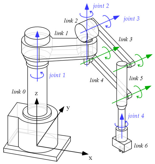
Figure 1.
The RRFbR SCARA-like architecture with elastic balancing (blue: actuated revolute joints; green: passive revolute joints).
The RRFbR architecture comprises seven links, from the base (link 0) to the end-effector (link 6). In Figure 1 the actuated joints (joint 1 to joint 4) are represented in blue. Joint 3 is the only actuated revolute joint of the four-bar mechanism; the remaining three passive revolute joints of the four-bar mechanism are represented in green. The axes of the actuated revolute joints 1, 2 and 4 are vertical; consequently, the corresponding motors are not loaded by gravity. On the contrary, the actuator of joint 3 is loaded by the gravitational forces acting on links 3 to 6. Therefore, to add a partial static balancing, reducing the torque of actuator 3 in steady state, a torsional spring can be added on joint 3, acting in parallel with actuator 3.
An alternative method to obtain static balancing involves adding a counterweight placed on link 3. Mass balancing and elastic balancing of the RRFbR architecture are compared in [21]. Mass balancing has the advantage of being exact for all angular positions of link 3, while elastic balancing is exact only for one angular position of actuator 3, and only approximated in the others. Nevertheless, elastic balancing reduces the inertial forces and avoids the encumbrance of the counterweight, with possible interferences with link 1 and with the environment; therefore, in the following only elastic balancing is considered.
Figure 2 shows the simplified kinematic scheme of the RRFbR architecture with elastic balancing. The internal coordinates are collected in the vector θ:
where θi is the angular position of the i-th actuated joint. The vector of the external coordinates collects the three components of the end-effector reference point E with respect to the origin of the fixed reference frame O(x,y,z) and the angle of rotation θ of the end-effector around the z axis (Figure 2):
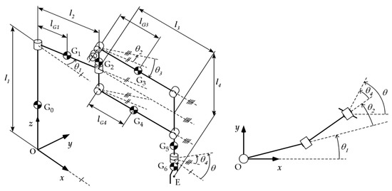
Figure 2.
Kinematic scheme of the RRFbR architecture with elastic balancing.
The direct position kinematics is expressed by the following expressions, which can be obtained from the geometry represented in Figure 2:
Deriving Equations (3)–(6) with respect to time, it is possible to obtain the Jacobian matrix, Equation (7), which expresses the direct velocity kinematics; in Equation (7), for brevity, si indicates sinθi, ci indicates cosθi and sij indicates sin(θi + θj):
In [21], the detailed dynamic model of the RRFbR architecture without static balancing is obtained by means of the Lagrange equations, neglecting friction in the joints:
where τi is the torque of the i-th actuator; L is the Lagrangian function, which is the difference of the kinetic energy Ec and of the gravitational energy Eg; Jji is the element (j,i) of the Jacobian matrix J and Fj is the j-th element of the vector F of the generalized forces applied by the end-effector on the environment, in the directions of the four external coordinates:
The expressions of the actuator torques (8), available in [21], are not reported here for the sake of brevity. The x and y components of the moment applied to the end-effector are supported by the joints and, in absence of friction, do not influence the actuation torques.
Introducing elastic balancing on joint 3, the third equation of system (8) becomes:
where k3 is the torsional spring stiffness and θ3p is the angular position of joint 3 at which the elastic return force of the spring is null. A good equilibration can be obtained imposing that in static conditions, with links 3 and 4 horizontal (θ3 = 0) and without payload, the spring moment exactly balances the gravitational effects acting on the robot arm, obtaining τ3 = 0; this can be obtained with a negative value of θ3p. This condition will be applied in the following.
Let us note that, depending on constructive requirements, the balancing spring can be placed on the actuated joint 3 or on another passive revolute joint of the four-bar mechanism without influencing the dynamic model; it is also possible to use more springs in parallel, distributing the stiffness on the four-bar joints. However, placing elastic elements only on the revolute joints connected to link 2, closer to the base, is favorable because it reduces the arm inertia.
3. KDHD Control of the RRFbR Robot
The classical KD impedance control/Cartesian space control with gravity compensation of the RRFbR arm is expressed by the following control law:
In Equation (11), the vector τ collects the four actuation torques (τ1 … τ4); xd is the time-varying vector of the set-point trajectory expressed in the external coordinates; the superscript (i) indicates the i-th-order time derivative; τg(θ) is the vector of the gravity compensation torques and KKD and DKD are the stiffness and damping matrices, which express the desired linear end-effector compliance.
In general, the matrices KKD and DKD, on the basis of the robot mobility, define the translational impedance, the rotational impedance or both [23]. In case of robots with Schoenflies motion, such as the RRFbR arm, their size is 4 × 4, and it is reasonable that the 1-DOF rotational behavior is decoupled from the translational behavior. Consequently, KKD and DKD are block-diagonal, with a 3 × 3 submatrix representing the translational impedance and the fourth diagonal element representing the rotational impedance.
Since gravity acts only on joint 3, as discussed in Section 2, all the elements of τg(θ) are null except the third, which has the following expression:
where mi is the mass of link i, lG3 and lG4 define the positions of the centers of mass of links 3 and 4, G3 and G4, and l3 is the length of the links 3 and 4 (Figure 2). In Equation (12) there is the sum of two terms; the second term takes into account the elastic return force of the balancing spring: the first term (negative, since the torque required to compensate gravity is opposite to the positive direction of θ3) is partially compensated by the action of the balancing spring, as desired, so the necessary gravity compensation torque τg,3 is reduced by the second term, usually positive, since θ3p < 0, as discussed in Section 2. Imposing exact static balancing (τg,3 = 0) when links 3 and 4 are horizontal (θ3 = 0) in Equation (12) leads to the following relationship, which can be used to define the spring parameters k3 and θ3p:
The KDHD control law is derived from the KD control law (11), with the addition of a damping term proportional through the half-derivative damping matrix HDKDHD to the half-derivative (derivative of order 1/2) of the external coordinates error:
Accordingly, the KD and KDHD control laws, (11) and (14), respectively extend the PD and PDD1/2 schemes from one dimension to the four-dimensional space of the Schoenflies motion. As discussed in [18,19], the half-derivative of a function of time f(t) can be calculated by using the following n-th order digital filter, derived from the Grünwald–Letnikov definition [24]:
where [y] indicates the integer part of y, and the n + 1 filter coefficients wj are:
The digital filter (15), which is used in the control law (14) to numerically evaluate the half-derivative of the error of the external coordinates, takes into account only the recent past of the derived function, in the interval [t–L, t]. In contrast, the exact calculation of an FO derivative involves the complete time history of the derived function. Consequently, Equation (15) introduces an approximation, which is usually accepted according to the short-memory principle [24]. Nevertheless, this approximation leads to an alteration of the end-effector stiffness, which should depend only on the stiffness matrix and not on the half-derivative matrix. To solve this problem, the following modification of the stiffness term can be introduced [18]:
The effectiveness of the stiffness compensation of the KDHD control law (17) was verified in [18,19]. The KDHD control law (17) will be compared in the following with the classical KD algorithm, expressed by Equation (11).
4. Dynamic Model of the RRFbR Arm with KD and KDHD Control
The KD and KDHD control laws were compared by means of the simulation environment Simscape MultibodyTM by MathWorks. The multibody model is shown in Figure 3, comprising two equal RRFbR manipulators, one with KD control and one with KDHD control, for a quicker comparison. The robots are subject only to gravitational forces. Friction in joints is neglected, in agreement with the analytical model discussed in Section 2.
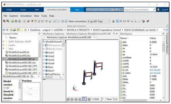
Figure 3.
Multibody model of the RRFbR manipulator.
Table 1 collects the main geometrical and mass parameters of the RRFbR arm that were used in the simulations.

Table 1.
Main geometrical parameters (Figure 2) and mass properties of the 3-PUU parallel robot.
In this comparison, a trajectory composed of six phases is considered. In each phase, the end-effector set-point position moves from the reference position xref along a direction parallel to one axis of the fixed reference frame O(x,y,z) for a distance d in a time tmov, stops at xref + Δx for a time tstop, then returns to xref in tmov and stops again for tstop, always keeping constant the end-effector orientation (θ = 0). The reference position xref is defined by the following internal coordinates: [−45°, 90°, 0°, −45°]; consequently, it corresponds to the robot arm semi-bent, in a central zone of the workspace. Moreover, in this position, links 3 and 4 are horizontal, and the gravity force action is compensated exactly by the balancing spring. The displacements Δx of the six phases are respectively (d, 0, 0), (0, d, 0), (0, 0, d), (−d, 0, 0), (0, −d, 0), (0, 0, −d). For each phase there is a gone and a return motion, with the same duration tmov, while the stops have duration tstop; therefore, the overall duration of the six phases is 12(tmov + tstop). Moreover, each motion is divided into three parts: acceleration, with duration αtmov; constant velocity, with duration (1–2α)tmov; and deceleration, with duration αtmov (s-curve motion). Consequently, the set-point motion is completely defined by the parameters d, tmov, tstop and α.
Figure 4 shows the set-point motion characterized by d = 0.15 m, tmov = 0.3 s, tstop = 1 s and α = 0.2, in terms of position, velocity and acceleration. These parameters correspond to trapezoidal velocity profiles of the displacements with maximum velocity of ±0.625 m/s. Acceleration alternates null values and constant values of ±10.416 m/s2 with duration αtmov = 0.06 s. This set point motion corresponds to the time histories of the internal coordinates shown in Figure 5.
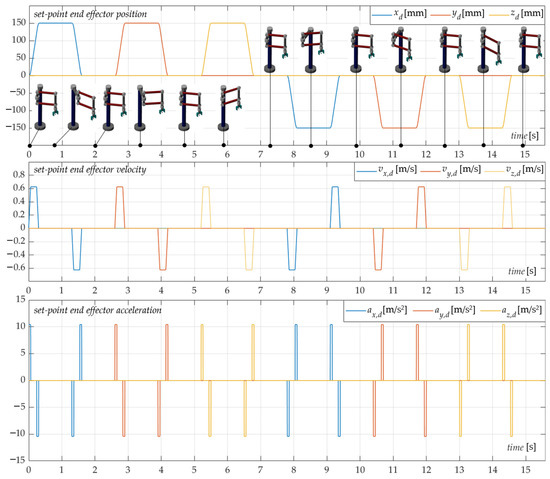
Figure 4.
Position, velocity and acceleration of the end-effector during the set-point motion.
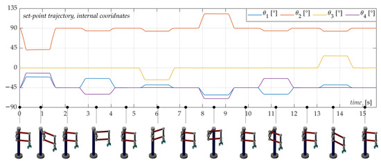
Figure 5.
Time histories of the internal coordinates during the set-point motion.
The end-effector orientation is kept constant along the planned motion. Nevertheless, this assumption does not limit the generality of the analysis because, as discussed in Section 3, it is reasonable to have the 1-DOF rotational behavior decoupled from the 3-DOF translational behavior, adopting block-diagonal stiffness and damping matrices. With this hypothesis and in absence of friction in the joints, the rotational behavior related to θ4 and τ4 is completely decoupled, and the tuning of the corresponding stiffness and damping matrix elements can be performed by the criteria already extensively discussed for the PDD1/2 control of SISO second-order linear systems [9,12].
5. Simulation Results
Figure 6 shows some synthetic results of the KD/KDHD comparison for the set-point motion of Figure 4 and Figure 5 (d = 0.15 m, tmov = 0.3 s, tstop = 1 s and α = 0.2). The considered sampling time is Ts = 5 ms and the filter order for the calculation of the half-derivatives is n = 10; these values are suitable for a real discrete-time implementation on a commercial controller. In this comparison, the Integral Control Effort (ICE) and the Integral Square Error (ISE) of the end-effector translational coordinates are compared:
where Tsim is a simulation time sufficiently long to take into account the residual vibrations. Moreover, in the comparison:
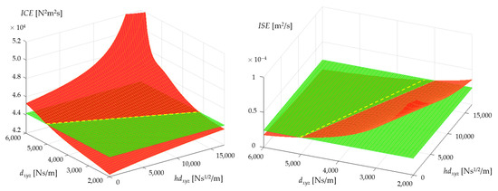
Figure 6.
Integral Control Effort (ICE) and Integral Square Error (ISE) as functions of the first-order translational damping dxyz and of the half-order translational damping hdxyz; the red surface is the KDHD control; the KD control is represented by the curves at hdxyz = 0 Ns1/2/m; the green horizontal planes indicate the ICE and ISE values of the KD control with dxyz = 5 · 103 Ns/m.
- For the KD control law, the stiffness matrix KKD is diagonal, with the first three diagonal elements kKD,x = kKD,y = kKD,z = 8·105 N/m, and kKD,θ = 5·102 Nm/rad; the damping matrix DKD is diagonal, with diagonal elements dKD,x = dKD,y = dKD,z = dxyz, and dKD,θ = 7.5 Nms/rad; and the translational damping dxyz is varied in the simulations in the range from 2·103 to 6·103 Ns/m;
- For the KDHD control law, the stiffness matrix KKDHD is again diagonal, and the elements kKDHD,x, kKDHD,y, kKDHD,z and kKDHD,θ are the same as in the KKD matrix, but with the addition of the stiffness compensation of Equation (17); the matrix DKDHD is diagonal, with diagonal elements dKD,x = dKD,y = dKD,z = dxyz, and dKD,θ = 3.75 Nms/rad; the matrix HDKDHD is also diagonal, with diagonal elements hdKDHD,x = hdKDHD,y = hdKDHD,z = hdxyz, and hdKDHD,θ = 2.4·104 Nms1/2/rad; in the simulations, the first-order translational damping dxyz varies from 2·103 to 6·103 Ns/m, and the half-order translational damping hdxyz varies from 0 to 1.7·104 Ns1/2/m.
Figure 6 shows in red the 3D graphs of the Integral Control Effort (left) and of the Integral Square Error (right) as functions of the first-order translational damping dxyz and of the half-order translational damping hdxyz; the intersections of these surfaces with the planes at hdxyz = 0 Ns1/2/m represent the KD behavior, without half-derivative damping.
From the analysis of Figure 6, it is possible to observe that increasing dxyz and hdxyz (that is, increasing the damping) leads to higher control effort and lower integral error. In order to evaluate the potential benefits of the KDHD control over the classical KD, the proposed method aims to assess if it is possible to obtain lower error using the same control effort. In Figure 6 (left), the green horizontal plane at 44,200 N2m2s represents the ICE value of the KD controller with dxyz = 5 · 103 Ns/m. This plane intersects the red surface of the KDHD Integral Control Effort with good approximation along a straight, yellow dotted line in Figure 6 (left). This straight line corresponds to this linear relationship between the translational first-order and half-order coefficients:
This means that the KDHD controllers fulfilling this relationship have approximately the same ICE as the original KD controller with dxyz = 5 · 103 Ns/m. Let us note that, according to relation (20), a decrease of the first-order damping is compensated by an increase of the half-order damping.
The trace of the linear relationship (20) is also represented in Figure 6 (right), on the horizontal plane which corresponds to 2.41 · 10−5 m2s, which is the ISE value of the KD controller with dxyz = 5·103 Ns/m. The red surface of the ISE of the KDHD control is lower than the green plane along the linear hdxyz–dxyz path for any positive value of hdxyz. This means that replacing an amount of first-order damping with some half-order damping reduces the Integral Square Error while keeping constant the Integral Control Effort.
This is confirmed by the plots in Figure 7, which show the ISE of the KDHD control (blue plot) and hdxyz (orange plot) as a function of dxyz, applying the linear relationship (20): as dxyz decreases from 5000 to 0 Ns/m and hdxyz increases from 0 (KD control) to 47,200 Ns1/2/m (KDHD control without first-order damping, named KHD), the Integral Square Error decreases from 2.41 · 10−5 m2s to 2.02 · 10−5 m2s (−16%).
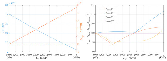
Figure 7.
Integral Square Error and half-order translational damping hdxyz as functions of the first-order translational damping dxyz (left); percentage maximum values of the actuation torques as functions of dxyz (right).
On the other hand, the complete replacement of the first-order damping with the half-order damping increases the maximum absolute values of the actuation torques, which are represented in Figure 7 (right) as percentages with respect to the KD control with dxyz = 5 · 103 Ns/m (τ4 is constant, due to the planned motion, with constant orientation of the end-effector).
A possible compromise to reduce the Integral Square Error while keeping nearly constant the maximum absolute values of the actuation torques is located near the middle (dxyz = 2.5 · 103 Ns/m, hdxyz = 23,600 Ns1/2/m).
Figure 8, Figure 9 and Figure 10 show the time histories of the errors of the translational external coordinates, ex, ey and ez, comparing:
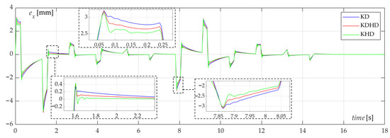
Figure 8.
Comparison of the KD (blue), KDHD (red), KHD (green) controls, error ex.
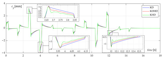
Figure 9.
Comparison of the KD (blue), KDHD (red), KHD (green) controls, error ey.
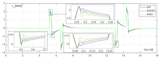
Figure 10.
Comparison of the KD (blue), KDHD (red), KHD (green) controllers, error ez.
- The KD control with dxyz = 5 · 103 Ns/m;
- The KDHD control with intermediate tuning (dxyz = 2.5 · 103 Ns/m, hdxyz = 23,600 Ns1/2/m);
- The KHD control with dxyz = 0 Ns/m and hdxyz = 47,200 Ns1/2/m.
Table 2 collects the main performance indexes for the three controllers. From the analysis of Figure 8, Figure 9 and Figure 10, and from the data collected in Table 2, it is possible to observe that the peak errors are similar for the three controllers, with a maximum reduction of −2.45% for the KHD with respect to KD (ey coordinate), but the mean errors decrease more remarkably moving from KD to KHD, coherently with the ISE plot in Figure 7 (left). In particular, the reductions of the mean absolute values of the translational errors with respect to KD are around −5 ÷ −6% for the KDHD, and −10 ÷ −11% for the KHD, while the Integral Square Error decreases were −8.7% for the KDHD and −16.2% for the KHD.
Table 2.
Comparison of the main performance indexes of the three controllers (KD, KDHD, KHD), with percentage variations of KDHD and KHD with respect to KD.
6. Discussion
The procedure used here to tune the KDHD control starting from a given KD control is applicable for a generic manipulator, and can be summarized as follows:
- A set-point motion, which covers a significant part of the workspace, is selected;
- Multibody simulations are performed varying the first-order translational damping dxyz and the half-order translational damping hdxyz, creating the 3D map of the ICE;
- The locus of the dxyz - hdxyz combinations with the same ICE of the given KD controller is identified;
- Simulations are performed along this dxyz–hdxyz path, starting from null hdxyz (KD control) and arriving at null dxyz (KHD control);
- Along this path, the main performance indexes (Integral Square Error, maximum and mean absolute values of the external coordinates error, maximum absolute values of the actuation torque) are evaluated, to select the KDHD tuning on the basis of a proper compromise;
- In general, a combination of first-order damping and half-derivative damping, intermediate between pure KD and pure KHD, makes it possible to reduce the tracking error with similar values of the maximum actuation torques, while the KHD has even lower tracking error, but also higher peaks of the actuation torques.
These outcomes are coherent with the results obtained for SISO systems controlled by means of the PDD1/2 scheme, for which a proper combination of first-order and half-order damping is preferable [9,25]. Nevertheless, the error reduction which can be achieved by introducing the half-order damping in Cartesian space control for the considered elastically balanced manipulator is much lower than the reduction achievable for a single mechatronic axis with inertial load, with equal maximum actuation torque of around −50% [26]. This is because in some phases the actuation torques must overcome not only the inertial forces, but also the elastic and gravitational forces, which are perfectly compensated only when links 3 and 4 are horizontal (θ3 = 0); these torque components are equal for the two controllers, and the half-derivative damping brings benefits only related to the transient behavior in the acceleration/deceleration phases; as a consequence, the overall performance benefit is lower with respect to an almost linear system with purely inertial load.
Some limitations of the proposed approach are as follows:
- The tuning is based on an arbitrarily selected set-point motion, which must be chosen in order to be representative of the typical working conditions;
- The first-order and half-order damping coefficients dxyz and hdxyz are imposed to be equal for the three translational external coordinates;
- The tuning of the rotational behavior is fixed.
In future research, these topics will be addressed in order to obtain more general results. However, the discussed simulation results confirm the potential benefits of fractional-order calculus, and in particular of the KDHD scheme, in the Cartesian space control of robotic manipulators. Moreover, an interesting research direction is the application to mechanisms with flexible links [27,28].
Author Contributions
L.B. conceived the control algorithm and designed the simulation campaign; S.E.N. developed the multibody model and performed simulations; L.B. and S.E.N. prepared the manuscript. All authors have read and agreed to the published version of the manuscript.
Funding
This research received no external funding.
Data Availability Statement
Data are contained within the article. The simulation data presented in this study are available in the figures and tables.
Conflicts of Interest
The authors declare no conflict of interest.
References
- Miller, K.S.; Ross, B. An Introduction to the Fractional Calculus and Fractional Differential Equations; John Wiley & Sons: New York, NY, USA, 1993. [Google Scholar]
- Hilfer, R. Applications of Fractional Calculus in Physics; World Scientific: Singapore, 2000. [Google Scholar]
- Rihan, F.A. Numerical modeling of Fractional-Order biological systems. Abstr. Appl. Anal. 2013, 2013, 816803. [Google Scholar] [CrossRef]
- Shaikh, A.S.; Shaikh, I.N.; Nisar, K.S. A mathematical model of COVID-19 using fractional derivative: Outbreak in India with dynamics of transmission and control. Adv. Differ. Equ. 2020, 2020, 373. [Google Scholar] [CrossRef] [PubMed]
- Sasso, M.; Palmieri, G.; Amodio, D. Application of fractional derivative models in linear viscoelastic problems. Mech. Time-Depend. Mater. 2011, 15, 367–387. [Google Scholar] [CrossRef]
- Podlubny, I. Fractional-Order systems and PIλDμ controllers. IEEE Trans. Autom. Control 1999, 44, 208–213. [Google Scholar] [CrossRef]
- Yeroglu, C.; Tan, N. Note on fractional-order proportional-integral-differential controller design. IET Control Theory Appl. 2012, 5, 1978–1989. [Google Scholar] [CrossRef]
- Beschi, M.; Padula, F.; Visioli, A. The generalised isodamping approach for robust fractional PID controllers design. Int. J. Control 2015, 90, 1157–1164. [Google Scholar] [CrossRef]
- Bruzzone, L.; Fanghella, P. Comparison of PDD1/2 and PDμ position controls of a second order linear system. In Proceedings of the IASTED International Conference on Modelling, Identification and Control, MIC 2014, Innsbruck, Austria, 17–19 February 2014; pp. 182–188. [Google Scholar] [CrossRef]
- Bruzzone, L.; Baggetta, M.; Fanghella, P. Fractional-Order PII1/2DD1/2 control: Theoretical aspects and application to a mechatronic axis. Appl. Sci. 2021, 11, 3631. [Google Scholar] [CrossRef]
- Jakovljevic, B.B.; Sekara, T.B.; Rapaic, M.R.; Jelicic, Z.D. On the distributed order PID controller. Int. J. Electron. Commun. 2017, 79, 94–101. [Google Scholar] [CrossRef]
- Bruzzone, L.; Fanghella, P. Fractional-order control of a micrometric linear axis. J. Control Sci. Eng. 2013, 2013, 947428. [Google Scholar] [CrossRef]
- Caccavale, F.; Siciliano, B.; Villani, L. Robot impedance control with Nondiagonal Stiffness. IEEE Trans. Autom. Control 1999, 44, 1943–1946. [Google Scholar] [CrossRef]
- Seraji, K. Cartesian control of robotic manipulators. In Proceedings of the IFAC 10th Triennial World Congress, Munich, Germany, 27–31 July 1987; pp. 289–294. [Google Scholar]
- Albu-Schäffer, A.; Hirzinger, G. Cartesian impedance control techniques for torque controlled light-weight robots. In Proceedings of the 2002 IEEE International Conference on Robotics & Automation, Washington, DC, USA, 11–15 May 2002; pp. 657–663. [Google Scholar]
- Kizir, S.; Elşavi, A. Position-based Fractional-Order impedance control of a 2 DOF serial manipulator. Robotica 2021, 39, 1560–1574. [Google Scholar] [CrossRef]
- Liu, X.; Wang, S.; Luo, Y. Fractional-Order impedance control design for robot manipulator. In Proceedings of the ASME 2021 International Design Engineering Technical Conferences and Computers and Information in Engineering Conference, Online, 17–19 August 2021; Volume 7, p. V007T07A028. [Google Scholar]
- Bruzzone, L.; Fanghella, P.; Basso, D. Application of the half-order derivative to impedance control of the 3-PUU parallel robot. Actuators 2022, 11, 45. [Google Scholar] [CrossRef]
- Bruzzone, L.; Polloni, A. Fractional Order KDHD impedance control of the Stewart Platform. Machines 2022, 10, 604. [Google Scholar] [CrossRef]
- Makino, H.; Furuya, N. Selective compliance assembly robot arm. In Proceedings of the First International Conference on Assembly Automation, Brighton, UK, 25–27 March 1980; pp. 77–86. [Google Scholar]
- Bruzzone, L.; Bozzini, G. A statically balanced SCARA-like industrial manipulator with high energetic efficiency. Meccanica 2011, 46, 771–784. [Google Scholar] [CrossRef]
- Hervé, J.M. The Lie group of rigid body displacements, a fundamental tool for mechanism design. Mech. Mach. Theory 1999, 34, 719–730. [Google Scholar] [CrossRef]
- Bruzzone, L.; Molfino, R.M. A geometric definition of rotational stiffness and damping applied to impedance control of parallel robots. Int. J. Robot. Autom. 2006, 21, 197–205. [Google Scholar] [CrossRef]
- Das, S. Functional Fractional Calculus; Springer: Berlin/Heidelberg, Germany, 2011. [Google Scholar]
- Bruzzone, L.; Bozzini, G. PDD1/2 control of purely inertial systems: Nondimensional analysis of the ramp response. In Proceedings of the IASTED International Conference on Modelling, Identification and Control, Innsbruck, Austria, 14–16 February 2011; pp. 308–315. [Google Scholar] [CrossRef]
- Bruzzone, L.; Fanghella, P.; Baggetta, M. Experimental assessment of fractional-order PDD1/2 control of a brushless DC motor with inertial load. Actuators 2020, 9, 13. [Google Scholar] [CrossRef]
- Boscariol, P.; Scalera, L.; Gasparetto, A. Nonlinear control of multibody flexible mechanisms: A model-free approach. Appl. Sci. 2021, 11, 1082. [Google Scholar] [CrossRef]
- Gupta, S.; Singh, A.P.; Deb, D.; Ozana, S. Kalman filter and variants for estimation in 2DOF serial flexible link and joint using Fractional Order PID controller. Appl. Sci. 2021, 11, 6693. [Google Scholar] [CrossRef]


Publisher’s Note: MDPI stays neutral with regard to jurisdictional claims in published maps and institutional affiliations. |
© 2022 by the authors. Licensee MDPI, Basel, Switzerland. This article is an open access article distributed under the terms and conditions of the Creative Commons Attribution (CC BY) license (https://creativecommons.org/licenses/by/4.0/).