Abstract
High-quality maps are pertinent to performing tasks requiring precision interaction with the environment. Current challenges with creating a high-precision map come from the need for both high pose accuracy and scan accuracy, and the goal of reliable autonomous performance of the task. In this paper, we propose a multistage framework to create a high-precision map of an environment which satisfies the targeted resolution and local accuracy by an autonomous mobile robot. The proposed framework consists of three steps. Each step is intended to aid in resolving the challenges faced by conventional approaches. In order to ensure the pose estimation is performed with high accuracy, a globally accurate coarse map of the environment is created using a conventional technique such as simultaneous localization and mapping or structure from motion with bundle adjustment. The high scan accuracy is ensured by planning a path for the robot to revisit the environment while maintaining a desired distance to all occupied regions. Since the map is to be created with targeted metrics, an online path replanning and pose refinement technique is proposed to autonomously achieve the metrics without compromising the pose and scan accuracy. The proposed framework was first validated on the ability to address the current challenges associated with accuracy through parametric studies of the proposed steps. The autonomous capability of the proposed framework was been demonstrated successfully in its use for a practical mission.
1. Introduction
Mapping of unknown environments is a fundamental task of engineering, which sees various valuable applications. They include the three-dimensional (3D) data storage [1], the monitoring [2], and the inspection [3] of existing structures and terrains. Maps can even be developed online for robots to navigate and complete their missions, such as search and rescue (SAR), in unknown environments. Robotic mapping is becoming ever more important due to the extensive potential that can be derived from high-precision results. If the mobile robot can develop a 3D map, it would reduce both time and human workload [4]. When the map is of high enough quality, it can be further used for inspection by creating a building information model (BIM) [5,6] or a digital twin [7] of the environment. Tasks that typically require real time vision can take advantage of a high-quality map, such as manipulation [8,9]. Since the uses of mapping are endless and evolving, the improvement in mapping resolution and accuracy can enhance the quality of work making use of mapping. The basis of this work was presented in part at International Workshop on Safety, Security, and Rescue Robotics (SSRR), Seville, Spain, November 2022 [10].
In order to create a map, the target qualities are first defined to optimize the process. Typically, the accuracy, resolution, and size of the completed map are targeted to a reasonable range of values. To significantly improve the mapping efforts, the resultant map should aim to have high quality metrics at both global and local levels. A single approach cannot target exceptional accuracy, resolution, and size at the same time, due to the limitations of current sensor technology, which usually has a trade-off between these metrics. Different mapping pipelines, as seen in Figure 1, may be used, but the conventional approaches plan the path of the robot and map the environment at the same time. These approaches are not able to leverage the strengths of different sensors and can only target one metric within a reasonable range, typically global accuracy. The proposed framework divides the problem into three distinct steps, allowing the strengths of different sensors to be leveraged to target multiple metrics.
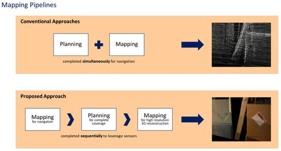
Figure 1.
The different mapping pipelines used to create a map of an unknown environment.
Past work on robotic mapping can be broadly classified into two approaches. The first is online robotic mapping techniques, such as simultaneous localization and mapping (SLAM) and its variants, where a robot entering an unknown environment iteratively builds up a map while also computing a continuous estimate of the robot’s location. The primary target is the global accuracy of the map, since the purpose of the created map is for successful robot navigation. This is a computationally costly process, since many SLAM algorithms will take advantage of both visual and internal sensors by fusing the data [11,12,13]. Therefore, SLAM algorithms typically focus on representing the environment in the most compact way in order to reduce the computational costs [14,15]. Maps are created primarily for successful robot navigation, where global accuracy is the major focus not the local resolution and accuracy. Improvements in map quality were made by fully representing the surface of interest in approaches typically classified as dense SLAM [16,17]. These methods produced high resolution and local accuracy, but the computational cost limits the scalable algorithms to small sized environments. These techniques work well for exploring unknown environments and creating a map to be used by a robot for future navigation.
While these approaches are well developed and are suitable for creating a map, there remains a gap between the focus of SLAM and creating a high-precision map. Since the objective of SLAM is to build a map of a completely unknown environment, the technique requires no prior knowledge, but the resultant map is typically sparse or locally inaccurate. In order to shift the quality of SLAM towards high-precision mapping, the environment must be explored thoroughly while considering the optimal viewing points. This exploration can be completed by using the next-best view approach for determining where optimal sensor observations are located. The unknown environment can be explored by analyzing frontier regions and predicted occlusions to determine the most optimal viewing location [18,19]. The results can be further improved by representing the scene as surfaces and revisiting the incomplete areas [20]. New techniques have been developed that make use of fixed manipulators and determining the best viewing positions inside the workspace in order to observe the entire environment [21,22,23]. The main issue with these techniques is that they rely on frontier identification and therefore do not know the whole environment during planning. This leads to areas being observed with different observation qualities, which is not sufficient to generate a consistent map of the scene. By coarsely exploring the environment and then navigating, the environment is able to be explored completely and uniformly with high accuracy.
The second class of mapping approaches is offline techniques, which use information from a set of images to build up a representation of the environment. Structure from Motion (SfM) can generate a 3D point cloud that corresponds to visually identified features from occupied regions of the environment by projecting the points from the image frame into Euclidean space [24]. In order to maximize the map accuracy, the SfM deploys bundle adjustment (BA), which globally minimizes the reprojection error [25,26]. The offline optimization allows larger environments to be accurately represented with 3D point clouds by making use of aerial images [27] and videos [28]. Neural radiance fields (NeRF) is an offline approach for generating high-resolution 3D viewpoints for an object, given a set of images and camera poses [29,30]. The key focus of NeRF is to efficiently represent the scene with implicit functions along viewing rays by outputting a density function relating to the lengths of the rays with colors associated with the position along a given ray. One of the practical issues with NeRF is the reliance on poses for each image which was originally computed using SfM [31], but new methods can learn the camera extrinsics [32,33] while creating the 3D model. Regardless of the methods for finding the camera extrinsics, the performance is hindered when high resolution is the goal, and the images must be captured near the surface of interest. If the room is able to be sampled with a hyper-resolution that is not conventionally achieved with SfM, the 3D reconstruction results can be greatly improved, as seen in Figure 2. Thus, the advantage of offline techniques is the global accuracy of the environment representation is unaffected by the environment size, as the 3D point cloud is computed offline through global optimization.
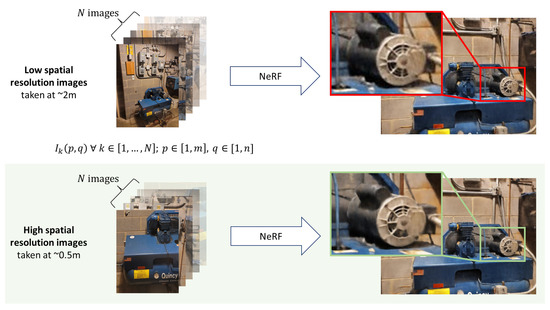
Figure 2.
The images and poses are used as inputs for NeRF [30] to generate a 3D rendering of the captured object. The standard set of images have a lower resolution in a unit area as compared to the images taken closer to surface. The differences in results are not too noticeable from the far viewpoint, but the differences can clearly be seen from the close viewpoint.
This paper presents a multistage framework to autonomously create a map of an environment using a mobile robot. Given an unknown environment, the task is to construct a high-quality map of the entire space autonomously. The quality of the map is given by the global accuracy and desired metrics—the aim being to maximize the quality. The proposed framework is divided into steps to specifically target the requirements needed to construct a high-quality map. The proposed framework consists of three steps that incrementally achieve the task by leveraging the strengths of different sensors and approaches. The first step (Step 1) constructs a coarse but globally accurate map by a conventional technique, such as SLAM (or SfM), by exploring an unknown environment with minimum motion. This provides a globally accurate skeleton of the environment to be used for path planning and pose estimation in the following steps. The second step (Step 2) plans a robot path which achieves the targeted distance. By having the resolution and local accuracy formulated in association with distance to the nearest structure, any point on the path is planned to have the targeted resolution and local accuracy. The targeted distance approximately guarantees the targeted metrics to control the quality of the resulting map. In the third step (Step 3), a path replanning technique directs the robot online to achieve the targeted resolution and local accuracy precisely. By replanning the path during the final step, the robot is able to autonomously record the data with the desired quality metrics. The strength of the proposed framework is its ability to autonomously create a high quality map without compromising the global and local quality of the map.
This paper is organized as follows. Section 2 describes the current mapping and exploration efforts, and the need for a multistage approach. Section 3 presents the multistage framework proposed in this paper for targeted sensor observations. Experimental validation, including parametric studies, is presented in Section 4, and Section 5 summarizes conclusions and ongoing work.
2. Mapping and Exploration
In order to create a high-precision map using an autonomous robot, both the mapping and exploration techniques must be state-of-the-art and reliable. The proposed framework will build on the fundamentals of mapping, to be discussed in the next subsection, in order to improve the map quality with predictability. For any mapping task, the resultant map of the environment must be complete, meaning all desired surfaces are properly observed. Therefore, complete coverage exploration, to be discussed in Section 2.2, is needed to thoroughly visit the entirety of the environment. Then, the limitations of the current approaches and how the proposed technique addresses those limitations will be discussed in Section 2.3.
2.1. Mapping of an Unknown Environment
A robot maps an unknown environment using a sensor suite that contains numerous sensors, including visual sensors, inertial sensors, encoders, etc. A typical configuration is a visual sensor that observes a local depth field and inertial sensors that measure changes in the robot pose. Given information on the initial pose of the robot and measurements from the sensors along the robot trajectory, the pose of the robot can be estimated. Since the goal of mapping is to output a two-dimensional (2D) or 3D map that represents the environment, the map is updated based on the pose estimation and measurement inputs from the sensors.
At a conceptual level, the problem of mapping an environment purely from information acquired by a set of sensors onboard a robot can be mathematically defined as follows. Let knowledge on the initial pose of the robot be . Information acquired by the depth sensor at time step k and the robot’s motion from to k measured by the inertial sensor are and , respectively. Given the estimate of the robot pose at by , the principle of the online mapping problem can be defined as updating the pose with the observations and :
where and are the sensor models associating the pose with the sensor output. and are the matrices that transform the sensor output into the pose, and substitutes the right-hand terms into the left-hand variable.
Once the pose has been identified and finalized over the time steps, the registration of the observations completes the mapping process. Registration is typically performed by either appending the incoming point cloud straight to the map or by a executing the iterative closest point (ICP) algorithm [34,35], as defined by:
where is the set of corresponding points; R is the rotation matrix; and t is the translation vector that transforms the incoming point cloud, , to the map point cloud, I. BA through global optimization is typically the last step to adjust and to increase the global accuracy by minimizing the reprojection error. The resulting point cloud which represents the map of the environment is given by .
2.2. Exploration and Navigation
The exploration of a known and unknown environment has numerous similarities, since the goal is the same, but the methods change to accommodate the differing amounts of prior knowledge. In order to create a complete map of the environment, the exploration must be performed using a variant of complete-coverage path planning [36]. Thus, the goal of exploration is to observe all of the desired surfaces in the environment with adequate certainty. Regardless of the method for exploration, the objective remains the same for exploring known and unknown environments.
When exploring an unknown environment, a map must be maintained to track the explored and unexplored regions of the environment. Typically, frontiers are then extracted from the map, and the robot will navigate through the environment until no more frontiers exist. This indicates the environment has been fully explored. When just considering the frontiers, the execution can be suboptimal, so the next-best view is used to improve the optimality of the path. By including information gain, the robot can observe the entire environment with minimal motion [37], which is desired to maintain high accuracy.
If the environment is known, then standard coverage path planning is easier, since the robot is just revisiting the environment. The planned path can be optimal, since the entirety of the scene is known. This also allows for path constraints to be followed more consistently than in frontier exploration. Common constraints for coverage path planning with respect to visual inspection include distance and orientation to the wall. Once all the viewing points which meet the specified criteria are selected, the points are connected by
where is the total path length to be minimized, is the distance between points and , and is 1 when the path connects and and 0 otherwise. The optimization problem can be formulated and solved using numerous techniques, including the genetic algorithm [38]. However, the dimensions of the basic formulation are too high to be reasonably solved without employing heuristics.
2.3. Need for a Multistage Approach
While the environment can be explored and a map can be created, the quality of the map is insufficient in two cases. The first case arises from the failure to cover all of surfaces with the depth-sensor measurements, . In the second case, there may exist a depth-sensor measurement, , which does not satisfy the targeted resolution. Both cases can occur when the 3D environment is considerably complex due to the changing geometry, even if a sophisticated Active SLAM technique is deployed. Since the low resolution is a result of measurement with distance, the local depth measurement may also be inaccurate. The map quality is insufficient in both the cases because the map becomes coarse. Even if a state-of-the-art exploration technique addresses these issues, standard SLAM techniques cannot be used to successfully create a fine map. This is due to the small number of geometric and visual features, which are used for pose estimation in many SLAM algorithms, being in the field of view of the sensor. Therefore, the pose estimation will likely be inaccurate even with the most robust SLAM techniques, and certainly unreliable. If the map is to be used to precisely represent the environment, the map must be accurate and have high spatial resolution to ensure all of the small details are recognizable.
The map created for global accuracy is generally poor in resolution and local accuracy, since both cannot be achieved simultaneously. This is due to the focus being on collecting scans with more information, such as geometric and visual features, which typically requires the sensor to be farther from to the surface. However, when creating a high-precision map, the sensor must observe the surfaces at a close distance to maintain high resolution and local accuracy. This indicates that a multimodal approach should be pursued when constructing a high-precision map to leverage the strengths of different sensors. All high-precision mapping approaches must be built on a coarse map with an emphasis on global accuracy. Only after a coarse map has been obtained can high-precision mapping be reliably achieved for large scales. The next section presents the multistage approach for autonomous robotic mapping proposed in this paper.
3. Autonomous Robotic Data Collection
Figure 3 shows the schematic diagram of the proposed multistage framework for creating a high-precision map. The proposed framework starts by creating a coarse global map developed by conventional mapping with minimum motion as a constraint and focuses on collecting data to create a map to achieve the targeted resolution and local accuracy with an autonomous robot. Minimum motion, such as a single loop around the environment, is used during coarse mapping to maintain the global accuracy by reducing the distance between pose estimations during SLAM or SfM. It is to be noted that the depth sensors of the proposed framework are a LiDAR, due to its high depth accuracy, and an RGB-D camera, due to its high aerial resolution. Consistent depth accuracy is needed in coarse global mapping because the robot may be away from the surrounding structures. This achieves global accuracy, though the robot must be close to its surrounding structures in the proposed framework to achieve the targeted resolution and local accuracy.
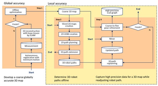
Figure 3.
The proposed multistage approach for autonomous high-precision mapping consists of three steps. Step 1 constructs a globally accurate coarse map to be used in the latter steps. Steps 1 and 2 use the coarse map to as prior information to focus on high precision. Step 2 plans a path for the robot observations to achieve the desired metrics. Step 3 adjusts the path to assure the metrics are met and the data are suitable for high precision mapping.
The proposed framework consists of three steps. The first step, Step 1, autonomously constructs a globally accurate coarse map of the environment to be used in the succeeding steps. In order to create a globally accurate coarse map, a 3D LiDAR is used for its consistent depth uncertainty and large range. The coarse map is created by using a conventional mapping technique, such as SLAM, and having the robot navigate through the unexplored environment with minimum motion. Since the proposed technique will later have the robot revisit the entire environment for high-precision observations, the coarse map does not have to be locally complete but should be globally complete.
The second step, Step 2, plans a 3D path of the robot offline, which maintains the desired distance to the nearest structure of the environment and approximately guarantees the minimum desired resolution and accuracy. Objects in an indoor environment can be generically classified as horizontal or vertical surfaces. Major horizontal surfaces include the floor and ceiling. Vertical surfaces mostly consist of the walls and other objects extending upwards from the floor. Therefore, planning is done separately for the horizontal and vertical surfaces. Since the indoor environment is most often designed with horizontally stretched space, the coarse global map is first sliced into multiple horizontal 2D planes, each with a different height, and an occupancy grid map (OGM) is created for each 2D plane. Planes representing the floor and ceiling are then used for planning revisiting major horizontal surfaces. This planning consists of basic-area-coverage path planning, so that the robot can revisit the entirety of the floor and ceiling for complete coverage. The remaining planes are used for planning the path for the robot to revisit the vertical surfaces. The proposed framework creates a unoccupancy distance map (UDM) for each OGM and identifies pixels of the UDM image that have the desired distance to the nearest structure. The pixels of each layer are connected using a reduced-order travelling salesman problem (TSP) technique and results in the 2D path of the robot of the layer. In the final process of Step 2, the 2D paths are connected so that the robot covers the 3D space in a single trip.
Step 3 replans a path and constructs a scan graph with RGB-D camera measurements online. While the offline path is concerned only with the distance to the nearest structure, the path replanned online navigates the robot such that the final data satisfies the targeted resolution and local accuracy. The robot moves not only to collect the expected data but also explores areas that were not identified in coarse global mapping. This online path optimization is necessary to correct the predictions made in Step 2 approximating the resolution and local accuracy. Step 3 not only ensures the targeted resolution and local accuracy, but also the coverage completeness. Once the robot has moved, the RGB-D camera measurements are aligned to finalize the pose estimations from coarse to fine. The process continues until the robot completes all of the data collection.
3.1. Step 1: Globally Accurate Coarse Mapping
The first requirement, for creating a high-precision map, is to create a globally accurate coarse map of the environment. If the map of the environment is known, from previous exploration or a BIM [39], and the results are globally accurate, then Step 1 can be skipped. In the cases where the environment is unknown, Step 1 is used to create a map of the environment with a focus on global accuracy.
To construct a map with high global accuracy, a rotating 3D LiDAR is used for its wide field of view, large range, and consistent error with respect to distance. Basic frontier exploration [40,41] is used to navigate through the environment to create a globally complete map. The exploration does not have to lead to a locally complete map, so the focus can be on reliable exploration with minimum motion. Since the objective of Step 1 is to maximize the global accuracy, there is a desire to minimize motion of the robot to reduce errors associated with pose estimation by considering the information gain associated with the next planned position. During exploration, a generic 3D SLAM algorithm [42,43], with support for a variety of sensors, is used to construct the globally accurate 3D map. Since many SLAM techniques rely on feature matching, the angular velocity of the sensor should be minimized to reduce the changes in position of tracked features. The resultant map will be globally complete and accurate—a suitable map for planning and navigation.
3.2. Step 2: Offline 3D Path Planning for Complete Surface Coverage
Step 2 of the proposed framework aims for the targeted resolution and local accuracy to be achieved by planning the path of the robot so that its corresponding targeted distance to the nearest structure of the environment is maintained. For offline path planning, the resolution and local accuracy at each point can only be predicted. The generic setup for the offline prediction for path planning can be seen in Figure 4, which details the sensor field of view projected onto a wall in the environment. The spatial resolution and accuracy of a visual sensor are inversely proportional to measuring distance. Small distances imply higher spatial resolution and accuracy. Spatial resolution of a theoretical scan near a planar surface can be given by
where is the sensor resolution, is the field of view, and d is the distance to the center of the measurement. The accuracy is not easily defined, so conversely, the error of the depth measurement can be used instead. The depth error is typically given as a proportion of the sensor reading, so the predicted error is
where is the reported accuracy. The targeted distance, , represents is the estimated distance to achieve the targeted resolution and local accuracy. It can be estimated by
where is the targeted spatial resolution, is the targeted error, and and are the scaling factors.
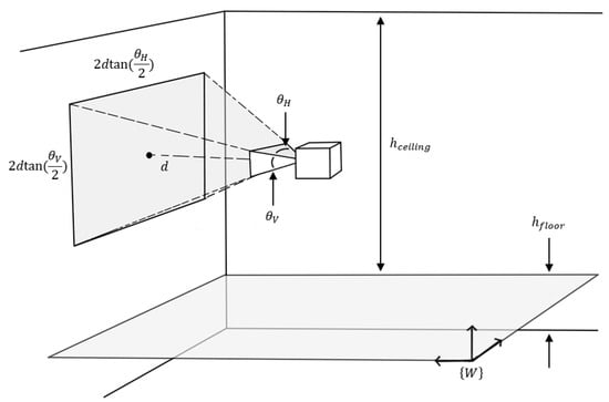
Figure 4.
Diagram of an indoor environment with a depth sensor making an observation on a planar wall.
To ensure that autonomous path planning does not fail in a complex 3D environment and being aware that the indoor space is stretched horizontally, the robot is planned to revisit the entire 3D space by moving horizontally at different heights. The observation height for the floor, , and ceiling, , are defined by
where is the height of the floor and is the height of the ceiling. Since the aim of the proposed technique includes coverage completeness, a unit viewing area will be defined for the sensor. This ensures that regardless of the orientation about the viewing axis, everything in the unit viewing area is observed. The unit viewing dimension is calculated by rotating the field of view about the center point and inscribing a circle, as seen in Figure 5. A square was then inscribed in the circle to determine the unit viewing area at the targeted distance, as given by
where is the unit length of the unit viewing square.
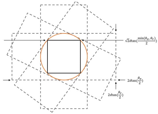
Figure 5.
Unit viewing area for a sensor at a given distance, given by rotating the field of view and inscribing a square into the union of all of the fields of view.
The number of horizontal slices, , corresponding the major vertical surfaces depends on the height of the environment and field of view of the sensor. It is given by
where is the ceiling operator. Since the number of layers must be an integer, the ceiling operator is used instead of the rounding operator or the floor operator to ensure that the entire vertical surface is observed. The different layer heights, , are
where the heights are evenly distributed from the floor to the ceiling.
Let the ith grid of the 2D OGM created by slicing the coarse global 3D map of the conventional mapping at the defined heights be
where is a occupancy grid mapping operator. The OGM conventionally outputs the values of 0, 1/2, and 1 for occupied, unexplored, and unoccupied grids, respectively. The proposed framework re-expresses the OGM as the Euclidean UDM towards planning a 3D path offline and returns an unoccupancy distance as:
where is a revised version of the OGM operator that outputs the distance of the grid from the nearest occupied grid. The distance in the UDM is 0 when the grid is “unexplored” in addition to “occupied”. The state of “unexplored” is treated equally to the “occupied” because the path cannot be planned in unexplored areas. Figure 6 illustrates the OGM and the UDM comparatively. It is seen that the primary aim of the UDM is to map distance in unoccupied space.
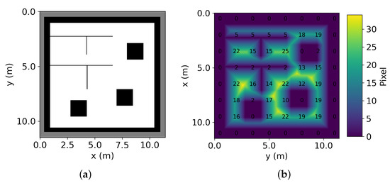
Figure 6.
Resultant OGM (a) and UDM (b) created from the coarse map.
For map slices representing the major horizontal surface, which corresponds to the floor or ceiling, the robot needs to revisit the entire available area. This is also known as coverage path planning. Typically, the environment is discretized in a grid map, and each grid cell is a point for the robot to visit. Since the aim of the proposed framework is to map the entire surface at a specified distance, , the grid cells can be resized to correspond to the field of view of the sensor. Simply, the grid cells will be resized to match the unit viewing length. By using the minimum dimension of the sensor field of view, it ensures that regardless of the orientation the entire area of the grid cell will be observed.
After the OGM has been resized, with the grid cells being roughly the same size as the sensor field of view, a simple coverage path planning algorithm can be used. A variety of techniques can be used to visit each cell, each with different optimality criteria. This approach uses the boustrophedon technique [44] to plan a path through each cell due to its many straight paths, which will minimize unnecessary change in motion for most of the environment. The path planning technique just connects all of the points together into a single path; the sensor orientation is not considered until after the path is complete. Since the motion and the surfaces of interest are in parallel planes, the sensor orientation is constant for the entire path with the sensor facing the surface of interest.
The remaining map slices will correspond with the major vertical surfaces, primarily the walls, so the robot needs to follow the perimeter of the map. The proposed framework then identifies the grids of the UDM or the pixels of its image that have the targeted distance to the nearest structure. Let be the pixel of the structure nearest to the pixel . The condition of the pixel to be a waypoint of the path is
where indicates the norm throughout the paper, and is the distance between the two neighboring pixels or the pixel resolution. A pixel is chosen within the pixel resolution to select the pixels that are necessary to pass through. Figure 7 shows the pixels selected to compose an offline path.
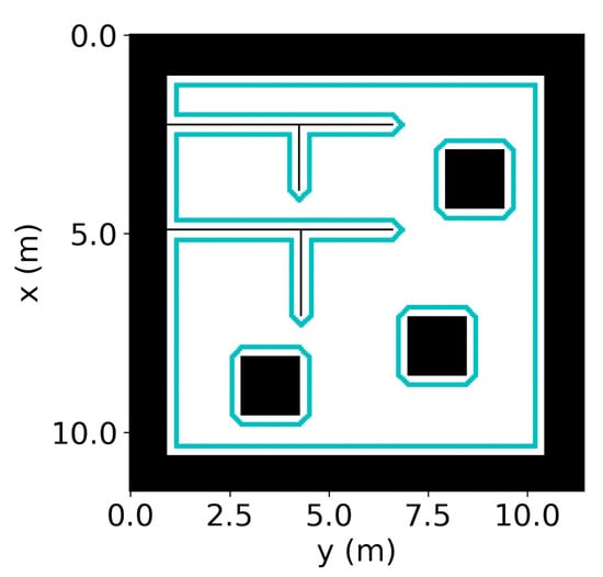
Figure 7.
Pixels (cyan color) selected to make up the offline path.
Since they are not connected, the pixels should form a path by connecting themselves but with minimum overlaps. While problems for finding a path to visit all the waypoints with minimum overlaps are known as TSP, the number of points is so large that this problem cannot be solved by plain TSP solvers in a reasonable time. The problem of concern has the following unique constraint: Pixels representing the boundary of each structure are located near each other and sequentially expand along the contour. Thus, pixels along the boundary can be connected as segments of the planned path.
The proposed framework first connects the points near each other as segments. In this way, the dimension of path planning is significantly reduced, since the problem is now defined as finding the order of start and end pixels of the segments to visit. Let the end pixel of the ith segment and the start pixel of the jth segment be and , respectively. In accordance with the TSP, the problem is formulated as
where and . is the distance from the end pixel of the ith segment to the start pixel of jth segment . , which takes one if and are connected as a part of the path. The Dantzig–Fulkerson–Johnson formulation [45] adds the following constraints to complete the problem, ensuring each and every point is visited once with no subtours:
where Q is a subset. Solving the problem is to decide the values of . The proposed framework calculates based on Euclidean distance for fast computation. Since the number of segments is not large, this TSP problem can be solved using either exact algorithms [46] or heuristic algorithms [47]. After has been decided, the path from to in which is planned to avoid obstacles by common motion planning algorithms, such as A star and D star [48]. The desired sensor orientation is added to each of the points along the path by obtaining the normal of n nearest occupied pixels. The normal of the pixels is computed by using random sample consensus (RANSAC) [49] to fit a line through the points and finding an orthogonal direction vector by
where m is the slope computed from RANSAC, is the normal angle, and v is the direction vector for the sensor.
Figure 8 shows the resulting 3D path created after the 3D expansion. Since a 2D path is developed for each horizontal plane, the 3D expansion is completed by connecting a path point of one horizontal plane to a path point of the next horizontal plane.
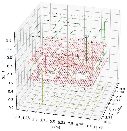
Figure 8.
Resulting 3D offline path of a room with two horizontal layers (red paths) and three vertical layers (green paths). The object located at does not reach the upper-most layer.
3.3. Step 3: Online Path Optimization for Targeted Metrics
The path planned in Step 2 only approximately guarantees the resolution and local accuracy because the offline path is concerned only with the distance to the nearest structure. Therefore, as the path is followed by the robot using localization from the rotating 3D LiDAR, the path is replanned and controlled online based on the measured resolution and local accuracy. The online path optimization guarantees the map is finalized with the targeted resolution and local accuracy. To evaluate the resolution at a macroscopic scale, the proposed framework defines it in terms of pixel density. Suppose that the structure’s surface of concern for the robot at time step k is . If the number of pixels from the data to exhibit the surface is , the pixel density of the surface, , is given by
.
The local accuracy, on the other hand, can be evaluated in terms of the characteristics of indoor structures. Since the surface of the indoor structure is geometric, poor local accuracy is often identified by the fluctuation of pixel locations. Let the mean deviation of the ith pixel and the neighboring pixels from the fit plane be . The mean deviation of the surface of concern is given by
The objective of the online path optimization in Step 3 is to find the incremental motion that follows the path planned in the Step 2 offline planning and improves the resolution and the local accuracy:
where is the next desired robot pose along the path, and is the currently estimated robot pose. The control objective is subject to constraints so that the map meets the minimum criteria at time step :
The resolution and the local accuracy that the robot achieves in the actual mission would differ from the predicted values in Step 2. This necessitates the path replanning to ensure the targeted resolution and local accuracy are maintained.
Various sophisticated solutions are available for constrained nonlinear optimization, but the problem of concern with a linear objective function and light convex constraints can be solved relatively straightforwardly. The proposed framework adopts a conventionally accepted solution [50] and solves the problem by reformulating the objective function with penalties as
where and are the scaling factors.
Since the pose is initially estimated by the rotating 3D LiDAR, the measurements have high uncertainty, which is not suitable for high-precision mapping. The pose refinement is performed through the alignment of the RGB-D camera point cloud to the coarse map. Since the coarse map is globally accurate and there is an initial estimate of the camera pose, the alignment of the RGB-D camera point cloud is also straightforward.
The newly observed point cloud should be matched to the preceding map point cloud through the ICP method to find the rigid transformation, , between the coarse map points, , and the new RGB-D points, . The pose composed by the Step 2 planned path and Step 3 replanning is measured by the rotating 3D LiDAR and converted to an matrix, , to be used as the initial conditions for registration. The registration is performed as follows to find the pose of the new point cloud:
The incoming RGB-D point cloud is successfully aligned to the preceding coarse map by applying the transformations. The resultant pose from the aligment is represent by:
where is the refined pose estimate from the ICP refinement. By matching the incoming RGB-D point clouds to the prior LiDAR point cloud, the computation is reduced while maintaining global accuracy, since the global structure is already present.
4. Numerical/Experimental Validation
The proposed framework of autonomous data collection was tested and validated through parametric studies and a real-world application. Section 4.1 investigates the path planning of Step 2 with synthetic maps which were generated by positioning different kinds of objects on given grid maps. Section 4.2 studies the quality of collected data parametrically after the Step 3 online map refinement. The autonomous mission of the proposed technique in a practical environment is demonstrated in Section 4.3.
4.1. Planning Performance of Step 2
The performance of the reduced-order TSP planning technique, for vertical observations, was assessed for completion and time during validation. The other parts of Step 2 were not tested, as the TSP is newly proposed. Table 1 lists the parameters used for path planning of Step 2. The synthetic maps were generated by positioning three kinds of objects (square, circle, and triangle) on a given map of random size. The object may or may not appear on each map, and the position and rotation of each object are also random.

Table 1.
Parameters of the Step 2 validation.
Figure 9 shows two examples of the synthetic map and the planned paths. The dynamically sequential movement along the path is shown by the arrows indicated along the path. In the test, paths were successfully planned for all of the generated environments. Since the motion planning algorithm is needed to link the endpoints of two disconnected segments, if many pairs of endpoints need to be connected, the planning would take a considerable amount of time.
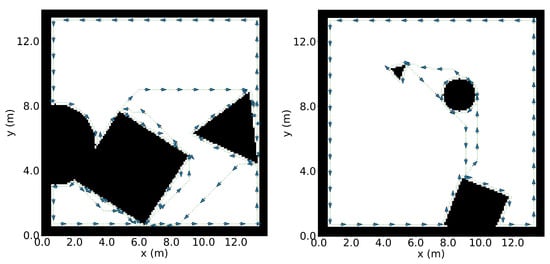
Figure 9.
Two examples of synthetic maps used for the validation of Step 2. The planned paths are indicated with the dotted lines around the objects, and the arrows show the sequential movement.
Figure 10 shows box plots of the computational time with respect to the map size and the number of objects positioned in the environment. The computational time is defined as the time taken for completion of the section of Step 2 for vertical observations, including: preprocessing of distance transform, solving TSP, and D star motion planning. The computational time of planning was recorded for all 200 maps. The mean computational time increased as the map size and the number of objects became larger. This is because the motion planning consumes more time when the map is bigger and the environment is more complex due to more positioned objects. The motion planning took the majority of the time— of the entire time.
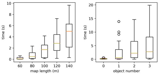
Figure 10.
Box plots of the computationaltime with respect to the map size and the object number in the environment.
4.2. Local Metric Evaluation of Structure from Step 3
In order to test the validity of Step 3, a known and controlled environment was constructed for repeatable testing and comparisons. As per Step 1, a globally accurate coarse map was constructed using a rotating LiDAR given its precise measurement, irrespective of the distance. A path was not planned using Step 2, as the purposed of this experiment was to test the performance of Step 3 to achieve the desired metrics. The robot was instructed to move past the objects at an approximate distance with the online optimization to be followed to guarantee the desired metrics. For Step 3, a depth camera was added, as its measurement precision was ensured when the objects were near, which was ensured by following the path of Step 2.
The main focus of the parametric study was to quantitatively determine the resolution and local accuracy of the proposed framework. Since the resolution is a function of the 3D reconstruction method, which can sometimes include interpolating functions, the resolution was compared to the desired resolution used in Step 3. The local accuracy was compared to conventional techniques to determine the effectiveness of the pose estimation. A standard SLAM package, RTAB-Map [42], was used as the conventional mapping technique using the default recommended parameters for each respective sensor. Table 2 describes the desired metrics, sensor distance, and other parameters used to during the experiment. An approximate distance, similar to the value calculated in Step 2, was used to determine whether the online optimization was necessary. The same path was followed at a distance of 1.25 m for all sensors. The distance was chosen so both the LiDAR and the depth camera could maintain global accuracy, as moving closer would disrupt the pose prediction and registration of conventional techniques. The local accuracy and resolution were tested on the same surfaces, as shown in Figure 11, located within a room, so all sensors could ensure adequate evaluation. A ground truth model was created by measuring the environment and drafting a CAD model for comparison.
Table 2.
Parameters of the validation of Step 3.
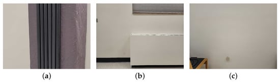
Figure 11.
Known structures for testing the resolution and local accuracy of the proposed method. (a) Periodic surface, (b) non-periodic surface, (c) flat surface.
The results of the study fully validate Step 3 by showing consistently high resolution and local accuracy on all of the test structures. Resolution was calculated by finding the distance between every point and its nearest neighbor, with the goal being to have as small a distance as possible. Figure 12 shows the higher resolution of the point cloud while using the proposed framework, with all points being within 1 mm of their nearest neighbors. The local accuracy was computed by comparing the resultant point cloud to the ground truth 3D model of the structures of interest. The point clouds of the collected data were assembled using basic registration of the point clouds from the computed poses. The point cloud was sliced horizontally to generate more samples so the accuracy could be individually compared among varying heights. As seen in Figure 13, the local accuracy of the proposed framework is significantly better than that of the ICP odometry and at least as good as that of the RGB odometry. These are optimal results as the local accuracy of the proposed framework is similar to the reported values on the sensor data sheet.
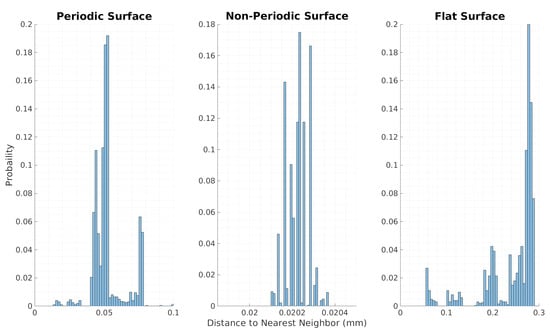
Figure 12.
Histogram of local resolution for the controlled environments.
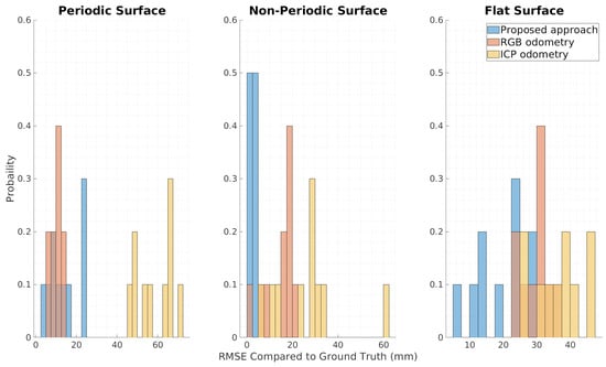
Figure 13.
Histogram of local accuracy for the controlled environments.
4.3. Autonomous Map Creation of a Practical Environment
Figure 14 shows the robot and the indoor environment that were used for the real-world experiment. The robot consisted of a wheeled platform and a manipulator on top of it. Both the 3D LiDAR and the depth camera were attached to the end of the manipulator. The manipulator allows the positioning of the sensors in 3D space, which allows for the creation of a high-precision map. The indoor environment is a typical workplace office that has various furniture facing the wall and an open area. Since the furniture does not go all of the way to the ceiling, the sliced 2D maps differ depending on the height.
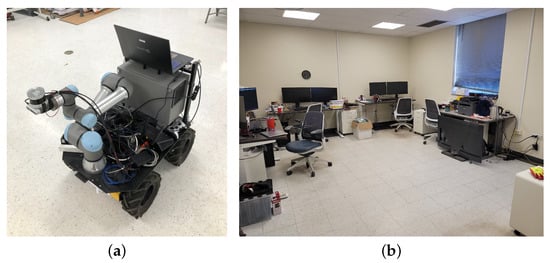
Figure 14.
UGV used for map refinement and the environment of the real-world experiment. (a) UGV with manipulator, (b) Test environment obstacles and furniture.
Table A1 lists the input parameters of the experiment. The SLAM package for coarse mapping and sensors was not changed from the experiment in Section 4.2. Figure A1 shows the point cloud of the coarse map used in the pose refinement. The map shows global accuracy as the boundary of the room is square, indicating it is well loop-closed. The occupancy grid maps of different heights were generated, as seen in Figure A2, and used as the inputs to the proposed framework. The OGMs are seen to differ from each other to some extent due to the presence of structures at different heights, confirming the need for path planning at each height. The UDMs in Figure A3, selected pixels for the traversal in Figure A4, the path planned for each layer in Figure A5, and the computed values in Table A2, are shown for completeness.
Figure 15 shows the final 3D offline path computed by Step 2. It is to be noted that some of the z values are negative, since the origin of the map is located 1.68 m above the ground, where the coarse mapping began. The heights of the floor and ceiling are indicated in Table A2, which control the range of the heights used for the planned path. The path was followed by the robot to traverse the environment and refine the coarse map. The ROS1 navigation stack with move_basewas used as the backbone for movement of the mobile platform. The robot arm extended to reach the different layers and moved to perform fine motion corrections. While the path planning for synthetic maps was always successful, following the path depends on more factors. The performance of the path following is restricted by the dynamic and kinematic constraints of the mobile robot. For instance, the robot became stuck sometimes in positions when the distances to objects were set to be too small due to the non-holonomic constraints provided by the mobile robot. If a robot has holonomic constraints, such as a mobile robot with mecanum wheels or a hexacopter, the ability to recover motion in tight spaces is improved.
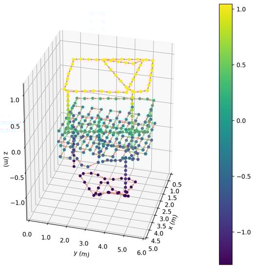
Figure 15.
Resulting 3D offline path created during Step 2.
Figure 16 shows a section of the map generated by NeRF [30] after using the proposed framework. Different pose estimation techniques were used to compute the poses necessary for NeRF. The proposed framework was tested alongside commonly used techniques, such as COLMAP [31] and LiDAR localization. The practical test was repeated in other environments with different layouts to determine the robustness of the proposed framework. The test environments were a machine room, as seen in Figure A6, a robotics laboratory, as seen in Figure A7, and a nuclear reactor’s silo, as seen in Figure A8. For these, the maps are represented by the point clouds registered together at the respective refined poses computed from Step 3. The machine room is small and unstructured environment, proving the proposed approach can handle tight enclosed spaces. The robotics laboratory is large and horizontally stretched, the horizontal mapping layers are well suited for environments of this type. The nuclear reactor’s silo is vertically high, showing the capabilities even when the structure is tall. It is to be noted that there is no ceiling for the high-precision map due to the height of the structure, and the LiDAR point cloud remains to show the skeleton structure of the space. The performances in many different environments show the proposed framework can be used in many real-world settings and applications.
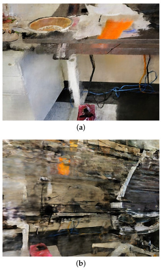
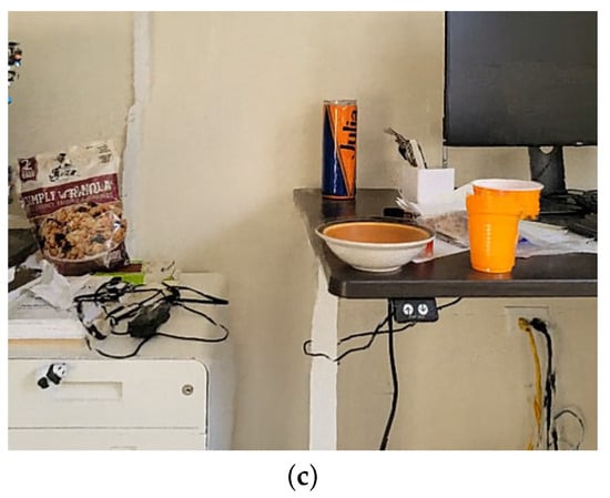
Figure 16.
Comparisons of the resulting NeRF [30] renderings using different techniques to estimate the poses of the images. (a) Poses generated with COLMAP [31]. (b) Poses generated with ICP localization using a rotating 3D LiDAR. (c) Poses generated using the proposed multistage framework.
As predicted, the pose estimation of the conventional techniques is not suitable for collecting images with high spatial resolution. As shown similarly in the parametric study, the low local accuracy and resolution of the conventional techniques can leave surfaces blurry and unidentifiable. However, the proposed framework is able to create a map that is clearly recognizable due to the verifiable high local accuracy and resolution.
5. Conclusions
This paper has presented a multistage framework for high-precision autonomous robotic map creation. Each step focuses on alleviating a specific common challenge; thus, the strengths of each step ensure the map quality meets the target specifications. The first step creates a map with conventional mapping techniques to focus on global pose estimation accuracy. Step 2 plans a desirable path for the robot to revisit the environment while maintaining a desired distance to all objects of interest. Since the distance approximates the predicted resolution and local accuracy that will be achieved by the sensor, following the path ensures the scan accuracy is high. The framework is made autonomous by replanning the path to achieve the targeted metrics while creating the high-precision map. The pose estimates are also refined in Step 3 to maintain high precision for all of the mapping data.
In this paper, it was found that the steps of the multistage framework are able to improve the results related to the challenges associated with the current mapping efforts. The pose and scan accuracy were validated for the proposed framework with parametric studies testing the planning and execution performance. The final practical experiment validated the autonomous capabilities of the proposed framework through testing in different types of environments. The performance of the framework was not hindered in any off the environments, thereby confirming the practical usefulness of the framework.
We focused on the high-precision mapping capability as the first step, and much work is left open for future research. Ongoing work includes the reduced-order map representation and its application to inspection and maintenance. Work is also being done on semantic segmentation of static and dynamic objects in the environment to aid robot interactions. New results will be presented through the upcoming opportunities, including conferences and journal papers.
Author Contributions
Conceptualization, W.S., Y.Q., S.S., T.F. and G.D.; data curation, W.S., Y.Q., S.S. and H.B.; formal analysis, W.S. and Y.Q.; funding acquisition, T.F.; investigation, W.S.; methodology, W.S., Y.Q., S.S., T.F. and G.D.; project administration, W.S. and T.F.; resources, T.F.; software, W.S., Y.Q. and H.B.; Supervision, T.F.; validation, W.S. and Y.Q.; visualization, W.S. and Y.Q.; writing—original draft, W.S., Y.Q. and T.F.; writing—review and editing, W.S., Y.Q., S.S. and T.F. All authors have read and agreed to the published version of the manuscript.
Funding
This work is sponsored by US Office of Naval Research (N00014-20-1-2468) and THK Co., Ltd.
Acknowledgments
The authors would like to express their sincere gratitude to Tom McKenna and Jun Kawasaki for their invaluable support and advice.
Conflicts of Interest
The authors declare no conflict of interest. The funders had no role in the design of the study; in the collection, analyses, or interpretation of data; in the writing of the manuscript; or in the decision to publish the results.
Appendix A. Step 2 Data for a Practical Office Environment
Appendix A.1. Globally Accurate Coarse Map

Figure A1.
Coarse global map created using the conventional SLAM technique (RTAB-Map [42]).
Figure A1.
Coarse global map created using the conventional SLAM technique (RTAB-Map [42]).

Appendix A.2. Parameters and Calculated Values
Table A1.
Input parameters of the real-world experiment.
Table A1.
Input parameters of the real-world experiment.
| Parameter | Value |
|---|---|
| (mm) | 1 |
| (pixel/mm) | 1 |
| Coarse map SLAM package | RTAB-Map [42] |
| 3D LiDAR | Ouster OS1-16 |
| Depth camera | Intel L515 |
| H (deg) | 70 |
| V (deg) | 43 |
| (%) | 0.155 |
| m by n (pixels) | 1080 × 1920 |
| , | 1, 1 |
Table A2.
Computed parameters of the real-world experiment.
Table A2.
Computed parameters of the real-world experiment.
| Parameter | Value |
|---|---|
| (m) | 1.46 |
| (m) | −1.68 |
| (m) | 1.44 |
| , (m) | −0.222, −0.0253 |
| (m) | 0.814 |
| (layers) | 4 |
| (m) | −1.29, −0.514, 0.266, 1.04 |
Appendix A.3. Occupancy Grid Maps (OGMs)

Figure A2.
OGMs of the test environment at different layers. (a) Floor layer ( m). (b) Ceiling layer ( m). (c) First layer ( m). (d) Second layer ( m). (e) Third layer ( m). (f) Fourth layer ( m).
Figure A2.
OGMs of the test environment at different layers. (a) Floor layer ( m). (b) Ceiling layer ( m). (c) First layer ( m). (d) Second layer ( m). (e) Third layer ( m). (f) Fourth layer ( m).

Appendix A.4. Unoccupancy Distance Maps (UDMs)

Figure A3.
UDMs of the test environment at different layers. (a) First layer ( m). (b) Second layer ( m). (c) Third layer ( m). (d) Fourth layer ( m).
Figure A3.
UDMs of the test environment at different layers. (a) First layer ( m). (b) Second layer ( m). (c) Third layer ( m). (d) Fourth layer ( m).

Appendix A.5. Pixels Selected for Path Planning

Figure A4.
Pixels selected to compose the path for the test environment at different layers. (a) First layer ( m). (b) Second layer ( m). (c) Third layer ( m). (d) Fourth layer ( m).
Figure A4.
Pixels selected to compose the path for the test environment at different layers. (a) First layer ( m). (b) Second layer ( m). (c) Third layer ( m). (d) Fourth layer ( m).

Appendix A.6. Connected Paths for Each Layer

Figure A5.
The paths planned for the test environment at different layers. (a) Floor layer ( m). (b) Ceiling layer ( m). (c) First layer ( m). (d) Second layer ( m). (e) Third layer ( m). (f) Fourth layer ( m).
Figure A5.
The paths planned for the test environment at different layers. (a) Floor layer ( m). (b) Ceiling layer ( m). (c) First layer ( m). (d) Second layer ( m). (e) Third layer ( m). (f) Fourth layer ( m).

Appendix B. Results from Other Practical Environments
Appendix B.1. Machine Room

Figure A6.
Practical experiment in a machine room with narrow spaces. (a) Image of machine room. (b) Map created using the proposed framework by registering the point clouds.
Figure A6.
Practical experiment in a machine room with narrow spaces. (a) Image of machine room. (b) Map created using the proposed framework by registering the point clouds.

Appendix B.2. Robotics Laboratory

Figure A7.
Practical experiment in a robotics laboratory with long horizontal spaces. (a) Image of robotics laboratory, (b) Map created using the proposed framework by registering the point clouds.
Figure A7.
Practical experiment in a robotics laboratory with long horizontal spaces. (a) Image of robotics laboratory, (b) Map created using the proposed framework by registering the point clouds.

Appendix B.3. Nuclear Reactor Silo

Figure A8.
Practical experiment in a nuclear reactor’s silo with tall vertical spaces. (a) Image of the nuclear reactor’s silo. (b) Map created using the proposed framework by registering the point clouds.
Figure A8.
Practical experiment in a nuclear reactor’s silo with tall vertical spaces. (a) Image of the nuclear reactor’s silo. (b) Map created using the proposed framework by registering the point clouds.

References
- Santagati, C.; Lo Turco, M. From structure from motion to historical building information modeling: Populating a semantic-aware library of architectural elements. J. Electron. Imaging 2017, 26, 011007. [Google Scholar] [CrossRef]
- Tang, Y.; Chen, M.; Lin, Y.; Huang, X.; Huang, K.; He, Y.; Li, L. Vision-Based Three-Dimensional Reconstruction and Monitoring of Large-Scale Steel Tubular Structures. Adv. Civ. Eng. 2020, 2020, 1236021. [Google Scholar] [CrossRef]
- Yang, L.; Li, B.; Li, W.; Jiang, B.; Xiao, J. Semantic Metric 3D Reconstruction for Concrete Inspection. In Proceedings of the 2018 IEEE/CVF Conference on Computer Vision and Pattern Recognition Workshops (CVPRW), Salt Lake City, UT, USA, 18–22 June 2018; pp. 1624–16248. [Google Scholar] [CrossRef]
- Prewett, M.S.; Johnson, R.C.; Saboe, K.N.; Elliott, L.R.; Coovert, M.D. Managing workload in human–robot interaction: A review of empirical studies. Comput. Hum. Behav. 2010, 26, 840–856. [Google Scholar] [CrossRef]
- Chen, Y.J.; Lai, Y.S.; Lin, Y.H. BIM-based augmented reality inspection and maintenance of fire safety equipment. Autom. Constr. 2020, 110, 103041. [Google Scholar] [CrossRef]
- Tan, Y.; Li, S.; Wang, Q. Automated Geometric Quality Inspection of Prefabricated Housing Units Using BIM and LiDAR. Remote Sens. 2020, 12, 2492. [Google Scholar] [CrossRef]
- Suyatinov, S.I. Conceptual Approach to Building a Digital Twin of the Production System. In Cyber-Physical Systems: Advances in Design & Modelling; Studies in Systems, Decision and Control; Kravets, A.G., Bolshakov, A.A., Shcherbakov, M.V., Eds.; Springer International Publishing: Cham, Switzerland, 2020; pp. 279–290. [Google Scholar] [CrossRef]
- Asadi, K.; Haritsa, V.R.; Han, K.; Ore, J.P. Automated Object Manipulation Using Vision-Based Mobile Robotic System for Construction Applications. J. Comput. Civ. Eng. 2021, 35, 04020058. [Google Scholar] [CrossRef]
- Zhang, X.; Zhang, Y.; Liu, P.; Zhao, S. Robust Localization of Occluded Targets in Aerial Manipulation Via Range-Only Mapping. IEEE Robot. Autom. Lett. 2022, 7, 2921–2928. [Google Scholar] [CrossRef]
- Smith, W.; Qin, Y.; Furukawa, T.; Dissanayake, G. Autonomous Robotic Map Refinement for Targeted Resolution and Local Accuracy. In Proceedings of the 2022 IEEE International Symposium on Safety, Security, and Rescue Robotics (SSRR), Sevilla, Spain, 8–10 November 2022; pp. 130–137. [Google Scholar] [CrossRef]
- Grisetti, G.; Kummerle, R.; Stachniss, C.; Burgard, W. A Tutorial on Graph-Based SLAM. IEEE Intell. Transp. Syst. Mag. 2010, 2, 31–43. [Google Scholar] [CrossRef]
- Konolige, K.; Grisetti, G.; Kümmerle, R.; Burgard, W.; Limketkai, B.; Vincent, R. Efficient Sparse Pose Adjustment for 2D mapping. In Proceedings of the 2010 IEEE/RSJ International Conference on Intelligent Robots and Systems, Taipei, Taiwan, 18–22 October 2010; pp. 22–29. [Google Scholar] [CrossRef]
- Servières, M.; Renaudin, V.; Dupuis, A.; Antigny, N. Visual and Visual-Inertial SLAM: State of the Art, Classification, and Experimental Benchmarking. J. Sens. 2021, 2021, 2054828. [Google Scholar] [CrossRef]
- Dissanayake, M.; Newman, P.; Clark, S.; Durrant-Whyte, H.; Csorba, M. A solution to the simultaneous localization and map building (SLAM) problem. IEEE Trans. Robot. Autom. 2001, 17, 229–241. [Google Scholar] [CrossRef]
- Castellanos, J.A.; Neira, J.; Tardós, J.D. Limits to the consistency of EKF-based SLAM. IFAC Proc. Vol. 2004, 37, 716–721. [Google Scholar] [CrossRef]
- Newcombe, R.A.; Izadi, S.; Hilliges, O.; Molyneaux, D.; Kim, D.; Davison, A.J.; Kohi, P.; Shotton, J.; Hodges, S.; Fitzgibbon, A. KinectFusion: Real-time dense surface mapping and tracking. In Proceedings of the 2011 10th IEEE International Symposium on Mixed and Augmented Reality, Basel, Switzerland, 26–29 October 2011; pp. 127–136. [Google Scholar] [CrossRef]
- Whelan, T.; Salas-Moreno, R.F.; Glocker, B.; Davison, A.J.; Leutenegger, S. ElasticFusion: Real-time dense SLAM and light source estimation. Int. J. Robot. Res. 2016, 35, 1697–1716. [Google Scholar] [CrossRef]
- Yoder, L.; Scherer, S. Autonomous Exploration for Infrastructure Modeling with a Micro Aerial Vehicle. In Field and Service Robotics: Results of the 10th International Conference; Springer Tracts in Advanced Robotics; Wettergreen, D.S., Barfoot, T.D., Eds.; Springer International Publishing: Cham, Switzerland, 2016; pp. 427–440. [Google Scholar] [CrossRef]
- Song, S.; Jo, S. Online inspection path planning for autonomous 3D modeling using a micro-aerial vehicle. In Proceedings of the 2017 IEEE International Conference on Robotics and Automation (ICRA), Singapore, 29 May–3 June 2017; pp. 6217–6224. [Google Scholar] [CrossRef]
- Song, S.; Jo, S. Surface-Based Exploration for Autonomous 3D Modeling. In Proceedings of the 2018 IEEE International Conference on Robotics and Automation (ICRA), Brisbane, QLD, Australia, 21–25 May 2018; pp. 4319–4326. [Google Scholar] [CrossRef]
- Wang, Y.; James, S.; Stathopoulou, E.K.; Beltran-Gonzalez, C.; Konishi, Y.; Del Bue, A. Autonomous 3-D Reconstruction, Mapping, and Exploration of Indoor Environments With a Robotic Arm. IEEE Robot. Autom. Lett. 2019, 4, 3340–3347. [Google Scholar] [CrossRef]
- Wang, Y.; Del Bue, A. Where to Explore Next? ExHistCNN for History-Aware Autonomous 3D Exploration. In Computer Vision—ECCV 2020; Lecture Notes in Computer Science; Vedaldi, A., Bischof, H., Brox, T., Frahm, J.M., Eds.; Springer International Publishing: Cham, Switzerland, 2020; pp. 125–140. [Google Scholar] [CrossRef]
- Lauri, M.; Pajarinen, J.; Peters, J.; Frintrop, S. Multi-Sensor Next-Best-View Planning as Matroid-Constrained Submodular Maximization. IEEE Robot. Autom. Lett. 2020, 5, 5323–5330. [Google Scholar] [CrossRef]
- Ullman, S. The interpretation of structure from motion. Proc. R. Soc. Lond. Ser. B Biol. Sci. 1979, 203, 405–426. [Google Scholar] [CrossRef]
- Häming, K.; Peters, G. The structure-from-motion reconstruction pipeline—A survey with focus on short image sequences. Kybernetika 2010, 46, 926–937. [Google Scholar]
- Nurutdinova, I.; Fitzgibbon, A. Towards Pointless Structure from Motion: 3D Reconstruction and Camera Parameters from General 3D Curves. In Proceedings of the 2015 IEEE International Conference on Computer Vision (ICCV), Santiago, Chile, 7–13 December 2015; pp. 2363–2371. [Google Scholar] [CrossRef]
- Iglhaut, J.; Cabo, C.; Puliti, S.; Piermattei, L.; O’Connor, J.; Rosette, J. Structure from Motion Photogrammetry in Forestry: A Review. Curr. For. Rep. 2019, 5, 155–168. [Google Scholar] [CrossRef]
- Lai, Z.; Liu, S.; Efros, A.A.; Wang, X. Video Autoencoder: Self-supervised disentanglement of static 3D structure and motion. arXiv 2021, arXiv:2110.02951. [Google Scholar] [CrossRef]
- Yu, A.; Li, R.; Tancik, M.; Li, H.; Ng, R.; Kanazawa, A. PlenOctrees for Real-time Rendering of Neural Radiance Fields. In Proceedings of the 2021 IEEE/CVF International Conference on Computer Vision (ICCV), Montreal, QC, Canada, 10–17 October 2021; pp. 5752–5761. [Google Scholar]
- Mildenhall, B.; Srinivasan, P.P.; Tancik, M.; Barron, J.T.; Ramamoorthi, R.; Ng, R. NeRF: Representing Scenes as Neural Radiance Fields for View Synthesis. arXiv 2020, arXiv:2003.08934. [Google Scholar] [CrossRef]
- Schonberger, J.L.; Frahm, J.M. Structure-from-Motion Revisited. In Proceedings of the 2016 IEEE Conference on Computer Vision and Pattern Recognition (CVPR), Las Vegas, NV, USA, 27–30 June 2016; IEEE: Las Vegas, NV, USA, 2016; pp. 4104–4113. [Google Scholar] [CrossRef]
- Wang, Z.; Wu, S.; Xie, W.; Chen, M.; Prisacariu, V.A. NeRF–: Neural Radiance Fields Without Known Camera Parameters. arXiv 2021, arXiv:2102.07064. [Google Scholar] [CrossRef]
- Meng, Q.; Chen, A.; Luo, H.; Wu, M.; Su, H.; Xu, L.; He, X.; Yu, J. GNeRF: GAN-based Neural Radiance Field without Posed Camera. In Proceedings of the 2021 IEEE/CVF International Conference on Computer Vision (ICCV), Montreal, QC, Canada, 10–17 October 2021; pp. 6331–6341. [Google Scholar] [CrossRef]
- Besl, P.; McKay, N.D. A method for registration of 3-D shapes. IEEE Trans. Pattern Anal. Mach. Intell. 1992, 14, 239–256. [Google Scholar] [CrossRef]
- Arun, K.S.; Huang, T.S.; Blostein, S.D. Least-Squares Fitting of Two 3-D Point Sets. IEEE Trans. Pattern Anal. Mach. Intell. 1987, PAMI-9, 698–700. [Google Scholar] [CrossRef] [PubMed]
- De Carvalho, R.; Vidal, H.; Vieira, P.; Ribeiro, M. Complete coverage path planning and guidance for cleaning robots. In Proceedings of the ISIE ’97 IEEE International Symposium on Industrial Electronics, Guimaraes, Portugal, 7–11 July 1997; Volume 2, pp. 677–682. [Google Scholar] [CrossRef]
- Bircher, A.; Kamel, M.; Alexis, K.; Oleynikova, H.; Siegwart, R. Receding horizon path planning for 3D exploration and surface inspection. Auton. Robot. 2018, 42, 291–306. [Google Scholar] [CrossRef]
- Tan, Y.; Li, S.; Liu, H.; Chen, P.; Zhou, Z. Automatic inspection data collection of building surface based on BIM and UAV. Autom. Constr. 2021, 131, 103881. [Google Scholar] [CrossRef]
- Logothetis, S.; Delinasiou, A.; Stylianidis, E. Building Information Modelling for Cultural Heritage: A review. ISPRS Ann. Photogramm. Remote Sens. Spat. Inf. Sci. 2015, II5, 177–183. [Google Scholar] [CrossRef]
- Yamauchi, B. A frontier-based approach for autonomous exploration. In Proceedings of the 1997 IEEE International Symposium on Computational Intelligence in Robotics and Automation CIRA’97. ’Towards New Computational Principles for Robotics and Automation’, Monterey, CA, USA, 10–11 July 1997; pp. 146–151. [Google Scholar] [CrossRef]
- Visser, A.; Xingrui-Ji; van Ittersum, M.; González Jaime, L.A.; Stancu, L.A. Beyond Frontier Exploration. In RoboCup 2007: Robot Soccer World Cup XI; Visser, U., Ribeiro, F., Ohashi, T., Dellaert, F., Eds.; Springer: Berlin/Heidelberg, Germany, 2008; pp. 113–123. [Google Scholar]
- Labbé, M.; Michaud, F. RTAB-Map as an open-source lidar and visual simultaneous localization and mapping library for large-scale and long-term online operation. J. Field Robot. 2019, 36, 416–446. [Google Scholar] [CrossRef]
- Hess, W.; Kohler, D.; Rapp, H.; Andor, D. Real-time loop closure in 2D LIDAR SLAM. In Proceedings of the 2016 IEEE International Conference on Robotics and Automation (ICRA), Stockholm, Sweden, 16–21 May 2016; pp. 1271–1278. [Google Scholar] [CrossRef]
- Choset, H.; Pignon, P. Coverage Path Planning: The Boustrophedon Cellular Decomposition. In Field and Service Robotics; Zelinsky, A., Ed.; Springer: London, UK, 1998; pp. 203–209. [Google Scholar]
- Velednitsky, M. Short combinatorial proof that the DFJ polytope is contained in the MTZ polytope for the Asymmetric Traveling Salesman Problem. Oper. Res. Lett. 2017, 45, 323–324. [Google Scholar] [CrossRef]
- Woeginger, G.J. Exact Algorithms for NP-Hard Problems: A Survey. In Combinatorial Optimization—Eureka, You Shrink!: Papers Dedicated to Jack Edmonds 5th International Workshop Aussois, France, March 5–9, 2001 Revised Papers; Jünger, M., Reinelt, G., Rinaldi, G., Eds.; Springer: Berlin/Heidelberg, Germany, 2003; pp. 185–207. [Google Scholar] [CrossRef]
- Johnson, D.S.; McGeoch, L.A. The Traveling Salesman Problem: A Case Study in Local Optimization. Local Search Comb. Optim. 1997, 1, 215–310. [Google Scholar]
- LaValle, S.M. Planning Algorithms, 1st ed.; Cambridge University Press: Cambridge, UK, 2006. [Google Scholar] [CrossRef]
- Fischler, M.A.; Bolles, R.C. Random sample consensus: A paradigm for model fitting with applications to image analysis and automated cartography. Commun. ACM 1981, 24, 381–395. [Google Scholar] [CrossRef]
- Dissanayake, M.W.M.G.; Goh, C.J.; Phan-Thien, N. Time-optimal Trajectories for Robot Manipulators. Robotica 1991, 9, 131–138. [Google Scholar] [CrossRef]


Disclaimer/Publisher’s Note: The statements, opinions and data contained in all publications are solely those of the individual author(s) and contributor(s) and not of MDPI and/or the editor(s). MDPI and/or the editor(s) disclaim responsibility for any injury to people or property resulting from any ideas, methods, instructions or products referred to in the content. |
© 2023 by the authors. Licensee MDPI, Basel, Switzerland. This article is an open access article distributed under the terms and conditions of the Creative Commons Attribution (CC BY) license (https://creativecommons.org/licenses/by/4.0/).