A Comprehensive Pattern Recognition Neural Network for Collision Classification Using Force Sensor Signals

Abstract

In this paper, force sensor signals are classified using a pattern recognition neural network (PRNN). The signals are classified to show if there is a collision or not. In our previous work, the joints positions of a 2-DOF robot were used to estimate the external force sensor signal, which was attached at the robot end-effector, and the external joint torques of this robot based on a multilayer feedforward NN (MLFFNN). In the current work, the estimated force sensor signal and the external joints’ torques from the previous work are used as the inputs to the proposed designed PRNN, and its output is whether a collision is found or not. The designed PRNN is trained using a scaled conjugate gradient backpropagation algorithm and tested and validated using different data from the training one. The results prove that the PRNN is effective in classifying the force signals. Its effectiveness for classifying the collision cases is 92.8%, and for the non-collisions cases is 99.4%. Therefore, the overall efficiency is 99.2%. The same methodology and work are repeated using a PRNN trained using another algorithm, which is the Levenberg–Marquardt (PRNN-LM). The results using this structure prove that the PRNN-LM is also effective in classifying the force signals, and its overall effectiveness is 99.3%, which is slightly higher than the first PRNN. Finally, a comparison of the effectiveness of the proposed PRNN and PRNN-LM with other previous different classifiers is included. This comparison shows the effectiveness of the proposed PRNN and PRNN-LM.

1. Introduction

Safety is a very crucial factor that must be considered in the collaboration between the human operator and the robot in a close or shared area. During this collaboration, potential injuries may happen to the human, and other risks can also be encountered. Thus, a method for estimating and then detecting the collisions that probably happen or classifying them should be implemented [1,2]. Data-based approaches are widely used for this purpose and are our concentration in the current work.

Machine learning approaches based on data, such as fuzzy logic, support vector machine (SVM), and neural networks (NNs), are used in estimating and detecting collisions and in the classification part. The estimation and then detection of collisions are considered in the following literature. In [3], Dimeas and his group used two fuzzy logic systems for estimating and detecting the collisions with a 2-DOF manipulator. Their systems were built based on the signals of the proprietary joint positions and torques sensors of the robot. The collaborative robot contains the proprietary joint positions and torques sensors, whereas the conventional robot contains only the joint position sensor. Therefore, their method was restricted to collaborative robots. In addition, they needed one fuzzy system for every joint of the robot. Thus, the method would be more complex if applied to more 3-DOF robots. Lu et al. [4] used the artificial NN to estimate and detect the collision forces, and in addition to estimate its positions. Their method required two external force and torque sensors and was applied to a Mitsubishi PA-10 manipulator which was configured as a 2-DOF manipulator. In [5,6,7], a MLFFNN was used for estimating and detecting the collisions. The NN was built using the signals of the proprietary joint positions and torques of the robot. Thus, its application was restricted to a collaborative robot and investigated with 1-DOF, 2-DOF, and 3-DOF manipulators. This MLFNN was modified and used in [8] to estimate and detect collisions with a 2-DOF manipulator based only on the signals of the joint positions. Thus, its application could be with any robot or manipulator. With Sharkawy and Ali [9], a NARX neural network was proposed for estimating and detecting the collisions using only the signals of the joint positions. The method was investigated using a 1-DOF manipulator and could be used with any industrial robot. In [10], a recurrent NN (RNN) was used to estimate and detect collisions with a 3-DOF robotic manipulator based only on the signals of joint positions. Thus, their method could be used with any industrial robot. Comparing different methods were also considered in their work.

The classification of the human robot contacts or collisions was considered in the following literature. Briquet-Kerestedjian et al. in [11] developed a classifier based on an artificial feedforward NN to classify the unintended contact cases from the foreseen ones, and to show whether the contact happened at the upper or the lower robot arm. The inputs of their classifier were signals of the joint velocities and external torques and this was investigated using the ABB YuMi robot. Their classifier succeeded with 93.04% in identifying the different cases. In [12], Franzel et al. implemented a classifier based on SVM for identifying the human collisions and interactions from the task contact. They considered SVM as it was considered to be one of the fastest classifiers and to perform in an effective way using few training samples. Their classifier was investigated using a KUKA LWR-IV+ manipulator and succeeded with 92.5%. A classifier proposed by Al-Haija and Al-Saraireh [13] was based on ensemble-based bagged trees (EBT). Their classifier was developed to identify and classify three types of contacts: noncontact, incidental, and intentional. In their work, 2205 samples were used and collected from Franka Emika Panda. The effectiveness of their classifier was 97.1%

From this discussion, using the classifier needs more and deeper investigations and the challenge is developing a classifier that has a high accuracy and effectiveness in identifying the signals or the human–robot contact. This can be undertaken by obtaining the very small (about zero value) cross-entropy (discussed in detail in Section 3). In addition, minimizing the size or the number of inputs of the classifier should be considered. Therefore, the complexity of the method can be minimized.

The main contribution of the paper is outlined in the following points:

(1)

A high performance and accuracy classifier is proposed based on a PRNN for classifying the human–robot contacts.

(2)

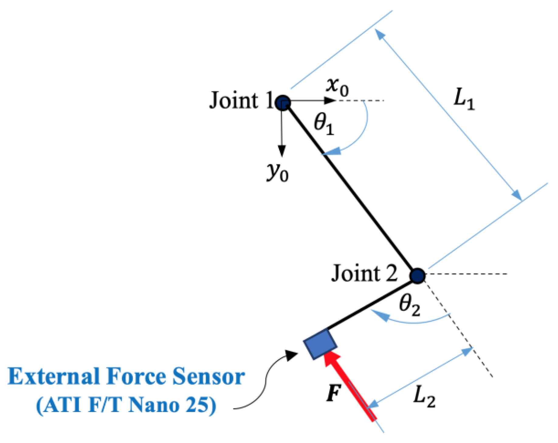
The proposed classifier is designed considering a few inputs/sizes, which are the external joint torques of a 2-DOF manipulator and the force sensor signal, which were estimated in our previous work [14].

(3)

To achieve the high accuracy of the classifier, the proposed PRNN is trained using a conjugate gradient backpropagation algorithm which has a superlinear convergence rate on most problems and is more effective and faster compared with the standard backpropagation. During the training, the main aim and objective is to obtain the smallest or the zero-value cross-entropy. The smaller the cross-entropy, the better the model or the classifier.

(4)

The generalization ability or the effectiveness of the classifier is investigated using different conditions than the training ones.

(5)

The same methodology and work are repeated using a PRNN but is trained in this case by a different training algorithm, which is the Levenberg–Marquardt. The PRNN-LM is compared with the proposed PRNN trained by the conjugate gradient backpropagation algorithm.

(6)

A comparison is presented between our proposed approach (PRNN and PRNN-LM) and the other previous ones to prove its preferability.

The rest of the paper is divided into five sections. Section 2 briefly shows the proposed approach and how it is designed and developed. In Section 3, the experimental work and the generation of the data used, whether for the training, the testing, or the validation processes of the proposed PRNN, are presented. In addition, the ways these processes are carried out are discussed. The results obtained from the three processes (training, testing, and validation) and their discussions are also presented. In Section 4, the repetition of the methodology and the work but using a PRNN trained by Levenberg–Marquardt technique (PRNN-LM) is shown. The comparison between the proposed PRNN and the PRNN-LM is investigated. In addition, this section shows the comparison between the PRNN and PRNN-LM with other previous published works. In Section 5, the conclusion is written and some future works are recommended.

2. Materials and Methods

This section shows how the proposed approach is designed, and the methodology followed in the current paper.

In our previous work [14], an external force sensor was attached at the end-effector of a 2-DOF planar robot, as shown in Figure 1. The KUKA LWR manipulator, which is a collaborative robot, was used for this purpose and was configured as a 2-DOF planar manipulator. Then, an experiment was executed by commanding a sinusoidal motion to the robot joints. During the motion, the human hand made many random collisions at the force sensor. These random collisions mean different magnitudes (low, medium, and high). In other words, the human hand collides with the robot with low, medium, and high forces. In addition, collisions happen at different times during the experiment. In addition, data were collected from the experiment and from the KUKA robot controller (KRC), including the joint positions of the robot, the external joints’ torque, and the force sensor signal.

In [14], a MLFFNN was implemented using the joint positions of the robot as its inputs to estimate the force sensor signal and the external joints torques of the manipulator. The structure of this network is presented in Figure 2a. The MLFFNN was trained by using the Levenberg–Marquardt (LM), and the results proved that the MLFFNN was able to estimate the previously mentioned signals effectively and correctly. The signals estimated by this network are shown in Figure 3. The mean, the standard deviation, the maximum, and the minimum of the absolute value of these signals are presented in

Table 1. The mean, the standard deviation, the maximum, and the minimum of the absolute value of the estimated force sensor signal and the external joints torques of the manipulator, by the MLFFNN.

Parameter	Signal
	External Force Sensor, (N)	External Torque of Joint 1, (Nm)	External Torque of Joint 2, (Nm)
Mean of absolute value	0.4362	0.1830	0.0710
Maximum of absolute value	20.3771	10.7715	3.3552
Minimum of absolute value	4.1624 × 10−6	1.3568 × 10−5	2.2087 × 10−6
Standard deviation of absolute value	1.5284	0.7845	0.2474

. The parameters used with this MLFFNN are presented in

Table 2. The parameters used with the MLFFNN, which was developed to estimate the force sensor signal and the external joint torques.

Parameter	Value
Number of layers	Three layers; input, hidden, and output layers
Number of inputs	Two inputs; the position of joint 1 and of joint 2
Activation function of hidden layer	Tanh (hyperbolic tangent)—hidden layer is nonlinear
Number of hidden neurons	60
Number of outputs	Three outputs; force sensor signal, external torque of joint 1 and of joint 2
Activation function of output layer	Linear
Training algorithm	Levenberg–Marquardt (LM)
Total collected samples	54,229 samples
Number of training samples	46,095 samples
Number of testing samples	5423 samples
Number of validation samples	2711 samples
Software for training process	MATLAB
Processer used for training	Intel(R) Core (TM) i5-8250U [email protected]
Training time	18 min and 26 s
Number of epochs/iterations used	1000
Criterion considered for the training	Obtaining the smallest mean-squared error (MSE). The smaller MSE, the most accurate network in estimation
The MSE obtained	0.06666
Obtained regression from training	R = 0.96618
Obtained regression from testing	R = 0.97292
Obtained regression from validation	R = 0.97582
The average of absolute approximation error resulted from testing process	In case of force sensor signal, 0.1512 Nm In case of external torque of joint 1, 0.0605 Nm In case of external torque of joint 2, 0.0267 Nm
Effectiveness	The results proved that the MLFFNN is efficient and estimates the signals in a correct way

.

In the current work, these estimated force sensor signals and estimated external joint torques are used as inputs for a PRNN, the output of which determines if there is a collision or not, as presented in Figure 2b. Our concentration in the current work is the proposed PRNN. This approach is completed by carrying out the following steps:

(1)

Design of the PRNN based on the estimated signals in [14]. In this step, the structure of the proposed PRNN is presented. The input layer, the hidden layer, and the output layer are investigated in detail. In addition, the number of inputs used is determined.

(2)

Training the designed PRNN using a conjugate gradient backpropagation algorithm. In this stage, parts of the data are used for the training process. The training process is carried out using a scaled conjugate gradient backpropagation algorithm. Many trials and errors are executed to find the best number of hidden neurons, the best activation functions found at the hidden and output layers, and the best number of epochs/iterations, which lead to the high performance of the developed PRNN. The best performance means obtaining very small (about zero value) cross-entropy, which can measure the classification model performance using the probability and error theory. The smaller the cross-entropy, the better the model or the classifier. Therefore, the main aim is to minimize the cross-entropy as small as possible.

(3)

Testing and validating the trained PRNN using other different data than the ones used for training. In this stage, other parts of data which were not used for the train process are used to test and validate the trained PRNN to show its high performance and effectiveness under different conditions and data. If the trained PRNN has the high performance in this step, then it is ready for the classifications. If the trained PRNN does not have high performance, the training process identified in step 2 is repeated until the high performance is produced.

(4)

Studying and investigating the effectiveness of the trained PRNN in classifying the signals. In this stage, the effectiveness in percentage (%) is determined for the PRNN in the training case, validation case, and the testing case. In addition, all the collected data are used together to test the trained PRNN, and its effectiveness (%) is determined.

(5)

The previous steps are repeated but using a PRNN trained by another algorithm, which is the Levenberg–Marquardt (LM) technique. In other words, all the work is repeated by the PRNN-LM. Its effectiveness is calculated in all stages: (1) training, (2) testing, (3) validation, and (4) testing using all data. A comparison is made between the PRNN and the PRNN-LM.

(6)

A comparison is executed between the PRNN and the PRNN-LM classifiers and the other previously published classifiers in terms of the method/approach used, the inputs used during design, the application to real robots, and the effectiveness (%).

All these steps are presented in Figure 4 and discussed and presented in detail in the following section.

3. Results

This section is divided into two subsections. The first subsection shows the experimental work during the design, the training, the validation, and the testing of the proposed PRNN. In the second subsection, the results from these processes are presented.

3.1. Experimental Work

This subsection shows the experiments that are executed and illustrates the design, the training, the validation, and the testing of the proposed PRNN.

As discussed in [14], a sinusoidal motion was executed on the two joints of a 2-DOF planar manipulator, in which an external force sensor (ATI F/T Nano 25) was fixed at the end-effector of this robot. During this experiment, random different collisions were performed by the human operator at the force sensor. Data were collected from KRC and a MLFFNN was designed and trained to estimate the external force sensor signal and the external joints torques of the robot, based only on the joint position sensors that the robot has.

In the current work and based on [14], a PRNN is designed to classify the force sensor signals and to show if there is a collision or not. The NN has many properties, such as its very simple structure [15,16,17], and is easily and efficiently used with different domains, as presented in [5,6,8,18,19,20,21]. In addition, it is characterized by the adaptive and generalization ability and it can approximate linear or nonlinear functions [22,23,24,25]. Using the PRNN, better classification results are obtained when it is used for the classification problems [25,26].

The proposed PRNN, as shown in Figure 5, consists of the following layers:

• The first layer is the input layer, and it contains three inputs: the estimated external force sensor signal and the estimated external torque of joints 1 and 2 of the 2-DOF manipulator. These inputs were obtained from [14].
• The second layer is the nonlinear hidden layer, and it contains an activation function of hyperbolic tangent (tanh) type. After trying many different hidden neurons to achieve a high performance of the designed PRNN, the best number of hidden neurons is 120, as discussed at the end of this section. High performance of NN means achieving very small (about zero value) cross-entropy, which can measure the classification model performance using the probability and error theory, where the more likely or the bigger the probability of something is, the lower the cross-entropy [27]. In other words, cross-entropy is used when adjusting the weights of the model during the training process. The main purpose is minimizing the cross-entropy, and the smaller the cross-entropy the better the model/classifier. A perfect model has a cross-entropy loss of zero value [28].
• The third layer is the nonlinear hidden layer, and it contains an activation function of SoftMax type. The output layer contains two outputs representing two cases: the first one if there is a collision, and the second case if there is not a collision.

It should be noted that the activation function of the hidden and the output layers is selected after trial-and-error experiments until the high performance of the designed PRNN is achieved. As mentioned in point (2), a high performance of PRNN means achieving very small (about zero value) cross-entropy. The smaller the cross-entropy, the better (more accurate) the classifier.

Once the PRNN has been designed, the training, testing, and validation processes are carried out. The training process is executed in MATLAB software and using a scaled conjugate gradient backpropagation algorithm, which is the supervised learning algorithm with superlinear convergence rate in most problems [29,30]. This algorithm is more effective and faster compared with the standard backpropagation [31]. It uses the same concepts of the general optimization strategy, but it chooses the search direction and step size more effectively using information from the second order approximation that is given by the following equation:

$$E\left(w+y\right)\approx E\left(w\right)+E^{\prime }{\left(w\right)}^{T}y+\frac{1}{2}{y}^T{E}^{″}\left(w\right)y$$

(1)

Equation (1) presents the global error function $E\left(w\right)$ in each point $(w+y)$ using the Taylor expansion [31,32]. w is the weight vector. $E\left(w\right)$ depends on all weights and biases that are connected to the NN. Also, $E\left(w\right)$ can be the standard least square function or any other suitable error function.

The collected data that were mentioned in the beginning of this section are 54,229 samples, and they are divided into three groups for training, validating, and testing the proposed PRNN, as presented in in detail in

Table 3. The number of samples that are used for the training, validation, and testing of the proposed PRNN. In addition, the number of samples that contained collisions or not.

Process	Number of Samples	Samples with Collision	Sample without Collision
Training	37,961	1073	36,888
Validation	8134	215	7919
Testing	8134	216	7918

. For showing the effectiveness of the proposed approach, the data that were used for the test and the validation are different from the ones used for the training.

The training of the proposed PRNN happens by trying and carrying out many experiments using different weight initializations and different numbers of hidden neurons until the best performance of the PRNN has been achieved. As mentioned before, the best performance means achieving very small (close to zero value) cross-entropy. Some of these trial-and-error experiments are presented in

Table 4. Some trial-and-error experiments, using different numbers of hidden neurons until the best performance of the designed PRNN has been achieved. The colored cell represents the best case.

	Hidden Neurons
Main parameter to check the performance of the designed PRNN during the training	20	40	60	80	100	120	140	160
Resulting cross-entropy	0.4851	0.3654	0.3281	0.1342	0.0895	0.0697 (the best case)	0.0701	0.0723

.

After the PRNN has been completely trained, the mentioned data in Table 3 are used for testing and validating the trained PRNN to show its effectiveness. The results from these processes are discussed in the next Section 3.2.

3.2. Experimental Results

In this section, the experimental results from the training, testing, and validation of the proposed PRNN are discussed.

During the training stage, after many trial and error experiments, the parameters that achieve the best performance of the PRNN are as follows:

• The number of hidden neurons is 120.
• The number of epochs or iterations is 51. The high performance of the PRNN is achieved after this number of iterations. In other words, once high performance (smallest cross-entropy) has been achieved, the iterations are stopped.
• The smallest obtained cross-entropy is 0.069678.
• The time that consumed for training is 12 s, which is a very short time. However, this time is not very important because the training is carried out offline and the main aim is obtaining a high performance NN in classification.

The resulting results from the training process are presented in Figure 6, Figure 7, Figure 8a and Figure 9a. Figure 6 shows the cross-entropy that resulted from the training. The resulting cross-entropy was 0.069678, which is a very small value and close to the zero value. This means that the proposed PRNN is trained well, and it has high performance and accuracy in classifying the collision and non-collision cases. Figure 7 shows the error histogram, which is the histogram of the errors between the target and the predicted values after training the PRNN. From Figure 7, these error values are close to zero, which indicates that the predicted values are close to the target values; hence the PRNN is trained very well.

ROC (receiver operating characteristic) curves are a very important tool to evaluate the PRNN performance. These curves are widely used for binary classification problems which have two distinct output classes. These curves, resulting from the training process, are shown in Figure 8a. As presented, the ROC curve illustrates the relationship between the true positive rate for the model and the false positive rate. The true positive rate is defined as the rate at which the classifier predicts [positive] for observations that are [positive]. The false positive rate is defined as the rate at which the classifier predicts [positive] for observations that are actually [negative]. The perfect classifier is that which has a true positive rate of 1 and a false positive rate of 0, and this was achieved in our case, as shown in Figure 8a.

The trained PRNN was validated and tested using different data than the training data mentioned in Table 3. This is very important to show the high performance of the trained PRNN using different conditions. The ROC curves resulting from the validation process are shown in Figure 8b. As presented and achieved in this case, the true positive rate is 1 and the false positive rate is 0. This proves that the proposed classifier is perfect and excellent in the validation case. In the testing stage, the resulting ROC curves are shown in Figure 8c. As presented and achieved in this case, the true positive rate is 1 and the false positive rate is 0. This proves that the proposed classifier is perfect and excellent in the testing case. In the final stage, which is shown in Figure 8d, all the collected data (training data + testing data + validation data) are used to test the trained PRNN. In this case, the true positive rate of 1 and the false positive rate of 0 are achieved. This proves that the proposed classifier is perfect and excellent in this case. This discussion proves that the performance of the trained classifier (PRNN) is high when different conditions and data are applied.

The confusion matrix is a very important parameter to show the effectiveness of the method in the classification problem. As shown in Figure 9a, the effectiveness of the PRNN in the training cases is presented. The PRNN can correctly classify 1001 collisions samples out of 1073. Therefore, its effectiveness in classifying the collision cases is 93.3%. The PRNN correctly classified 36,678 non-collisions samples from 36,888. Therefore, its effectiveness in classifying the non-collisions cases is 99.4%. The overall effectiveness of the proposed PRNN in this training stage in classifying both cases is 99.3%, which is considered a very high performance. From this discussion, the proposed PRNN is very well trained and its effectiveness in the training stage is very good.

The trained PRNN is validated and tested using different data than the training data mentioned in Table 3. This is very important to show the high performance of the trained PRNN using different conditions. The effectiveness of the trained PRNN in the validation stage is presented in Figure 9b. The trained PRNN can correctly classify 199 collisions samples from 215. Therefore, its effectiveness in classifying the collision cases is 92.6%. The trained PRNN can correctly classify 7878 non-collisions samples from 7919. Therefore, its effectiveness in classifying the non-collisions cases is 99.5%. The overall effectiveness of the proposed PRNN in this validation stage in classifying both cases is 99.3%, which is a very high performance.

The effectiveness of the trained PRNN in the testing stage is presented in Figure 9c. The trained PRNN can correctly classify 195 collisions samples from 216. Therefore, its effectiveness in classifying the collision cases is 90.3%. The trained PRNN can correctly classify 7870 non-collisions samples from 7918. Therefore, its effectiveness in classifying the non-collisions cases is 99.4%. The overall effectiveness of the proposed PRNN in this testing stage in classifying both cases is 99.2%, which is also a very high performance.

In the final stage, all the collected data (training data + testing data + validation data) are used to test the trained PRNN. The results from this stage are presented in Figure 9d. The trained PRNN can correctly classify 1395 collisions samples from 1504. Therefore, its effectiveness in classifying the collision cases is 92.8%. The trained PRNN can correctly classify 52,426 non-collisions samples from 52,725. Therefore, its effectiveness in classifying the non-collisions cases is 99.4%. The overall effectiveness of the trained PRNN in classifying the collisions and non-collisions cases is 99.2%, which is a very high performance.

From this discussion, we conclude that the trained PRNN can work effectively in classifying the collisions and the non-collisions cases when different conditions and data are applied.

4. Discussion and Comparisons

In this section, the work presented in the previous sections is repeated using a PRNN trained with a different training algorithm, which is the Levenberg–Marquardt (LM). This algorithm is fast and can converge in a short time. In addition, a comparison with other works by previous researchers is carried out.

4.1. PRNN Trained by Levenberg–Marquardt Algorithm (PRNN-LM)

The methodology and work presented in the previous sections is repeated using the PRNN, but in this case trained by Levenberg–Marquardt (LM). It should be noted that, in this case, the number of collision and non-collisions cases in the training, testing, and validation datasets are slightly different compared with the case in the previous sections. This is because MATLAB software divides the data in a random way. This case is presented in

Table 5. The number of samples that are used for the training, validation, and testing of the PRNN-LM. In addition, the number of samples that contain collisions or not.

Process	Number of Samples	Samples with Collisions	Samples without Collisions
Training	37,961	1017	36,944
Validation	8134	227	7909
Testing	8134	242	7892

.

The results (ROC curves and confusion matrix) obtained by the PRNN-LM are presented in Figure 10 and Figure 11.

ROC (receiver operating characteristic) curves are presented in Figure 10. These curves, resulting from the training process, validation process, testing process, and using all collected data are shown, respectively, in Figure 10a–d. As presented and achieved in any of the four cases, the true positive rate is 1 and the false positive rate is 0. This proves that the classifier (PRNN-LM) is perfect and excellent in any case. This discussion proves that the performance of the trained classifier (PRNN-LM) is high whether training data or different conditions and data are applied. These results are approximately the same as the corresponding ones resulting from the PRNN proposed in Section 3.2.

A confusion matrix is a very important parameter to show the effectiveness of the method in the classification problem. As shown in Figure 11a, the effectiveness of the PRNN-LM in the training cases is presented. Its effectiveness in classifying the collision cases is 93.8% and in classifying the non-collisions cases is 99.4%. The overall effectiveness of the developed PRNN-LM in this training stage in classifying both cases is 99.3%, which is considered a very high performance. From this discussion, the developed PRNN-LM is very well trained and its effectiveness in the training stage is very good.

The trained PRNN-LM is validated and tested using different data than the training data mentioned in Table 5. This is a very important step to show the high performance of the trained PRNN-LM using different conditions. The effectiveness of the trained PRNN-LM in the validation stage is presented in Figure 11b. Its effectiveness in classifying the collision cases is 95.0% and in classifying the non-collisions cases is 99.5%. The overall effectiveness of the developed PRNN-LM in this validation stage in classifying both cases is 99.3%, which is a very high performance.

The effectiveness of the trained PRNN-LM in the testing stage is presented in Figure 11c. The effectiveness of the PRNN-LM in classifying the collision cases is 95.2% and in classifying the non-collisions cases is 99.5%. The overall effectiveness of the trained PRNN-LM in this testing stage in classifying both cases is 99.3%, which is also a very high performance.

In the final stage, all the collected data (training data + testing data + validation data) are used to test the trained PRNN-LM. The results from this stage are presented in Figure 11d. Its effectiveness in classifying the collision cases is 94.2% and in classifying the non-collisions cases it is 99.4%. The overall effectiveness of the trained PRNN-LM in classifying the collisions and non-collisions cases is 99.3%, which is a very high performance.

From this discussion, we conclude that the trained PRNN-LM can work effectively in classifying the collisions and the non-collisions cases when different conditions and data are applied. Furthermore, the effectiveness of the trained PRNN-LM is very close to that of the trained PRNN presented in Section 3.2. The overall effectiveness of the trained PRNN presented in previous sections is 99.2%, whereas the overall effectiveness of the trained PRNN-LM is 99.3%.

4.2. Comparison with Other Previous Works

In this subsection, the proposed PRNN and the PRNN-LM are compared with other previous related classifiers. The comparison includes the required inputs for designing the classifier, the application/use, and its overall effectiveness. These classifiers are as follows:

• The first classifier presented by Briquet-Kerestedjian et al. [11] that was based on NN.
• The second classifier proposed by Franzel et al. [12] and based on SVM.
• The third classifier proposed by Al-Haija and Al-Saraireh [13], which was ensemble-based bagged trees (EBT).

The comparison of the required inputs and the applications for the different classifiers are presented in

Table 6. The comparison between the proposed PRNN and PRNN-LM classifiers with other different classifiers in terms of the methods used, the inputs used, and the application to the real robots.

Researcher	Method Used	Inputs Used	Application
Briquet-Kerestedjian et al. [11]	Artificial neural network (NN)	Many inputs, including window of M samples based on actual speeds of the joints and the load joint torques.	The proprietary torque sensor in the robot is required for this approach; therefore, this method is restricted to being used with collaborative robots only.
Franzel et al. [12]	Support vector machine (SVM)	All the sensor readings, such as position and orientation of end-effector, the external torques of each joint, the wrench resulted from an external sensor, and the angles of joints. An external force/torque sensor is required.	As there is no need for any proprietary torque sensor in the robot, the method can be applied to any robot.
Al-Haija and Al-Saraireh [13]	Ensemble-based bagged trees (EBT)	Six inputs, including data from a 140-millisecond time lapse sensor, the motor torque, the external torque, the position, and velocity of the joint.	The proprietary torque sensor in the robot is required for this approach; therefore, this method is restricted to being used with the collaborative robots only.
The current work	PRNN/PRNN-LM	Three inputs, which are the estimated external force sensor signal and the estimated external torques.	As there is no need for any proprietary torque sensor in the robot, the method can be applied to any robot.

. It should be noted that if the classifier design requires a proprietary torque sensor in the robot, then this classifier is restricted to being used only with the collaborative robots which contain the torque and the position sensors. If the classifier design does not require the proprietary torque sensor in the robot, then this classifier can be used with any conventional robots which contain only the position sensor. From Table 6, the proposed PRNN and PRNN-LM, compared with other classifiers, can be used with any robot as their design does not need any proprietary torque sensors in the robot. This proves the generalization of the proposed classifier to any robot. In addition, the inputs used for designing the proposed PRNN and PRNN-LM are fewer, compared with other classifiers. This proves that the proposed classifier is less complex compared with other classifiers.

A comparison of the effectiveness of the different classifiers is presented in Figure 12. As shown in Figure 12, the overall effectiveness of the proposed PRNN and the PRNN-LM in classifying human–robot contacts is better and higher compared with the other classifiers. This proves that the proposed PRNN and PRNN-LM have succeeded in contributing as an effective method for classifying force sensor signals.

5. Conclusions and Future Work

In this paper, a PRNN was developed to classify human robot contacts. Firstly, the PRNN was designed by using the external force sensor signal and the external joint torques of a 2-DOF manipulator, which were estimated in [14] to be its inputs. The output of the proposed PRNN would classify whether there was a collision or not. Secondly, the PRNN was trained by a scaled conjugate gradient backpropagation algorithm using data collected from a sinusoidal joint motion commanded to the robot. The results from this stage achieved the smallest cross-entropy, which was 0.069678 and the effectiveness of the PRNN was 99.3%. These results reveal that the PRNN is trained in an effective way, and it has a high performance in classifying the signals. Thirdly, the trained PRNN was validated and tested using other data and cases from the training ones. The results from this stage prove that the proposed PRNN has a high performance in classifying the collisions and the non-collisions cases, which was 99.2–99.3%. This procedure was repeated using a PRNN, but was trained using a different training method, which was the Levenberg–Marquardt (LM) technique. The results prove that the PRNN-LM is trained well and succeeds in classifying the collisions and the non-collisions cases with high effectiveness (99.3%), close to the corresponding values of the PRNN trained using a scaled conjugate gradient backpropagation algorithm. Finally, the proposed PRNN and PRNN-LM were compared with other, previous classifiers, and the comparison showed that the proposed PRNN and PRNN-LM were the best and had the highest performance.

Future work will apply the proposed approach with a more complex robot, such as a 6- or 7-DOF robot. In addition, identifying which link of the robot has collided will be a consideration. Other different types of neural networks can be investigated, and deep learning as well. Furthermore, analyzing the situations of collisions with obstacles in a more sophisticated way, for example, by identifying the nature of the obstacle encountered, will be considered.

References

1. Ballesteros, J.; Pastor, F.; Gómez-De-Gabriel, J.M.; Gandarias, J.M.; García-Cerezo, A.J.; Urdiales, C. Proprioceptive Estimation of Forces Using Underactuated Fingers for Robot-Initiated pHRI. Sensors 2020, 20, 2863. [Google Scholar] [CrossRef] [PubMed]
2. Sharkawy, A.-N.; Koustoumpardis, P.N. Human–Robot Interaction: A Review and Analysis on Variable Admittance Control, Safety, and Perspectives. Machines 2022, 10, 591. [Google Scholar] [CrossRef]
3. Dimeas, F.; Avendaño-Valencia, L.D.; Aspragathos, N. Human–robot collision detection and identification based on fuzzy and time series modelling. Robotica 2014, 33, 1886–1898. [Google Scholar] [CrossRef]
4. Lu, S.; Chung, J.H.; Velinsky, S.A. Human-Robot Collision Detection and Identification Based on Wrist and Base Force/Torque Sensors. In Proceedings of the 2005 IEEE International Conference on Robotics and Automation, Barcelona, Spain, 18–22 June 2005; pp. 796–801. [Google Scholar]
5. Sharkawy, A.-N.; Aspragathos, N. Human-Robot Collision Detection Based on Neural Networks. Int. J. Mech. Eng. Robot. Res. 2018, 7, 150–157. [Google Scholar] [CrossRef]
6. Sharkawy, A.-N.; Koustoumpardis, P.N.; Aspragathos, N.A. Manipulator Collision Detection and Collided Link Identification Based on Neural Networks. In Advances in Service and Industrial Robotics. RAAD 2018. Mechanisms and Machine Science; Nikos, A., Panagiotis, K., Vassilis, M., Eds.; Springer: Cham, Switzerland, 2018; pp. 3–12. [Google Scholar] [CrossRef]
7. Sharkawy, A.-N.; Koustoumpardis, P.N.; Aspragathos, N. Human–robot collisions detection for safe human–robot interaction using one multi-input–output neural network. Soft Comput. 2020, 24, 6687–6719. [Google Scholar] [CrossRef]
8. Sharkawy, A.-N.; Koustoumpardis, P.N.; Aspragathos, N. Neural Network Design for Manipulator Collision Detection Based Only on the Joint Position Sensors. Robotica 2020, 38, 1737–1755. [Google Scholar] [CrossRef]
9. Sharkawy, A.-N.; Ali, M.M. NARX Neural Network for Safe Human–Robot Collaboration Using Only Joint Position Sensor. Logistics 2022, 6, 75. [Google Scholar] [CrossRef]
10. Mahmoud, K.H.; Sharkawy, A.-N.; Abdel-Jaber, G.T. Development of safety method for a 3-DOF industrial robot based on recurrent neural network. J. Eng. Appl. Sci. 2023, 70, 1–20. [Google Scholar] [CrossRef]
11. Briquet-Kerestedjian, N.; Wahrburg, A.; Grossard, M.; Makarov, M.; Rodriguez-Ayerbe, P. Using Neural Networks for Classifying Human-Robot Contact Situations. In Proceedings of the 2019 18th European Control Conference, ECC 2019, EUCA, Naples, Italy, 25–28 June 2019; pp. 3279–3285. [Google Scholar] [CrossRef]
12. Franzel, F.; Eiband, T.; Lee, D. Detection of Collaboration and Collision Events during Contact Task Execution. In Proceedings of the IEEE-RAS International Conference on Humanoid Robots, Munich, Germany, 19–21 July 2021; pp. 376–383. [Google Scholar] [CrossRef]
13. Abu Al-Haija, Q.; Al-Saraireh, J. Asymmetric Identification Model for Human-Robot Contacts via Supervised Learning. Symmetry 2022, 14, 591. [Google Scholar] [CrossRef]
14. Sharkawy, A.; Mousa, H.M. Signals estimation of force sensor attached at manipulator end-effector based on artificial neural network. In Handbook of Nanosensors: Materials and Technological Applications; Ali, G.A.M., Chong, K.F., Makhlouf, A.S.H., Eds.; Springer Nature: Berlin/Heidelberg, Germany, 2023; pp. 1–25. [Google Scholar]
15. Schmidhuber, J. Deep Learning in Neural Networks: An Overview. Neural Netw. 2015, 61, 85–117. [Google Scholar] [CrossRef] [PubMed]
16. Haykin, S. Neural Networks and Learning Machines, 3rd ed.; Pearson: London, UK, 2009. [Google Scholar]
17. Sharkawy, A.-N. Principle of Neural Network and its Main Types: Review. J. Adv. Appl. Comput. Math. 2020, 7, 8–19. [Google Scholar] [CrossRef]
18. Chen, S.-C.; Lin, S.-W.; Tseng, T.-Y.; Lin, H.-C. Optimization of Back-Propagation Network Using Simulated Annealing Approach. In Proceedings of the 2006 IEEE International Conference on Systems, Man and Cybernetics, Taipei, Taiwan, 8–11 October 2006; pp. 2819–2824. [Google Scholar] [CrossRef]
19. Sassi, M.A.; Otis, M.J.-D.; Campeau-Lecours, A. Active stability observer using artificial neural network for intuitive physical human–robot interaction. Int. J. Adv. Robot. Syst. 2017, 14, 1–16. [Google Scholar] [CrossRef]
20. De Momi, E.; Kranendonk, L.; Valenti, M.; Enayati, N.; Ferrigno, G. A Neural Network-Based Approach for Trajectory Planning in Robot–Human Handover Tasks. Front. Robot. AI 2016, 3, 1–10. [Google Scholar] [CrossRef]
21. Sharkawy, A.-N.; Koustoumpardis, P.N.; Aspragathos, N. A recurrent neural network for variable admittance control in human–robot cooperation: Simultaneously and online adjustment of the virtual damping and Inertia parameters. Int. J. Intell. Robot. Appl. 2020, 4, 441–464. [Google Scholar] [CrossRef]
22. Rad, A.B.; Bui, T.W.; Li, Y.; Wong, Y.K. A new on-line PID tuning method using neural networks. In Proceedings of the IFAC Digital Control: Past, Present and Future of PID Control, Terrassa, Spain, 5–7 April 2000; Volume 33, pp. 443–448. [Google Scholar]
23. Elbelady, S.A.; Fawaz, H.E.; Aziz, A.M.A. Online Self Tuning PID Control Using Neural Network for Tracking Control of a Pneumatic Cylinder Using Pulse Width Modulation Piloted Digital Valves. Int. J. Mech. Mechatron. Eng. IJMME-IJENS 2016, 16, 123–136. [Google Scholar]
24. Hernández-Alvarado, R.; García-Valdovinos, L.G.; Salgado-Jiménez, T.; Gómez-Espinosa, A.; Fonseca-Navarro, F. Neural Network-Based Self-Tuning PID Control for Underwater Vehicles. Sensors 2016, 16, 1429. [Google Scholar] [CrossRef]
25. Xie, T.; Yu, H.; Wilamowski, B. Comparison between Traditional Neural Networks and Radial Basis Function Networks. In Proceedings of the 2011 IEEE International Symposium on Industrial Electronics, Gdansk, Poland, 27–30 June 2011; pp. 1194–1199. [Google Scholar]
26. Jeatrakul, P.; Wong, K.W. Comparing the performance of different neural networks for binary classification problems. In Proceedings of the 2009 Eighth International Symposium on Natural Language Processing, Bangkok, Thailand, 20–22 October 2009; pp. 111–115. [Google Scholar] [CrossRef]
27. Bhardwaj, A. What is Cross Entropy? Published in Towards Data Science. 2020. Available online: https://towardsdatascience.com/what-is-cross-entropy-3bdb04c13616 (accessed on 3 November 2020).
28. Koech, K.E. Cross-Entropy Loss Function. Published in Towards Data Science. 2020. Available online: https://towardsdatascience.com/cross-entropy-loss-function-f38c4ec8643e (accessed on 2 October 2020).
29. Møller, M.F. A scaled conjugate gradient algorithm for fast supervised learning. Neural Netw. 1993, 6, 525–533. [Google Scholar] [CrossRef]
30. Nayak, S. Scaled Conjugate Gradient Backpropagation Algorithm for Selection of Industrial Robots. Int. J. Comput. Appl. 2017, 6, 92–101. [Google Scholar] [CrossRef]
31. Gill, P.E.; Murray, W.; Wright, M.H. Practical Optimization; Emerald Group Publishing Limited: Bingley, UK, 1982. [Google Scholar]
32. Hestenes, M.R. Conjugate Direction Methods in Optimization; Springer: New York, NY, USA, 1980. [Google Scholar] [CrossRef]
Figure 1. The experimental setup by attaching an external force sensor at the end-effector of a 2-DOF planar manipulator.
Robotics 12 00124 g001
Figure 2. The proposed methodology in the current work. (a) An MLFFNN is first used to estimate the external force sensor signal and the external joint torques of the robot, as presented in the previous work. (b) A PRNN is designed, using the estimated force sensor signal and the estimated external joints torques as its inputs, and the output is whether there is a collision or not. In this Figure, 1 is the bias.
Robotics 12 00124 g002
Figure 3. The estimated signals from the MLFFNN. (a) The external force sensor signal, (b) the external torque of joint 1 of the 2-DOF manipulator, and (c) the external torque of joint 2 of the 2-DOF manipulator. These signals are the inputs of the newly developed PRNN.
Robotics 12 00124 g003
Figure 4. The steps followed in the current work start from collecting the data and until readiness for classifying the force sensor signals.
Robotics 12 00124 g004
Figure 5. The design of the proposed PRNN. The inputs are three, which are the estimated external force sensor signal and the estimated external torque of joint 1 and 2 of the 2-DOF robot that were obtained from [14]. The outputs are two cases, which are when there is a collision and when there is not a collision. In Figure, 3 represents the number of inputs, 120 represents the number of hidden neurons, and 2 represents the number of outputs.
Robotics 12 00124 g005
Figure 6. The cross-entropy resulting during the training process of the PRNN. The curves representing the training, validation, and testing cases coincide together, as in the lower Figure. For more illustration, the upper Figure shows the curves of the training and validation cases.
Robotics 12 00124 g006
Figure 7. The error histogram resulting from the PRNN training.
Robotics 12 00124 g007
Figure 8. The receiver operating characteristic (ROC) curves resulting from (a) the training process, (b) the validation process, (c) the test process, and (d) using all the collected data for testing the trained PRNN.
Robotics 12 00124 g008
Figure 9. The effectiveness of the proposed PRNN in classifying the collisions cases and the non-collision cases from (a) the training process, (b) the validation process, (c) the test process, and (d) using all the collected data for testing the trained PRNN; 1 represents the collision cases and 2 represents the non-collisions cases. The cells with green color represent correctly classified cases, whereas the cells with red color represent the misclassified cases.
Robotics 12 00124 g009
Figure 10. The receiver operating characteristic (ROC) curves resulting from (a) the training process, (b) the validation process, (c) the test process, and (d) using all the collected data for testing the trained the PRNN-LM.
Robotics 12 00124 g010
Figure 11. The effectiveness of the proposed PRNN-LM in classifying the collisions cases and the non-collisions cases from (a) the training process, (b) the validation process, (c) the test process, and (d) using all the collected data for testing the trained PRNN-LM; 1 represents the collisions cases and 2 represents the non-collisions cases. The cells with green color represent correctly classified cases, whereas the cells with red color represent the misclassified cases.
Robotics 12 00124 g011
Figure 12. Comparison between the effectiveness (%) of the proposed PRNN and the PRNN-LM with other previous different classifiers.
Robotics 12 00124 g012