The next paragraphs describe the details of each skill, providing further details of the different calculations and step sequences.
6.2.1. Workbench Configuration Skill
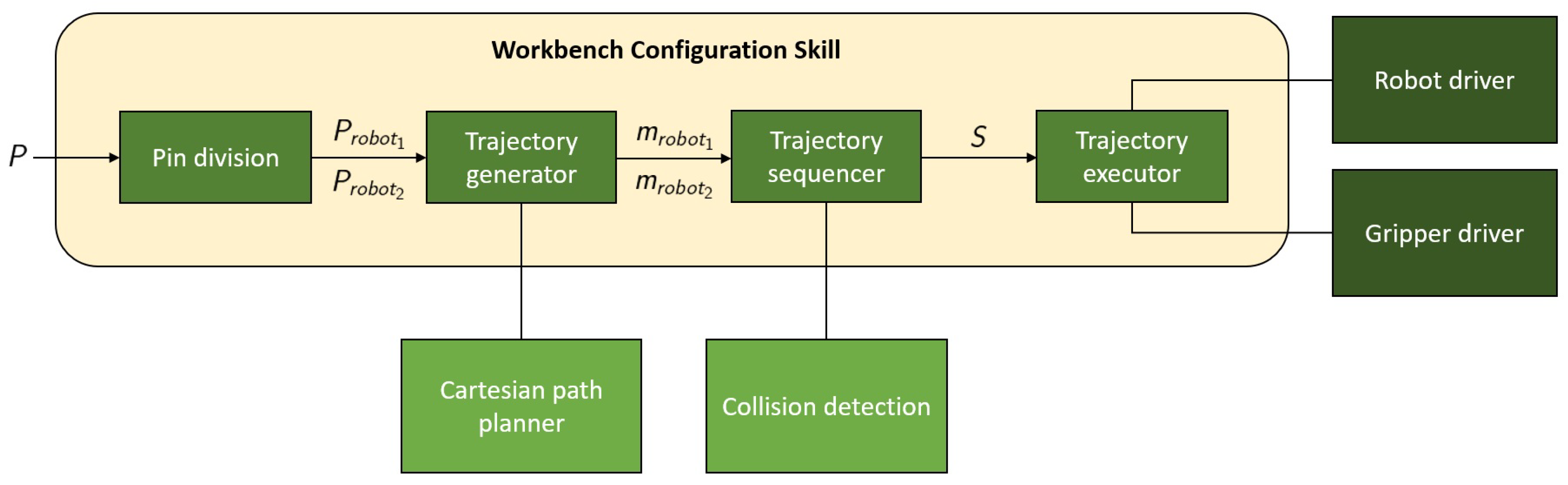
The Workbench Configuration Skill receives the pin position set P as input. Initially, it determines which robot places each pin to divide and speed up the task. Afterwards, all the pin placement trajectories are calculated, determining if it is possible to execute them in parallel or if it would cause any collision between the robots. Finally, all the robot movements are executed and the grippers are activated as determined in the plan.
Specifically, the workbench configuration workflow, depicted in
Figure 8, follows several key steps:
Initially, the Pin division step divides the pins to be placed, assigning them to the most appropriate robot arm.
The second step is the Trajectory generation, where the module calculates the robot trajectories for the pin grasping and placing manoeuvres.
In the fourth step the Trajectory sequencer defines the final trajectory sequence, checking if both robots can execute the movements in parallel to speed up the process.
Finally, the Trajectory executor manages all these trajectories, operating both robots and grippers as defined in the plan.
The next lines provide further details on these four steps of the workflow and the calculation of the different modules.
Initially, the
Pin division step divides the pin position set
P into two disjoint sets
and
where each pin
of the set
P is assigned to the nearest robot
based on the transformations between both robots and each pin position of the set
PThe
Trajectory generator uses these two subsets
and
to calculate the trajectories for the pin grasping and pin placement. Specifically, the maneuver
m of grasping and positioning of the pin
i for each robot’s subset
and
is defined by a set of trajectories
where
and
describe the trajectory from the safe pose to each robot’s pin feeder,
and
define the trajectory from the pin feeder to the pin placement pose on the CAD drawing and
describe the trajectory back to the safe position from the pin pose on the CAD drawing.
All these manoeuvres represent a sequence of trajectories for each robot
where both
and
define a specific sequence
S of robot trajectories for picking and placing pins.
Finally, the
Trajectory sequencer checks if the defined trajectories can be executed in parallel without any collision or if they must be executed in a row to avoid any contact between the robots during the manoeuvres. Specifically, the collision check module will determine if maneuvers
and
can be executed simultaneously
or they must be placed one behind the other
in the complete manoeuvre sequence.
After the complete planning, the Trajectory executor receives the sequence S and executes all the planned trajectories in the provided order, moving the robots and managing the grippers as defined in the complete plan.
6.2.2. Routing Skill
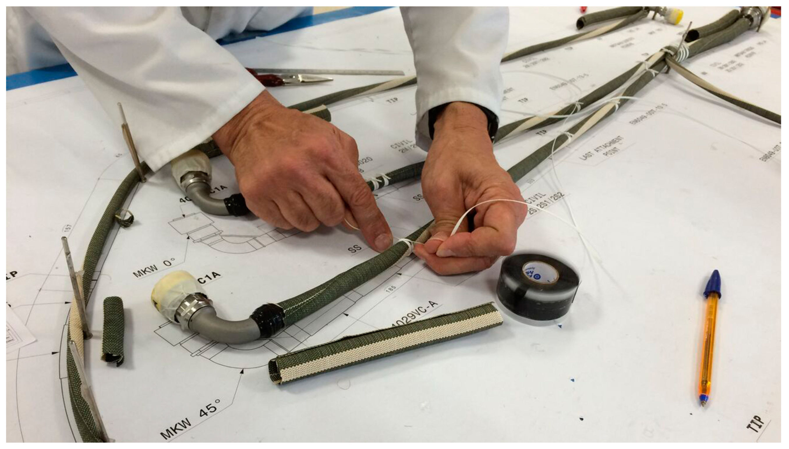
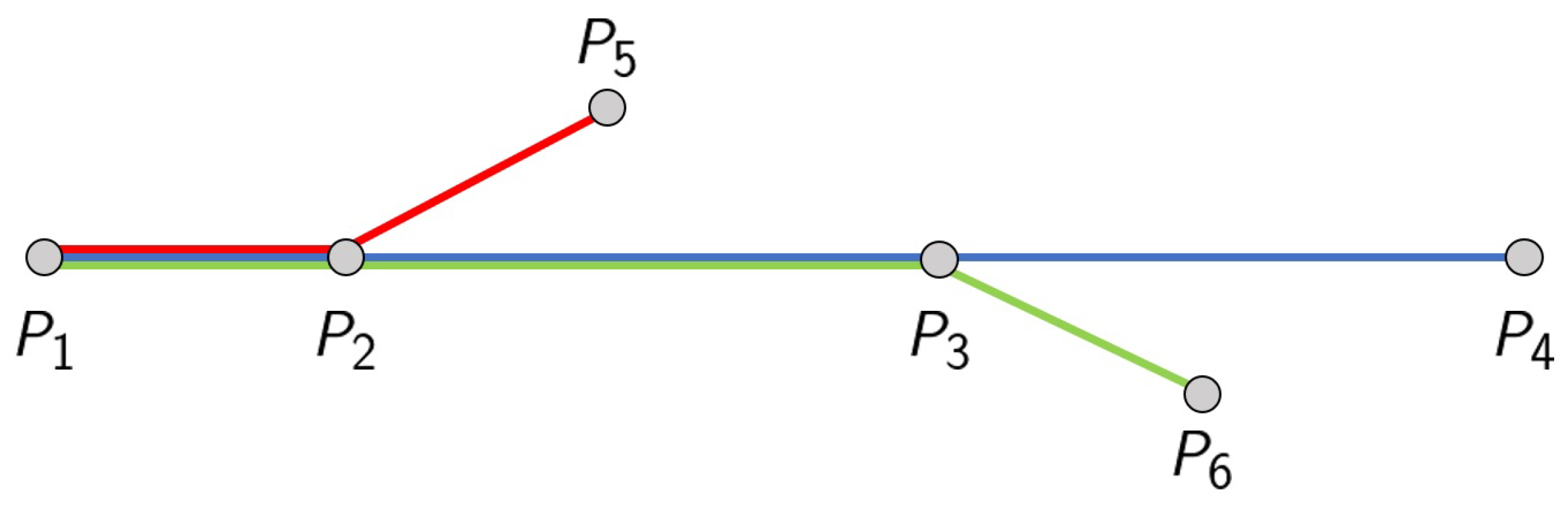
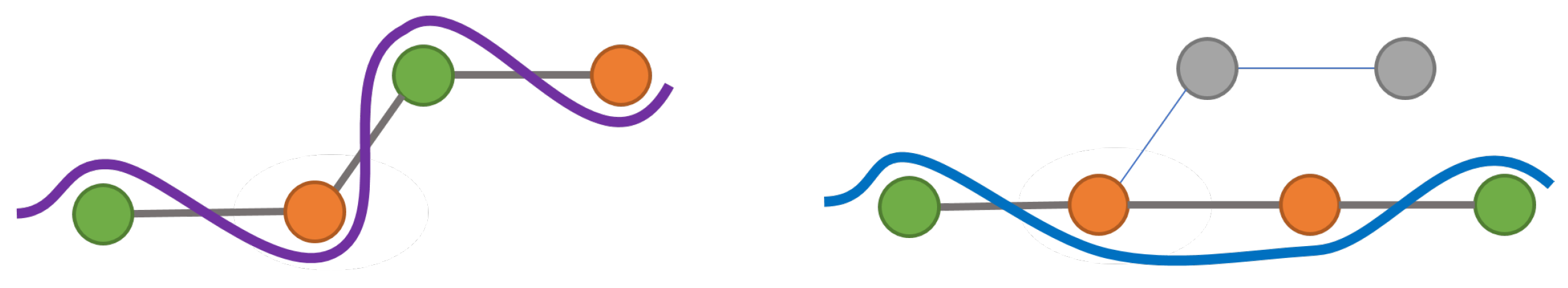
An important characteristic of the routing task is that operators follow a strategy in the process. During the routing, if curvature is found in the path, operators guide the wire through the external side of the pin. In the straight segments of the path, operators select arbitrarily the pin side. Additionally, at the endpoints, operators change the pin side to secure the wire. Therefore, a routing pathway will include some pins where operators are forced to select one specific side of the pins and some others where they can choose freely, as illustrated in the examples of
Figure 9. The
Routing Skill incorporates this strategy into the robots’ workflow.
Specifically, the Routing Skill is in charge of defining, planning, and executing the routing trajectory of a single cable. The module receives a set P of already positioned pins, as well as the path containing the set of pins that compose the routing pathway of cable i defined in the Offline Programming Framework.
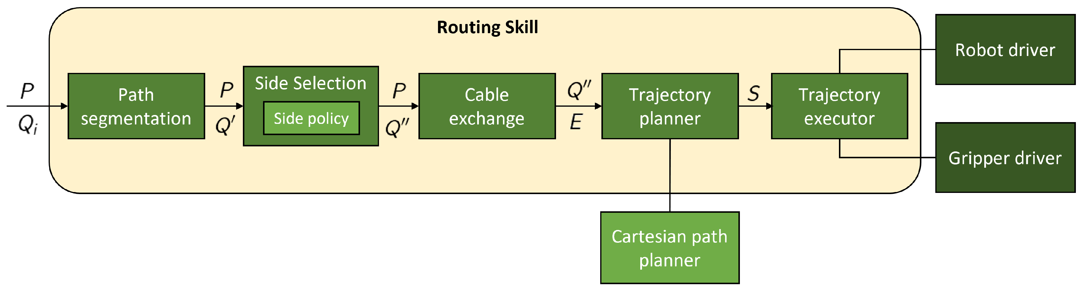
The routing workflow, depicted in
Figure 10, follows several key steps:
Initially, the path is subjected to a Path segmentation process, dividing the routing path into distinct segments assigned to the most appropriate robot arm.
The second step is the Side selection, where the module defines the pin side that the path will follow to meet the routing strategy described above.
The third step is the Cable exchange, where the most suitable cable exchange positions are estimated when both robots need to hand over the wire.
In the fourth step the Trajectory planner calculates the robot trajectories of the previously calculated routing paths and cable exchange manoeuvres.
Finally, the Trajectory executor manages all these trajectories, handling both robots and grippers as defined in the plan.
The next lines provide further information on these five steps of the workflow.
Initially, the
Path segmentation step divides the complete pathway
, assigning each segment to the most appropriate robot. Specifically, the routing pathway positions in
are divided into
N segments
where
The module assigns each pin position to the nearest robot. In the case of a cable where all its pins reside within a single arm’s reach, the whole set of points is assigned to one segment . Otherwise, if a cable exchange is required between robots at any point in the complete path, that segment concludes. As a result, the cable’s path is divided into N segments where N can not be higher than the number of pins defining the routing path.
After the segmentation, the
Side selection step modifies these original segments by including additional manoeuvres to ensure that the robots do not collide with the pins and follow the correct routing strategy. Therefore, this step modifies the segment set
, generating a new segment set
where the points
are modified to comply with the routing strategy. Specifically,
is defined as
where
is a set of points of the same size as
where the positions are modified to include the routing strategy manoeuvres.
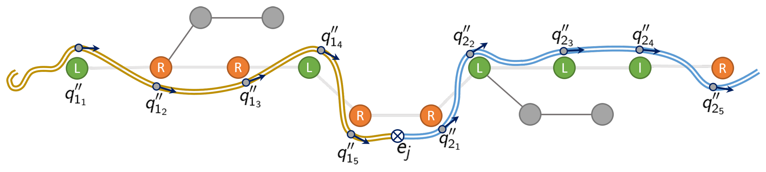
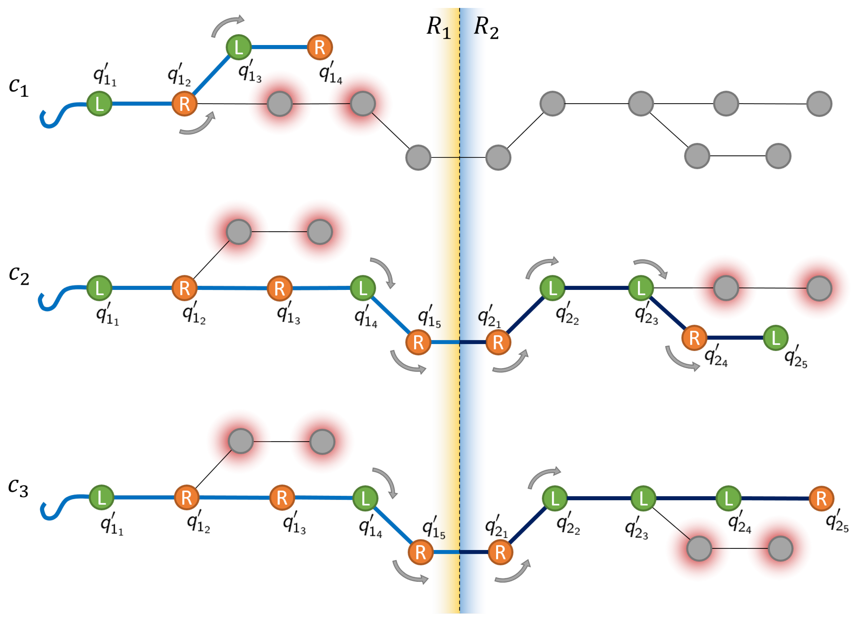
In the context of the routing pathway evaluation,
Figure 11 provides a graphical representation of the routing strategy for three different cables, listed in descending order. The first cable, shown in the first row and labelled as
, illustrates a case where a cable with a shorter path can be routed in its entirety by a single robotic arm. Conversely, the second and third cables, labelled as
and
respectively, present more complex routing cases, as their paths are divided into two segments by the line that intersects the workspace of robot
and robot
.
To achieve the required shape, the cable must pass through either the left or right side of the various pins on its path, denoted in
Figure 11 by
L or
R respectively. Determining the proper go-through side for every pin is a key aspect of ensuring that the cable maintains the desired shape and avoids unexpected snaps or movements. Therefore, for any pin
i, its side
is expected as such
where
represents the chosen side (left or right) for pin
i.
A side convention is used, which establishes that the cable must pass through the external side of the pin at each bend or turning point. The external side policy ensures that the condition is met by calculating the curvature
as
where
corresponds to the Y component of the relative transformation between positions
and
, which is extracted from the homogeneous matrix
calculated as
where
and
define the homogeneous transformation of path position
and
respectively.
Additionally,
Figure 11 shows that for any pin located in straight sections of the path, there is no concern for curvature. Instead, the collision risk is evaluated. The collision policy assesses the chance of the robot, its gripper, or the grasped cable colliding with surrounding pins. The idea is to choose the side with lower collision risk (fewer pins in the area). This collision risk is estimated for every pin in the path, and for each side. For example, for a pin
, the cost of the left side
L is calculated by adding the cost of all pins
located within that side, while the cost of each individual pin
depends on its distance to the current pin
where
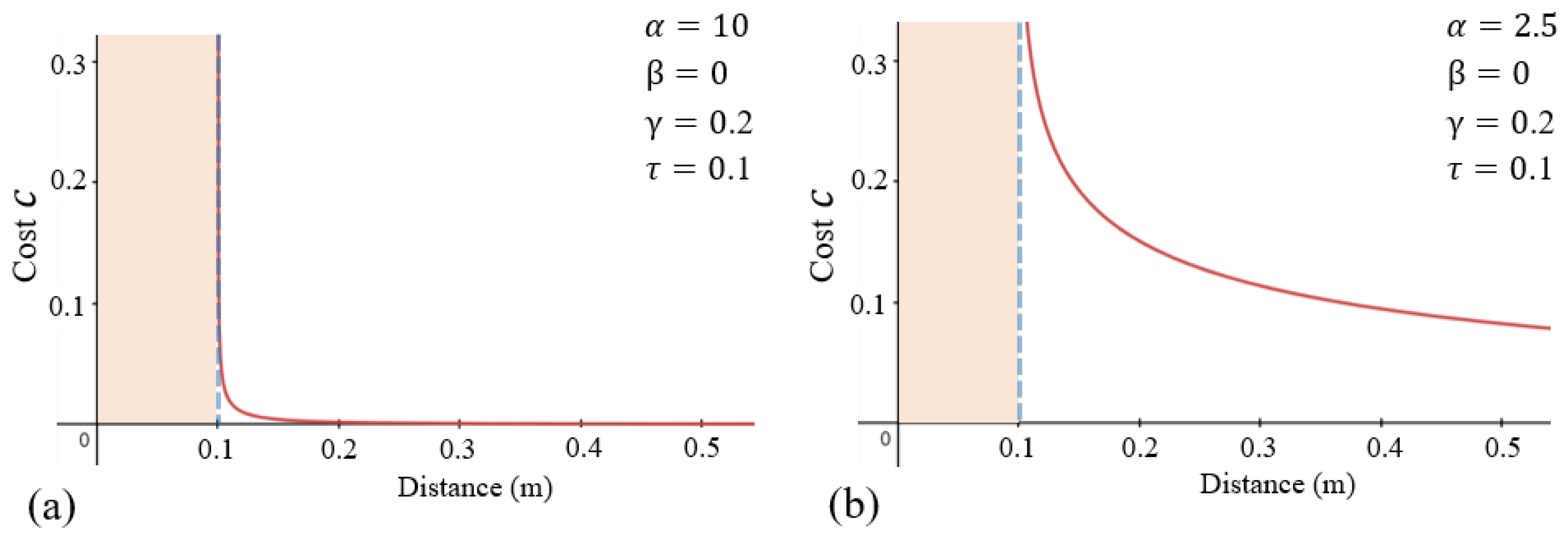
Therefore, the total cost per side is defined as
where parameters
,
, and the exponent
control the shape of the decay curve, while
and
represent the total number of pins on the left side and on the right side, respectively. Additionally,
stands for a previously defined safe threshold that can be adjusted. The decay curve and its shape determine the collision cost of any given pin
based on its relative distance to the current pin
. As shown in
Figure 12, subfigure (a) depicts a cost curve that drastically decays past the safety threshold, reducing concern over pins outside the safety threshold. This curve is particularly well-suited for layouts with low concentrations of pins. On the contrary, subfigure (b) shows a gradually declining curve, which might be preferable for layouts with higher pin densities or more cramped conditions, as it allows further consideration over pins located beyond the threshold.
Considering both the external side convention and, in the case of straight sections, the collision risk, the optimal go-through side is determined by the following conditions
where
is used as a variable representing the curvature of the path.
The obtained side
is then used to define the point through which the cable passes. It is defined as
where
denotes the selected side sign. This value is used in
where
represents the translation vector, defined by the side factor
multiplied by the safety threshold
. Therefore, following the routing strategy, a modified nominal point
can be obtained from the original
by means of
where the +homogeneous transformation
is defined as
where
represents the nominal pin position and
depict the rotation matrix aligning the
Z angle to face the next pin.
The third step of the routing workflow is the Cable exchange. Whenever a segment ends and another begins, a cable exchange should take place, an exchange where one robot hands over the cable to the other by carefully placing it on the table. To this end, a feasible position is required where the cable can be laid down and picked up by the second robot without disturbances. In the case of the end of the route, the exchange point is considered the final cable tip position.
Specifically, the
Cable exchange module receives the set of segments
and generates the new set
E which includes the exchange points when required. Therefore,
E is defined as
where each point
defines the exchange point of segment
j.
As shown in
Figure 13, the ideal exchange point
is located between segments, represented as ⨂. It is determined by the intersection of the intermediate plane between the two robots and the current path’s segment
. The intersection point
is defined as
where
n is the normal vector of the intermediate plane,
p represents the vector of the routing segment and
is the point residing in the intermediate plane. After determining the ideal exchange point, to avoid any possible clash with nearby pins or already placed cables, a radiating search is performed to find the nearest valid place to rest the cable. This involves an iterative search process, which starts within the exchange point and radiates out checking nearby positions until a valid point is found.
After determining the passing sides and exchange positions, the
Trajectory planner uses the set of segments
and the set of exchange points
E to generate the routing robot trajectories
S. The trajectory planning is also conducted by segments, each involving the planning of all manoeuvres: Cable grasp, routing across the pins while drawing the desired shape for each segment, and finally a retreat manoeuvre to ensure that the workspace is free for the other robot. Therefore, trajectory set
S is defined by
where
,
, and
define the grasping, routing and retreat maneuvers of segment
j.
After the trajectory planning, the Trajectory executor receives the sequence S and executes all the planned trajectories, managing the robots and grippers as defined in the sequence.


