Article

A Novel Error Sensitivity Analysis Method for a Parallel Spindle Head

1
State Key Laboratory of Tribology, Department of Mechanical Engineering, Tsinghua University, Beijing 100084, China
2
Beijing Key Laboratory of Precision/Ultra-Precision Manufacturing Equipment and Control, Beijing 100084, China
*
Author to whom correspondence should be addressed.
Robotics 2023, 12(5), 129; https://doi.org/10.3390/robotics12050129
Submission received: 13 August 2023 / Revised: 4 September 2023 / Accepted: 10 September 2023 / Published: 11 September 2023
(This article belongs to the Special Issue Kinematics and Robot Design VI, KaRD2023)

Abstract

:
Geometric errors are the main factors affecting the output accuracy of the parallel spindle head, and it is necessary to perform a sensitivity analysis to extract the critical geometric errors. The traditional sensitivity analysis method analyzes the output position and orientation errors independently, defining multiple sensitivity indices and making it difficult to determine critical geometric errors. In this paper, we propose sensitivity indices that can comprehensively consider position and orientation errors. First, the configuration of the hybrid machine tool is introduced, and the TCP position error model is derived. Then, the tool radius and the effective cutting length are introduced, and the sensitivity indices are defined. After that, the sensitivity analysis of the 3-DOF parallel spindle head is performed using the proposed sensitivity indices, and six critical geometric errors are extracted. The machining accuracy of the parallel spindle head can be greatly improved by improving the critical geometric errors. The proposed sensitivity analysis method can provide important guidance for machine tool accuracy design.

1. Introduction

Due to the large demand for complex parts, five-axis machine tools are widely used in production practice [1,2]. Among them, hybrid machine tools combine the advantages of high stiffness, low inertia, and high flexibility of the parallel mechanism and the advantages of a large working space for the series mechanism, which have higher machining efficiency compared with traditional five-axis machines and become ideal configurations for aerospace machining [3,4,5].
Accuracy performance is the main index that evaluates the effectiveness of machining, fabrication, and deburring [6,7,8]. The factors affecting the accuracy of machine tools mainly include geometric errors, thermal errors, load-induced structural deformation errors, and servo errors [9,10]. Among them, geometric error is the main error source, accounting for 40–50% of the total error source [11]. For the hybrid machine tool, due to the existence of a large number of limbs and passive joints, the geometric error of the parallel spindle head is the main factor causing the error [12,13]. Therefore, how to improve the geometric accuracy of the parallel spindle head is the key to ensuring the machining accuracy of the hybrid machine tool.
There are two ways to improve the geometric accuracy of parallel spindle heads: precision design and error compensation [14]. Precision design refers to the elimination of possible error sources in the design, manufacturing, and assembly of machine tools by optimizing materials and structures and ensuring assembly quality [15]. The corresponding error compensation technology, mainly through the establishment of an error model and the measurement and identification of each error parameter, compensates the identified error in real time in practical application to improve the accuracy [16,17]. Whether it is a precision design or error compensation, it is important to evaluate the error parameters. Therefore, establishing the relationship between the error parameters and output errors and performing a sensitivity analysis is the key to accuracy improvement. By comparing the sensitivity indices, the structural errors that have a greater impact on machining accuracy can be extracted so that more attention can be paid to them in the process of design, manufacture, assembly, and use.
Error modeling is used to establish the relationship between the geometric error parameters and the output errors [18]. According to the different methods of mathematical description of joint motion, the error modeling methods can be divided into the matrix method [19,20], the screw method [21,22], and the vector method [23,24]. The matrix method, taking the D-H method as an example, mainly establishes a local coordinate system in each component, describes the motion relationship of adjacent components through the homogeneous transformation matrix, and constructs the relationship between each error parameter and the output error with the matrix product, differentiation, and other operations. However, the presence of multiple limbs and passive joints of parallel mechanisms makes the matrix method very difficult to model. The screw method represents the instantaneous motion of the moving and rotating joints by means of screws and then obtains the motion of the moving and rotating joints by integrating the screws. However, the complexity of the derivation, the lack of practical physical meaning of the error parameters, and the severe parameter redundancy greatly limit its use in error modeling of parallel mechanisms. The vector method is used to construct closed-loop vector equations and then differentiate each parameter and simplify them by vector operations to obtain the transfer relationship between the error parameters and the output error. The vector expression form is intuitive, and the physical meaning is clear, which is very suitable for the error modeling of parallel mechanisms with closed-loop structural features, and the closed-loop vector method is used for geometric error modeling in this paper.
Error sensitivity refers to the influence of each geometric error parameter on the output error, and sensitivity analysis can guide the extraction of the critical geometric error of the mechanism [25] and provide a basis for the optimization of mechanical performance [26,27]. The sensitivity analysis of the geometric error is mainly divided into two types: local sensitivity analysis (LSA) and global sensitivity analysis (GSA) [28]. LSA is mainly used to analyze the effect of geometric error on the output error when the tool is located at a particular pose, while GSA analyzes the average effect of error parameters on the output error in the entire workspace. Patel [29] analyzed the error sensitivity of the Hexapod parallel machine tool by approximate linear error mapping. Fan [30] analyzed the sensitivity of the 3-PRS parallel mechanism and identified its critical errors using the partial differential method based on the error transform vector. Defining the sensitivity index is the key to sensitivity analysis. Since the output error contains both position and orientation errors, multiple sensitivity indices exist when the elements in the output error vector are analyzed independently in the traditional sensitivity analysis method. And the position and orientation errors are inhomogeneous, making it difficult to compare multiple error sensitivity indices and thus difficult to identify critical geometric errors. Jiang [31] and Du [32] used the Monte Carlo algorithm to analyze the sensitivity of the 3-DOF parallel spindle head as well as the 2UPR-RPU over-constrained parallel manipulator, respectively, but they constructed two sensitivity indices for output position and orientation, respectively, which are still difficult to compare. To solve this problem, the influence of geometric error on the tool orientation error is ignored, and only the tool center point (TCP) position error is considered to construct the error sensitivity index in Refs. [33,34,35], which can reduce the number of sensitivity indices and facilitate the comparison. However, the tool orientation error also has a large impact on the machining accuracy, and ignoring the orientation error leads to incomplete error sensitivity analysis. Li [36] proposed a sensitivity analysis method for the position and orientation errors by introducing the average cutting length, but the method actually converts the orientation error into the positional error of a point on the tool, whereas in the actual cutting process, the actual cutting is performed not just at a point on the tool, and thus the method cannot fully reflect the impact on machining accuracy. In addition, most of the sensitivity analysis methods are based on the error values of position and orientation errors or the TCP position error modulus to model the sensitivity indices; however, when the tool is in different poses, the same position error values bring different impacts on machining accuracy, and the traditional methods cannot consider the impacts of the error values on the machining accuracy in different pose, which results in an incomplete analysis of the error sensitivity. In summary, it is necessary to propose a single sensitivity index that comprehensively considers position and orientation errors and can directly evaluate the effect of geometric errors on machining accuracy at each pose.
In this paper, a new method of sensitivity analysis is proposed. By introducing the tool radius and effective cutting length, a sensitivity index that can comprehensively consider the position and orientation errors is defined, which solves the problem that the traditional sensitivity indexes are difficult to compare and cannot fully reflect the machining accuracy.
Following this section, in Section 2, the configuration of the hybrid machine tool is introduced, and the TCP position error model is derived using the closed-loop vector method. In Section 3 the error sensitivity indices are defined. In Section 4, the error sensitivity of the 3-DOF parallel spindle head is analyzed using the proposed sensitivity indices, and the simulation results are discussed. Finally, the conclusion of this paper is given.

2. Configuration and Error Modeling
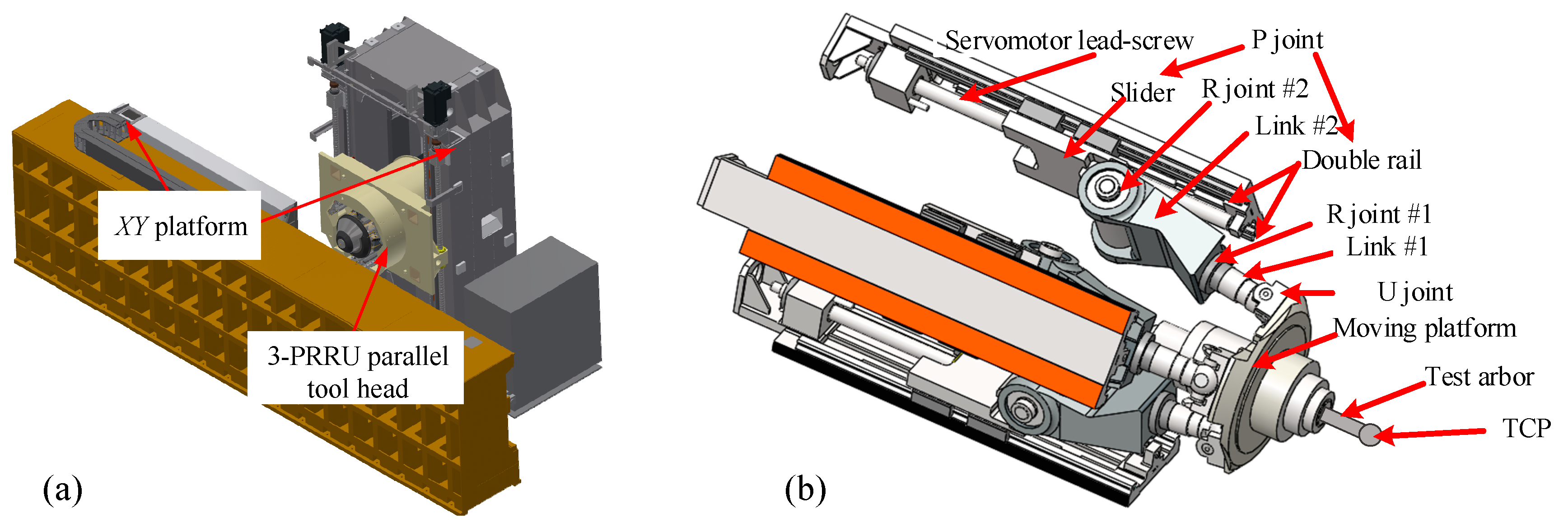
2.1. Configuration

Figure 1 shows the five-axis hybrid machine tool studied in this paper, which consists of a working platform and a 3-DOF parallel spindle head mounted on a column. A base platform and a moving platform are connected by three identical PRRU limbs to form the 3-DOF parallel spindle head, as shown in Figure 1b. Here P, R, and U denote prismatic, revolute, and universal joints, respectively. The three P joints are actuated joints. The parallel spindle head can realize Z-direction movement and rotation around the X and Y axes and cooperate with the XY platform to realize 5-DOF motion. The XY platform is essentially two perpendicular linear axes with a very simple structure, making it easy to compensate for geometric errors. The 3-DOF parallel spindle head has a complex structure with a large number of limbs and passive joints, resulting in a large manufacturing and assembly error. And the nonlinear motion characteristics of the parallel spindle head lead to difficulties in compensating for its geometric errors. Therefore, the geometric error of the 3-DOF parallel spindle head is the main source of geometric error in the five-axis hybrid machine tool. This paper mainly analyzes the error sensitivity of this 3-DOF parallel spindle head.

2.2. TCP Position Error Modeling

In kinematic studies, the 3-PRRU structure can be simplified to a 3-PRS mechanism. For each limb, its closed-loop vector equation is constructed.
H + R TT R i a i = R i b i + R i R B i q i + R i R B i R C i l i
where ai, bi, and li are shown in Figure 2. H = [x y z]T denotes the vector OO’, qi represents the drive vector, Ri represents the rotation matrix of each limb, and RBi and RCi denote the rotation matrices of the P and R joint. RTT represents the orientation matrix of the moving platform, which is described using the T-T angle [37,38] to decouple the rotation around the Z’ axis from the other two rotations.
R TT = cos φ - sin φ 0 sin φ cos φ 0 0 0 1 cos θ 0 sin θ 0 1 0 - sin θ 0 cos θ cos φ sin φ 0 - sin φ cos φ 0 0 0 1 cos ψ - sin ψ 0 sin ψ cos ψ 0 0 0 1
The error transfer relationship for the parallel spindle head is obtained by taking a partial derivative of Equation (1).
Δ H + Δ α × ( R T T R i a i ) + R T T R i Δ a i = R i Δ b i + Δ q i R i R B i q i / q i + ( R i R B i Δ θ B i ) × ( R i R B i q i ) + Δ l i R i R B i R C i l i / l i + ( R i R B i Δ θ B i ) × ( R i R B i R C i l i ) + ( R i R B i R C i Δ θ C i ) × ( R i R B i R C i l i )
Here, Δ denotes the error vector. Δai and Δbi denote the geometric error vector of ai, bi, respectively. Δqi and Δli denote the input error of the P joint and the length error of the link, respectively. ΔθBi and ΔθCi are the orientation error vectors of orientation matrix RBi and RCi, respectively. ΔH = [Δx Δy Δz]T and Δα = [Δαx Δαy Δαz]T denote the position and orientation error of the center of the moving platform, and a total of 42 error parameters are included in this error model, i.e., dr = [Δqi Δli Δaix Δaiy Δaiz Δbix Δbiy Δbiz ΔθBix ΔθBiy ΔθBiz ΔθCix ΔθCiy ΔθCiz] (i = 1, 2, 3).
Use wi to denote RiRBiRCili and multiply wi on both sides of Equation (3).
w i T Δ H + [ ( R T T R i a i ) × w i ] T Δ α = w i T R i Δ b i + Δ q i w i T R i R B i q i / q i + [ ( R i R B i q i ) × w i ] T R i R B i Δ θ B i + Δ l i w i T R T T R i Δ a i
Similarly, using vi to denote RiRBiRCie2, multiply vi on both sides of Equation (3). Here, e2 = [0 1 0]T.
v i T Δ H + [ ( R T T R i a i ) × v i ] T Δ α = v i T R i Δ b i + [ ( R i R B i q i ) × v i ] T R i R B i Δ θ B i + [ w i × v i ] T R i R B i Δ θ B i + [ w i × v i ] T R i R B i R C i Δ θ C i v i T R T T R i Δ a i
Combining Equations (4) and (5) gives:
A d p = B d r
where dp = [ΔHT ΔαT]T and dr = [dr1T dr2T dr3T]T. dri is the geometric error vector of limb i. dri, A, and B can be expressed as:
d r i = [ Δ q i Δ l i Δ a i T Δ b i T Δ θ B i T Δ θ C i T ] T A = w 1 T [ ( R T T R 1 a 1 ) × w 1 ] T w 1 T [ ( R T T R 2 a 2 ) × w 2 ] T w 1 T [ ( R T T R 3 a 3 ) × w 3 ] T v 1 T [ ( R T T R 1 a 1 ) × v 1 ] T v 2 T [ ( R T T R 2 a 2 ) × v 2 ] T v 3 T [ ( R T T R 3 a 3 ) × v 3 ] T , B = τ 1 τ 2 τ 3 ρ 1 ρ 2 ρ 3 ,
where:
τ i = w i T R i R B i q i / q i 1 w i T R T T R i w i T R i [ ( R i R B i q i ) × w i ] T R i R B i 0 1 × 3 ρ i = 0 0 v i T R T T R i v i T R i [ ( R i R B i q i ) × v i ] T R i R B i + [ w i × v i ] T R i R B i [ w i × v i ] T R i R B i R C i
Equation (6) contains both position and orientation vectors and is not suitable for error sensitivity analysis. Since the position error of the TCP is affected by both the position and orientation errors of the moving platform, the TCP position error model is derived to avoid the non-uniformity of the position and orientation errors. When the tool length is L, the TCP position can be expressed as:
P = H + R TT 0 0 L T
where P = [X Y Z]T. Derivation of the above equation gives:
d P = C d p T T
where dpTT = [Δx Δy Δz Δφ Δθ Δψ]T represents the pose error based on the T-T angle, and we can obtain the transformation relationship between [Δφ Δθ Δψ]T and [Δαx Δαy Δαz]T as:
Δ α x Δ α y Δ α z = d ψ c φ s θ d φ c φ s θ d θ s φ d θ c φ d φ s φ s θ + d ψ s φ s θ d φ d φ c θ + d ψ c θ = D Δ φ Δ θ Δ ψ
Based on Equations (6), (9) and (10), the TCP position error transfer model can be expressed as:
d P = C 1 0 0 0 1 0 0 0 1 D 1 A 1 B d r = T d r
Observing Equation (6), the coefficients of Δbiz and Δqi, and ΔθBiz and ΔθCiz are the same; they are redundant with each other and have the same effect on the output error, and the coefficient of ΔθCiy is 0, which does not have any effect on the terminal error. In order to simplify the analyzing process, we keep only one of them for the redundant parameters and eliminate ΔθCiy. T can represent the transfer relationship between the geometric error parameters and the TCP position error. The use of the T for error sensitivity modeling avoids the problem of difficult comparisons caused by the non-uniformity of the output position and orientation errors.

3. Definition of Sensitivity Indices

3.1. Introduction of the Sensitivity Indices

Geometric error sensitivity indices are used to evaluate the effect of geometric error parameters on the output errors. By comparing the sensitivity indices of each error parameter, it is possible to extract the error parameters that have a high impact on the output error, i.e., the critical geometric error parameters from the error parameters. The sensitivity indices are mainly categorized into local sensitivity indices (LSI) and global sensitivity metrics (GSI). Here, the LSI is used to evaluate the effect of geometric error on the output error at a particular pose, while the GSI is used to evaluate the average effect of geometric error on the output error over the entire workspace.
In the traditional sensitivity analysis method, the definition of sensitivity indices is directly related to the output of the error model, and a total of six sensitivity indices are generally defined for three position errors and three orientation errors. And the non-uniformity of the position and orientation leads to non-uniformity between the defined sensitivity indices. The non-uniformity of the sensitivity indices as well as their excessive number lead to an inability to effectively determine the critical geometric errors that have a large impact on the output errors. For example, a certain geometric error may have a large impact on orientation error but a small impact on position error, and then it is not possible to make a comparison using six sensitivity indices.
In order to solve the problem, some scholars have simplified the sensitivity indices using only position or orientation errors [39,40], which, although convenient for comparison, cannot fully reflect the impact of error parameters on machining accuracy. Figure 3 shows the comparison of machining errors of milled slots in three different output error cases; the cutting area of the tool is represented by an envelope cylinder. Due to the presence of geometric errors, the actual tool does not overlap with the commanded tool and the non-overlapping portion leads to machining errors, resulting in overcut or undercut. The TCP position (TP) errors are the same in all three cases, and the tool orientation (TO) errors are different. The TO errors in Figure 3a,c are equal in size and opposite in direction, and the TO error in Figure 3b is zero. The TO error in Figure 3a increases the machining error and has the largest machining error, and the TO error in Figure 3c decreases the machining error and has the smallest machining error. Figure 3 illustrates that it is not reasonable to use the TP error or TO error alone to evaluate the machine error; so, to perform a comprehensive geometric error sensitivity analysis, the effects of both position error and orientation error must be considered.
In addition, most of the traditional error sensitivity analyses are based on the values of TP and TO errors (e.g., ΔX ΔY ΔZ Δφ Δθ Δψ) or the TP error modulus (|dP|) for sensitivity indices modeling; however, when the tool is in different orientation, the same TP or TO error values bring different impacts on the machining accuracy. As shown in Figure 4, Figure 4a,b show the machine in two different poses, and the TP and TO errors are the same in both cases; however, due to the different machine poses, the impact of the same TP error on the machining is different.
Therefore, it is unscientific to use the output error values for direct sensitivity modeling under different orientations, and there is a need to propose a single sensitivity index that comprehensively considers position and orientation errors and can directly evaluate the effect of geometric errors on machining accuracy at each pose.

3.2. Definition of the Sensitivity Indices

According to the analysis in Section 3.1, the consideration of output position or orientation errors cannot fully reflect the influence of geometric error on machining accuracy, and the essence of machining error is the error between the actual cutting area and the theoretical cutting area. Given the tool radius R and tool length L, define the effective cutting length for Le. As shown in Figure 5, A1B1 represents the theoretical tool axis, and the actual tool axis is A2B2 after being affected by geometric errors. That is, the theoretical cutting area is a cylinder with A1B1 as the central axis and R as the radius, and the actual cutting area is a cylinder with A2B2 as the central axis and R as the radius after being affected by geometric errors. The portion of the theoretical and actual cutting area that fails to intersect is the machining error (the amount of overcut or undercut). The theoretical cutting area is denoted as Ω1, and the actual cutting area is denoted as Ω2. The volume of Ω1 is V, and the volume of the part that fails to intersect is V1. For each geometric error parameter, the resulting machining error V1 can be found at each pose, and wi = V1/V can then be used to define the LSI and GSI.
Thus, the sensitivity indices definition can be converted into a problem of solving the volume of the intersecting part of two spatial cylinders, which can be solved efficiently by the Monte Carlo method [41]. The Monte Carlo method is a stochastic simulation method based on probability and statistical theory methods that uses random numbers to solve computational problems. In order to randomly select points uniformly within the theoretical cutting region, a cuboid containing Ω1 is first constructed, as shown in Figure 5. Since the cross-product result of two vectors is always perpendicular to the original two vectors as long as it is not 0, the three normal vectors of the cuboid are solved using the characteristics of the cross-product operation.
n = A 1 B 1 A 1 B 1
a = n × [ 1 0 0 ] T n × [ 1 0 0 ] T
i f   a = 0 0 0 T ,   a = n × [ 0 1 0 ] T n × [ 0 1 0 ] T
Since we need to take only any cuboid containing the theoretical cutting area, [1 0 0]T and [0 1 0]T are taken, and other vectors can be taken.
b = n × a n × a
The three unitized normal vectors of the cuboid are obtained according to Equations (12)–(15). Here, a, b, and n are the three unitized normal vectors of the cuboid, and random points can then be selected:
Q = A 1 + r a n d ( R , R ) a + r a n d ( R , R ) b + r a n d ( 0 , L e ) n
Q is the position vector of a randomly taken point Q within the outer cuboid of Ω1. rand(−R, R) denotes the random number selected in [−R R]. Assuming that a total of N points is randomly taken in this cuboid and assuming that there are m out of N points that fall within Ω1 and n out of m points that fall within Ω2, the parameter wi can be expressed as follows according to the Monte Carlo method:
w i = 1 n / m
Specifically, the determination of whether the point Q is within the cutting area is:
i f   A 1 Q × n < R   and   0 < A 1 Q n < L e ,   Q Ω 1
i f   A 2 Q × n 2 < R   and   0 < A 2 Q n 2 < L e ,   Q Ω 2 h e r e   n 2 = A 2 B 2 A 2 B 2
If the point Q satisfies Equation (18), then Q is located in the theoretical cutting area, m = m + 1. If the point Q satisfies both Equations (18) and (19), then Q is located in the intersection of the theoretical cutting area and the actual cutting area, n = n + 1. Thus, for a given input vector and geometric error parameter vector, the LSI solution process using the Monte Carlo method can be expressed as Algorithm 1.
Algorithm 1: LSI solving algorithm based on Monte Carlo method
INPUT: dr, L, Le, N, q
Begin
Step 1. Solve the coordinates of the points A1, B1, A2, and B2 corresponding to dr and q based on the error kinematic model.
Step 2. Solve for n, a, and b according to Equations (12)–(15).
Step 3. Randomly generate N points inside the least outer cuboid according to Equation (16).
Step 4. Determine the number m of points within Ω1 and the number n of points in the region where Ω1 intersects with Ω2 among the N points according to Equations (18) and (19).
Step 5. Then, the LSI corresponding to the error parameter dr and input vector q can be expressed as wi = 1 − n/m.
The GSI can be defined as the integral of the parameter wi over the entire workspace, indicating the average effect of each geometric error on machining accuracy for all possible poses. The GSI can be expressed as:
W i = W w i d W W d W
where W represents the working space of the parallel spindle head, corresponding to the motion space of the three input axes. Critical geometric errors that have a significant impact on machining errors can be determined based on the LSI and GSI defined in this paper.

4. Error Sensitivity Analysis of the 3-DOF Parallel Spindle Head

In this section, the geometric error sensitivity of the 3-DOF parallel spindle head is analyzed, and the critical errors are given based on the proposed sensitivity indices. Since we are more concerned with the accuracy characteristics in the full workspace, the proposed GSI is utilized here for the GSA. The motion range of the 3-DOF parallel spindle head is qi ∈ [300 550] (i = 1, 2, 3). The tool radius is set to R = 10 mm, the tool length is set to L = 150 mm, and the effective cutting length is set to Le = 35 mm. Since the three limbs of this 3-DOF parallel spindle head are perfectly symmetrical, the sensitivity indices of the same type of error on its different limbs are the same, e.g., GSI(Δa1x) = GSI(Δa2x) = GSI(Δa3x). Therefore, it is sufficient to calculate the sensitivity indices corresponding to the error parameters of only one of the limbs for the actual calculation. Here for limb 1, the GSI corresponding to each geometric error parameter is calculated, and the results are shown in Figure 6.
In order to show its percentage size more clearly, the GSI corresponding to each error is plotted in the form of a pie chart, as shown in Figure 7. For the accuracy design, we need to find the critical error parameters that have a large impact on the machine accuracy, and the errors with a defined percentage of more than 5% are considered the critical geometric errors, and according to the analysis results, the critical geometric errors are identified as ΔθBix and ΔθCix (i = 1, 2, 3).
In order to validate the proposed sensitivity analysis method, all the geometric position and orientation errors of the machine tool are set to 0.1 mm and 0.1°, respectively. The comparison of machine accuracy is carried out in the case of R = 10 mm and Le = 35 mm. The maximum, mean, and root mean square (RMS) values of the actual cutting volume error across the whole workspace for the four different cases of error parameters in Table 1 are shown in Figure 8.
The relative magnitudes of the maximum, mean, and RMS values of the cutting volume error are consistent in all four cases. Taking the maximum value as an example, compared with the initial design parameters, the output accuracy is improved by 59.60% after reducing the critical geometric error, while the output accuracy is improved by only 4.55% after reducing other geometric errors. Considering the 63.15% improvement in output accuracy when reducing all geometric error parameters, a good improvement in machine accuracy can be achieved by reducing the critical geometric error. Meanwhile, since the number of critical errors (six) is much smaller than the number of remaining geometric errors, reducing the critical geometric errors achieves a better improvement of the machine accuracy, indicating that the critical geometric errors identified in this paper have a significant effect on the machine accuracy.
In addition, in order to illustrate the applicability of the proposed sensitivity analysis method more effectively, the cutting volume errors for the four different cases of error parameters in Table 1 are compared after replacing different R and Le. Cases af in Table 2 correspond to the six cases of tool radius, as well as the effective cutting length, and the accuracy comparisons are shown in Figure 9. Since Figure 8 illustrates that the relative magnitudes of the maximum, mean, and RMS values are consistent across the four cases, only the mean values are compared. Simulation results show that under different machining parameters, only changing the critical geometric error can improve the machine accuracy well, which verifies the effectiveness of the sensitivity analysis method proposed in this paper.

5. Conclusions

A sensitivity analysis method is proposed in this paper for the geometric error of 3-DOF parallel spindle heads. By establishing the TCP position error model, the non-uniformity of the output position and orientation is avoided. By introducing the tool radius and effective cutting length, the spatial error of the machine tool is directly converted into the machining error, and a single sensitivity index that can comprehensively consider the position and orientation errors is proposed, which solves the problem of the traditional sensitivity analysis method not being able to analyze the output position and orientation error uniformly. Meanwhile, since the defined sensitivity indices do not rely on the expression of a coordinate system, they can reflect the impact of errors on machining accuracy under different poses. Based on the sensitivity analysis method proposed in this paper, quantitative information on the sensitivity of the geometric error parameters and their effect on machining errors is obtained. Six critical errors are extracted, and the validity of the extracted critical errors is verified by simulations. By improving the critical errors, the machining accuracy of the parallel spindle head can be greatly improved. The sensitivity analysis method proposed in this paper can provide important guidance for the accuracy compensation of five-axis machine tools.
In this paper, only the error sensitivity analysis method of the parallel spindle head has been investigated, but we have not carried out the accuracy improvement research on the physical prototype on the basis of error sensitivity analysis. Subsequently, optimization algorithms based on sensitivity analysis methods can be developed to improve the accuracy performance of machine tools.

Author Contributions

Conceptualization, L.W.; methodology, M.L.; software, M.L.; validation, M.L.; formal analysis, G.Y.; investigation, M.L.; resources, G.Y.; data curation, M.L.; writing—original draft preparation, M.L.; writing—review and editing, L.W.; visualization, G.Y.; supervision, G.Y.; project administration, L.W.; funding acquisition, L.W. All authors have read and agreed to the published version of the manuscript.

Funding

This research was supported by the National Natural Science Foundation of China (NSFC) under grants 52275442 and 51975319.

Data Availability Statement

All data included in this study are available upon request by contacting the corresponding author.

Conflicts of Interest

The authors declare no conflict of interest.

References

  1. Slamani, M.; Mayer, R.; Balazinski, M.; Zargarbashi, S.H.; Engin, S.; Lartigue, C. Dynamic and geometric error assessment of an XYC axis subset on five-axis high-speed machine tools using programmed end point constraint measurements. Int. J. Adv. Manuf. Technol. 2010, 50, 1063–1073. [Google Scholar] [CrossRef]
  2. Lee, R.S.; She, C.H. Developing a postprocessor for three types of five-axis machine tools. Int. J. Adv. Manuf. Technol. 1997, 13, 658–665. [Google Scholar] [CrossRef]
  3. El-Khasawneh, B.S.; Ferreira, P.M. Computation of stiffness and stiffness bounds for parallel link manipulators. Int. J. Mach. Tools Manuf. 1999, 39, 321–342. [Google Scholar] [CrossRef]
  4. Briot, S.; Bonev, I.A. Accuracy analysis of 3-DOF planar parallel robots. Mech. Mach. Theory 2008, 43, 445–458. [Google Scholar] [CrossRef]
  5. Laliberté, T.; Gosselin, C.M.; Jean, M. Static balancing of 3-DOF planar parallel mechanisms. IEEE-ASME Trans. Mechatron. 1999, 4, 363–377. [Google Scholar] [CrossRef]
  6. Burghardt, A.; Szybicki, D.; Kurc, K.; Muszyñska, M.; Mucha, J. Experimental study of Inconel 718 surface treatment by edge robotic deburring with force control. Strength Mater. 2017, 49, 594–604. [Google Scholar] [CrossRef]
  7. Khanghah, S.P.; Boozarpoor, M.; Lotfi, M.; Teimouri, R. Optimization of micro-milling parameters regarding burr size minimization via RSM and simulated annealing algorithm. Trans. Indian Inst. Met. 2015, 68, 897–910. [Google Scholar] [CrossRef]
  8. Burghardt, A.; Szybicki, D.; Kurc, K.; Muszyńska, M. Optimization of process parameters of edge robotic deburring with force control. Int. J. Appl. Mech. Eng. 2016, 21, 987–995. [Google Scholar] [CrossRef]
  9. Ramesh, R.; Mannan, M.A.; Poo, A.N. Error compensation in machine tools—A review: Part I: Geometric, cutting-force induced and fixture-dependent errors. Int. J. Mach. Tools Manuf. 2000, 40, 1235–1256. [Google Scholar] [CrossRef]
  10. Ramesh, R.; Mannan, M.A.; Poo, A.N. Error compensation in machine tools—A review: Part II: Thermal errors. Int. J. Mach. Tools Manuf. 2000, 40, 1257–1284. [Google Scholar] [CrossRef]
  11. Khan, A.W.; Chen, W. A methodology for systematic geometric error compensation in five-axis machine tools. Int. J. Adv. Manuf. Technol. 2011, 53, 615–628. [Google Scholar] [CrossRef]
  12. Chanal, H.; Duc, E.; Ray, P.; Hascoet, J.Y. A new approach for the geometrical calibration of parallel kinematics machines tools based on the machining of a dedicated part. Int. J. Mach. Tools Manuf. 2007, 47, 1151–1163. [Google Scholar] [CrossRef]
  13. Majarena, A.C.; Santolaria, J.; Samper, D.; Aguilar, J.J. An overview of kinematic and calibration models using internal/external sensors or constraints to improve the behavior of spatial parallel mechanisms. Sensors 2010, 10, 10256–10297. [Google Scholar] [CrossRef]
  14. Li, Q.; Wang, W.; Jiang, Y.; Li, H.; Zhang, J.; Jiang, Z. A sensitivity method to analyze the volumetric error of five-axis machine tool. Int. J. Adv. Manuf. Technol. 2018, 98, 1791–1805. [Google Scholar] [CrossRef]
  15. Xu, Y.; Zhang, L.; Wang, S.; Du, H.; Chai, B.; Hu, S.J. Active precision design for complex machine tools: Methodology and case study. Int. J. Adv. Manuf. Technol. 2015, 80, 581–590. [Google Scholar] [CrossRef]
  16. Li, M.; Wang, L.; Yu, G.; Li, W. A new calibration method for hybrid machine tools using virtual tool center point position constraint. Measurement 2021, 181, 109582. [Google Scholar] [CrossRef]
  17. Li, M.; Wang, L.; Yu, G.; Li, W.; Kong, X. A multiple test arbors-based calibration method for a hybrid machine tool. Robot. Comput.-Integr. Manuf. 2023, 80, 102480. [Google Scholar] [CrossRef]
  18. Tian, W.; Gao, W.; Zhang, D.; Huang, T. A general approach for error modeling of machine tools. Int. J. Mach. Tools Manuf. 2014, 79, 17–23. [Google Scholar] [CrossRef]
  19. Lee, S.; Zeng, Q.; Ehmann, K.F. Error modeling for sensitivity analysis and calibration of the tri-pyramid parallel robot. Int. J. Adv. Manuf. Technol. 2017, 93, 1319–1332. [Google Scholar] [CrossRef]
  20. Cui, H.; Zhu, Z.; Gan, Z.; Brogardh, T. Kinematic analysis and error modeling of TAU parallel robot. Robot. Comput.-Integr. Manuf. 2005, 21, 497–505. [Google Scholar] [CrossRef]
  21. Tian, W.; Mou, M.; Yang, J.; Yin, F. Kinematic calibration of a 5-DOF hybrid kinematic machine tool by considering the ill-posed identification problem using regularisation method. Robot. Comput.-Integr. Manuf. 2019, 60, 49–62. [Google Scholar] [CrossRef]
  22. Sun, T.; Zhai, Y.; Song, Y.; Zhang, J. Kinematic calibration of a 3-DoF rotational parallel manipulator using laser tracker. Robot. Comput.-Integr. Manuf. 2016, 41, 78–91. [Google Scholar] [CrossRef]
  23. Vischer, P.; Clavel, R. Kinematic calibration of the parallel Delta robot. Robotica 1998, 16, 207–218. [Google Scholar] [CrossRef]
  24. Huang, P.; Wang, J.; Wang, L.; Yao, R. Kinematical calibration of a hybrid machine tool with regularization method. Int. J. Mach. Tools Manuf. 2011, 51, 210–220. [Google Scholar] [CrossRef]
  25. Niu, P.; Cheng, Q.; Liu, Z.; Chu, H. A machining accuracy improvement approach for a horizontal machining center based on analysis of geometric error characteristics. Int. J. Adv. Manuf. Technol. 2021, 112, 2873–2887. [Google Scholar] [CrossRef]
  26. Sun, Y.; Lueth, T.C. Safe manipulation in robotic surgery using compliant constant-force mechanism. IEEE Trans. Med. Robot. Bionics 2023, 5, 486–495. [Google Scholar] [CrossRef]
  27. Zhang, S.; He, C.; Liu, X.; Xu, J.; Sun, Y. Kinematic chain optimization design based on deformation sensitivity analysis of a five-axis machine tool. Int. J. Precis. Eng. Manuf. 2020, 21, 2375–2389. [Google Scholar] [CrossRef]
  28. Guo, S.; Mei, X.; Jiang, G. Geometric accuracy enhancement of five-axis machine tool based on error analysis. Int. J. Adv. Manuf. Technol. 2019, 105, 137–153. [Google Scholar] [CrossRef]
  29. Patel, A.J.; Ehmann, K.F. Volumetric error analysis of a Stewart platform-based machine tool. CIRP Ann. 1997, 46, 287–290. [Google Scholar] [CrossRef]
  30. Fan, K.C.; Wang, H.; Zhao, J.W.; Chang, T.H. Sensitivity analysis of the 3-PRS parallel kinematic spindle platform of a serial-parallel machine tool. Int. J. Mach. Tools Manuf. 2003, 43, 1561–1569. [Google Scholar] [CrossRef]
  31. Jiang, S.; Chi, C.; Fang, H.; Tang, T.; Zhang, J. A minimal-error-model based two-step kinematic calibration methodology for redundantly actuated parallel manipulators: An application to a 3-DOF spindle head. Mech. Mach. Theory 2022, 167, 104532. [Google Scholar] [CrossRef]
  32. Du, X.; Wang, B.; Zheng, J. Geometric Error Analysis of a 2UPR-RPU Over-Constrained Parallel Manipulator. Machines 2022, 10, 990. [Google Scholar] [CrossRef]
  33. Chen, G.; Liang, Y.; Sun, Y.; Chen, W.; Wang, B. Volumetric error modeling and sensitivity analysis for designing a five-axis ultra-precision machine tool. Int. J. Adv. Manuf. Technol. 2013, 68, 2525–2534. [Google Scholar] [CrossRef]
  34. Cheng, Q.; Zhao, H.; Zhang, G.; Gu, P.; Cai, L. An analytical approach for crucial geometric errors identification of multi-axis machine tool based on global sensitivity analysis. Int. J. Adv. Manuf. Technol. 2014, 75, 107–121. [Google Scholar] [CrossRef]
  35. Cheng, Q.; Sun, B.; Liu, Z.; Li, J.; Dong, X.; Gu, P. Key geometric error extraction of machine tool based on extended Fourier amplitude sensitivity test method. Int. J. Adv. Manuf. Technol. 2017, 90, 3369–3385. [Google Scholar] [CrossRef]
  36. Li, T.; Li, F.; Jiang, Y.; Wang, H.; Zhang, J. Error modeling and sensitivity analysis of a 3-P (Pa) S parallel type spindle head with parallelogram structure. Int. J. Adv. Robot. Syst. 2017, 14, 1729881417715012. [Google Scholar] [CrossRef]
  37. Bonev, I.A. Geometric Analysis of Parallel Mechanisms; Université Laval: Québec, QC, Canada, 2002. [Google Scholar]
  38. Xie, F.; Liu, X.J.; Wang, J. A 3-DOF parallel manufacturing module and its kinematic optimization. Robot. Comput.-Integr. Manuf. 2012, 28, 334–343. [Google Scholar] [CrossRef]
  39. Guo, S.; Jiang, G. Investigation of sensitivity analysis and compensation parameter optimization of geometric error for five-axis machine tool. Int. J. Adv. Manuf. Technol. 2017, 93, 3229–3243. [Google Scholar] [CrossRef]
  40. Li, J.; Xie, F.; Liu, X.J. Geometric error modeling and sensitivity analysis of a five-axis machine tool. Int. J. Adv. Manuf. Technol. 2016, 82, 2037–2051. [Google Scholar] [CrossRef]
  41. Liang, Y.; Chen, G.; Chen, W.; Sun, Y.; Chen, J. Analysis of volumetric error of machine tool based on Monte Carlo method. J. Comput. Theor. Nanosci. 2013, 10, 1290–1295. [Google Scholar] [CrossRef]
Figure 1. (a) Configuration of the hybrid machine tool; (b) structure of the 3-DOF parallel spindle head.
Robotics 12 00129 g001
Figure 2. Equivalent mechanism diagram.
Robotics 12 00129 g002
Figure 3. Comparison of machining errors of the milled slots in three different output error cases. (a) TO error is do; (b) TO error is 0; (c) TO error is −do.
Robotics 12 00129 g003
Figure 4. Comparison of the effect of the output errors on machining error at different poses. (a) zero orientation; (b) non-zero orientation.
Robotics 12 00129 g004
Figure 5. Definition of sensitivity indices based on the theoretical and actual cutting areas.
Robotics 12 00129 g005
Figure 6. GSI corresponding to each geometric error parameter.
Robotics 12 00129 g006
Figure 7. Pie chart of the GSI values.
Robotics 12 00129 g007
Figure 8. Maximum, mean, and root mean square (RMS) values of the actual cutting volume error across the whole workspace for the four different cases.
Robotics 12 00129 g008
Figure 9. Accuracy comparisons of case af (mm3).
Robotics 12 00129 g009
Table 1. The four machine accuracy design parameters used in the simulation.
CaseCritical Geometric ErrorsOther Geometric Errors
1Keep the initial value unchangedKeep the initial value unchanged
2Reduce by halfKeep the initial value unchanged
3Keep the initial value unchangedReduce by half
4Reduce by halfReduce by half
Table 2. Six cases of the tool radius and the effective cutting length.
CaseR/mmLe/mm
a625
b645
c825
d845
e1225
f1245
Disclaimer/Publisher’s Note: The statements, opinions and data contained in all publications are solely those of the individual author(s) and contributor(s) and not of MDPI and/or the editor(s). MDPI and/or the editor(s) disclaim responsibility for any injury to people or property resulting from any ideas, methods, instructions or products referred to in the content.

