Abstract
Instantaneous Power Consumption (IPC) is relevant for understanding the autonomy and efficient energy usage of electric vehicles (EVs). However, effective vehicle management requires prior knowledge of whether they can complete a trajectory, necessitating an estimation of IPC consumption along it. This paper proposes an IPC estimation method for an EV based on satellite information. The methodology involves geolocation and georeferencing of the study area, trajectory planning, extracting altitude characteristics from the map to create an altitude profile, collecting terrain features, and ultimately calculating IPC. The most accurate estimation was achieved on clay terrain with a 5.43% error compared to measures. For pavement and gravel terrains, 19.19% and 102.02% errors were obtained, respectively. This methodology provides IPC estimation on three different terrains using satellite information, which is corroborated with field experiments. This showcases its potential for EV management in industrial contexts.
1. Introduction
The increase in the quantity of vehicles worldwide in recent years has led to a greater demand for energy, primarily from fossil fuels. This increase has resulted in higher CO emissions, contributing to greenhouse gases (GHG) and global warming. Therefore, there is a growing need to find environmentally friendly alternatives, particularly focusing on the use of electric energy. The global trend towards electromobility is already underway, with electric vehicles (EV) playing a crucial role in replacing fossil fuel vehicles and achieving decarbonization [1,2,3,4,5].
The use of EVs is not limited to personal transportation, as they can also be employed in various industrial applications, including agriculture, mining, luggage and material transportation at airports, and other industries [5,6,7,8]. However, EVs are not yet competitive in terms of range when compared to their fossil fuel-dependent counterparts [2]. Therefore, it is crucial to understand their energy consumption, specifically the instantaneous power consumption (IPC), to manage and estimate consumption along a given route [9,10]. This work focuses on estimating IPC in EVs within agricultural scenarios.
The IPC can be directly measured from the batteries as it is a deterministic function that depends on voltage and current. However, these variables are intricately influenced by factors such as the vehicle mass, center of gravity, speed, acceleration, terrain type, and aerodynamics, among others, which turns it into a stochastic problem [11]. The effect of mass on IPC determines the trade-off between autonomy and battery weight. Additionally, variations in IPC can occur in public transport due to passenger boarding and alighting, as well as in agricultural applications with load changes during picking tasks [12,13].
Terrain characteristics, including roughness, inclination, rolling resistance coefficient, and tire-terrain friction coefficient, also have a significant impact on energy consumption. It is important to note that energy consumption differs when driving on pavement compared to driving on sand [11,14,15] (See Figure 1). Factors such as aerodynamics, wheel deformability, load distribution, outside and inside temperature, vehicle speed and acceleration, and auxiliaries (devices that consume battery power other than the motor, such as lights, air conditioning, etc.) have been reported to influence IPC [16,17].
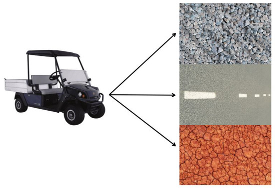
Figure 1.
An example showcasing the three types of terrain on which vehicles can travel is presented. Specifically, the top image displays a gravel terrain, followed by a pavement terrain in the middle, and finally a clay terrain at the bottom.
The estimation of IPC of an EV following a trajectory cannot be accomplished solely with voltage and battery measurement data, but it must also encompass certain terrain characteristics. Several authors have tackled the modeling of IPC in EVs from various perspectives, yielding diverse outcomes [5,11,15,18,19]. These investigations have underscored a pronounced reliance on vehicle dynamics [20]. Satellite information enables the acquisition of data concerning trajectory and terrain characteristics, such as altitude, distances, and terrain type, within a map [21,22,23,24]. Moreover, research has been conducted on the identification of features in satellite images, facilitating automated land classification [25].
To address the challenge of IPC estimation along a predefined trajectory, this study presents a methodology that leverages satellite information to establish a connection between the physical phenomena of EV-terrain interaction. Relevant features are extracted for the model, and IPC is computed across three terrain types: pavement, clay, and gravel. Subsequently, a comparison is drawn between these results and measurements obtained from field tests conducted along the same trajectory.
This work is organized as follows: Section 2 presents the problem statement and the mathematical formulation of IPC. Section 3 describes the methodology developed to estimate IPC using satellite information. Section 4 presents the experimental setup, field results, and concludes with a statistical comparison between the proposed methodology, field tests, and manufacturer-provided information. Finally, Section 5 presents the main conclusions of this work.
2. Problem Statement
The IPC can be directly measured from the vehicle’s batteries by obtaining the product of voltage and current, as shown in Equation (1).
where V and I represent the battery voltage and current, respectively, and the subscript t denotes the dependence on time.
Previous works by Gionesmaki [18] and later Iora [19] have indicated that the IPC can be estimated by considering the balance of forces acting on the wheels of the vehicle (See Figure 2). This balance of forces required for wheel traction is presented in Equation (2). It takes into account factors such as the air resistance on front surface of the vehicle, the resistance from the terrain due to the mechanical effects on the wheels, the slope of the terrain, and the acceleration of the vehicle, among others, as shown in Equation (2).
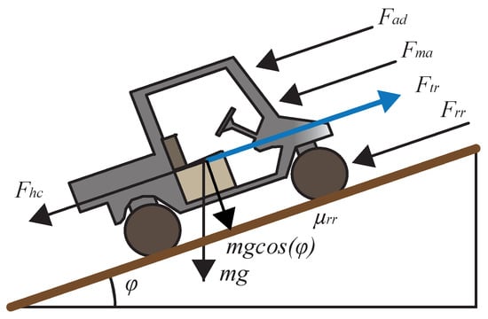
Figure 2.
Forces acting on a vehicle.
Here, represents the traction force, is the aerodynamic force acting on the vehicle due to the air, is the rolling resistance force, and is the acceleration force. These forces can be described as follows:
where is the air density, A is the frontal area of the vehicle, is the drag coefficient, v is the vehicle speed, is the rolling resistance coefficient, m is the vehicle mass (including load), g is the acceleration due to gravity, is the slope of the terrain, and a represents the vehicle acceleration. This equation is valid for steered vehicles with non-deformable wheels [5,11,18].
The power required for wheel traction is a function of the force exerted by the wheels and the speed, as shown below:
The power supplied from the batteries can be determined by , where is the power from the battery, and is the electromechanical conversion efficiency of the vehicle system. It incorporates the efficiency of the battery, the motor, the mechanical transmission from the motor to the wheels, and losses in accessories (e.g., lights, sensors, on-board computer, etc.) other than the motor [18,26]. This efficiency can be obtained from Equation (5).
Here, , , and are the battery, motor, and transmission efficiency, respectively. represents the temperature, and and are the current and resistance of all accessories, respectively. The equation for IPC can then be rewritten as follows:
Based on the above, there are two approaches to acquiring IPC. One method involves directly measuring the battery’s voltage and current. The alternative approach entails estimating the forces implicated in the vehicle’s motion, taking into account the influencing variables. In situations where significant temperature disparities exist, battery performance and lifespan could be impacted [27,28]. Another factor to consider, the focus of this study, is the terrain type, as it exerts an opposing effect on EV movement. Additionally, the terrain may be inclined, which could either facilitate or impede motion depending on the angle of inclination [11,29,30], thus contributing to the IPC calculation.
Having prior knowledge of IPC and a predefined known route allows for effective management, such as determining battery charging points along the trajectory, assessing if the EV can reach its destination with its current autonomy, and optimizing navigation resources, among other benefits [5,31].
Available satellite information enables route planning for navigation from one point to another on a map (e.g., Google Maps, OpenMaps, etc.). Additionally, they provide relevant information to approximate the IPC of an EV. This is the motivation behind using satellite information for IPC estimation in this work.
3. IPC Based in Satellite Information Proposed Methodology
Satellite information provides valuable data for estimating the power consumption of an EV. It includes latitude, longitude, and elevation information on a map, which helps identify the starting and destination points. Indirectly, the distance between two points can be extracted, and with advance knowledge of the speed, the travel time can be determined. Elevation provides an approximation of the terrain slope. Additionally, satellite maps offer visual representations of terrain characteristics, allowing for terrain classification and the association of their respective effects on vehicle movement opposition. Approaches to these effects have been addressed by Romero Schmidt and Auat [11], who proposed data acquisition through visual classification techniques using support vector machines (SVM) and established the relationship between speed and IPC consumption in four types of terrain: clay, grass, gravel, and pavement. Subsequently, Villacrés and Auat [5] conducted experiments that collected IPC data, establishing a polynomial model adjusted through a piecewise regression algorithm, enabling the correlation of velocity and IPC in three different types of terrain. These works, particularly in the experimental results, assume constant mass and velocity and are carried out on flat terrain, disregarding the slope.
Based on the aforementioned, this paper aims to estimate IPC using satellite information while considering the effects of terrain and slope. The methodology is illustrated in Figure 3. In this methodology, the satellite information used is considered to be the position in latitude, longitude and altitude, and the image in which the trajectory is fitted. The estimation of the IPC is made prior to traveling the defined trajectory. Therefore, satellite information on the vehicle speed is not considered.
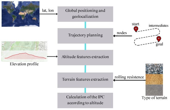
Figure 3.
Schematic of the proposed methodology.
3.1. Global Positioning and Geolocation
The process begins by acquiring satellite information of a given city or location using platforms such as Google Maps and OpenStreetMap. This information provides latitude and longitude data. The latitude and longitude allow for the identification of the vehicle’s location in space, which can then be georeferenced on a map. To achieve this, an image is obtained, and the coordinates of the image’s corners are known.
Georeferencing enables working with the image using the global position information provided by latitude and longitude and transforming it into x and y coordinates with respect to a reference frame.
3.2. Trajectory Planning
The definition of the trajectory is essential to determine how the vehicle will travel from a starting point A to a destination point B. This involves moving along the map following a route that connects A and B, with intermediate points that the vehicle must pass through. This can be represented as a series of nodes, which represent the points, and arcs, which represent the connections between these points.
In this methodology, the starting point, intermediate points, and destination point are arbitrarily determined to create a predefined route. However, different strategies can be considered for route construction. For example, in street navigation, a start and end point can be specified, and the intermediate points can depend on the streets, intersections, etc. This allows the establishment of adjacency between nodes for subsequent optimization.
Considering that navigation encompasses various terrain types and not just road or pavement conditions, only points that allow navigation along the trajectory and are reachable are taken into account.
3.3. Altitude Feature Extraction
The nodes positioned along the trajectory need to have information about their geographical position to be accurately placed on the georeferenced image. Additionally, each node should have elevation information corresponding to its location. This elevation information is not readily available for free from platforms like Google Maps or OpenStreetMap. However, there are APIs available, such as Open-Elevation (open-elevation.com (accessed on 30 October 2023)), that can be used to obtain elevation data. These APIs accept latitude and longitude coordinates as input and provide elevation information as output. Alternatively, manual methods can be employed, as some service providers offer on-screen altitude or elevation information.
It is important to note that the elevation information obtained is based on topographic contour lines, and there may be errors in determining the exact height of a point on the map due to surface irregularities. Nevertheless, these data allow for an approximate estimation of the slopes between nodes.
3.4. Terrain Features Extraction
The georeferenced satellite image provides a visual representation of various types of terrain. Streets appear as gray surfaces, grass or wooded areas as green, and dirt and clay surfaces as brown. Consequently, it is possible to label the arcs between nodes based on the types of terrain that the vehicle may navigate. In this methodology, the labeling of arcs is performed manually. Each node was labeled considering the color of the surrounding terrain, defining each node in three categories: pavement, clay and gravel, according to whether the terrain is light gray, brown, and gray, respectively. However, the utilization of image processing techniques for feature extraction to classify the terrain like proposed in [5,11] in is not disregarded.
3.5. Calculation of the IPC
First, the distance and slope between adjacent points need to be calculated.
The distance between nodes can be determined using the Euclidean distance formula, considering that the position data are known, as shown in Equation (7). This, considering that the difference in height is negligible between nodes.
Here, represents the distance between nodes i and j, and , , , and denote the position coordinates of the respective nodes.
The angle of elevation between nodes is determined using Equation (8), where and represent the elevations at nodes i and j, respectively.
Then, the IPC is calculated for each pair of nodes, considering a predefined speed for traversing the predefined trajectory, the mass of the vehicle (including passengers and cargo), the terrain elevation, the type of terrain, and its corresponding rolling resistance coefficient. Equation (6) is used, where each parameter and variable is substituted accordingly. Since the navigation time between nodes is known, an estimate of the energy consumption for the given route can be obtained. This cumulative effect is applied to each pair of nodes until the entire path between the starting and destination nodes is completed.
4. Experiments
This section presents the results of the computational experiments performed using the proposed methodology, as well as the details of the experimental setup and the validation results. In Table 1 is summarized the experiments and data to use. In the case of direct measurement, it is obtained during field experiment to be used for validation.

Table 1.
Types of experiments and data setup for variables to obtain IPC.
4.1. Computational Experiments
The computational experiments were conducted at the map of the facilities of Universidad Técnica Federico Santa María, located in Viña del Mar, Valparaíso, Chile.
A satellite image of the area was obtained from Google Maps using the Sas Planet 2022 software. The image captures three different terrains to be studied: gravel, clay, and pavement. The latitude and longitude coordinates of the upper left (−33.03856107, −71.48669920) and lower right (−33.04012602, −71.48467145) corners of the image were collected for georeferencing purposes. The image and coordinates were transformed into meters for distance analysis between nodes and into pixels for interaction with the image, as shown in Figure 4 (north points upwards).
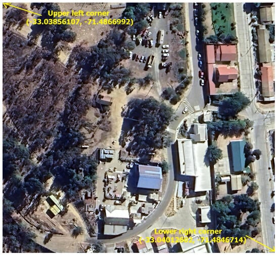
Figure 4.
Selected area of the facilities of Universidad Técnica Federico Santa María, Viña del Mar, Valparaíso, Chile (https://goo.gl/maps/yscek8oYisThQJTT6) accessed on 12 July 2023.
The starting and ending points of each trajectory were determined to create three routes: gravel, clay, and pavement. These routes are depicted in Figure 5, with points A and B representing the start and goal, respectively.
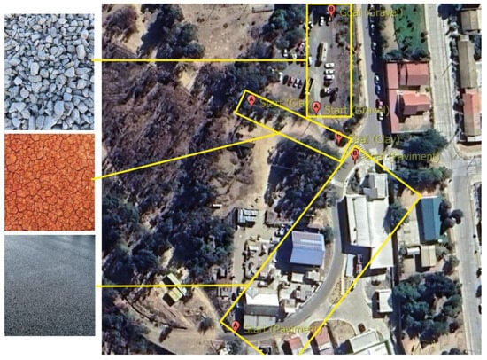
Figure 5.
Designed trajectories in gravel, clay, and pavement (ordered from top to bottom).
A total of 8 nodes were placed along each trajectory, including the start, intermediate, and goal nodes, which were evenly spaced. The longest trajectory covered a distance of 105 m. Once the nodes were determined, their elevations were obtained using the open-elevation API based on their latitude and longitude coordinates (see Figure 6).
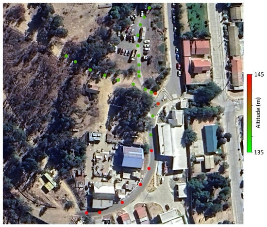
Figure 6.
Nodes of trajectories in gravel, clay, and pavement colored according to altitude. Red represents the maximum altitude, and green represents the minimum altitude.
With the nodes and their information available, the next step was to calculate the distance and slope between them. To calculate the IPC, certain parameters or variables needed to be established in advance. The speed was set at 5, 4 and 3 m/s for pavement, clay, and gravel, respectively, as it is essential for determining the time between each section of the trajectory. Given the speed, the effect of air resistance on the vehicle can be assumed to be negligible due to its quadratic dependence. The IPC calculation demonstrated varying behavior with slope and terrain type along the trajectory.
4.2. Experimental Setup
The Cushman Hauler Pro electric vehicle was used for the experimental study. This vehicle is equipped with an AC motor and has a seating capacity for two people. An RTK (Real-Time Kinematics) system was installed on the roof of the vehicle to obtain accurate position data along the route.
Table 2 provides the characteristics of the hardware used in the setup, including the electric vehicle specifications, the RTK GNSS (Navcom SF-3040) details, the IMU (Vectornav VN-200) specifications, and the voltage and current sensor specifications.
Table 2.
Characteristics of the Hardware Setup.
The vehicle’s speed is estimated based on the predefined route and the time sampling. An IMU (Inertial Measurement Unit) Vectornav VN-200 is installed to gather information about the vehicle’s inclination and, consequently, the slopes encountered during the trials. Additionally, a voltage and current sensor is connected to the batteries to calculate the IPC.
The IPC sensor used in the study is depicted in the schematic shown in Figure 7. The sensor consists of voltage and current inputs that allow for the measurement of IPC.
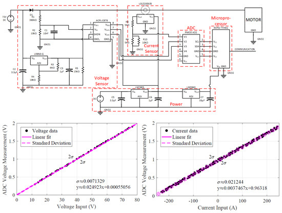
Figure 7.
Circuit schematic and curve of operation for the voltage and current inputs of the IPC sensor.
The inputs of voltage and current are designed to operate within specific ranges. The curve in Figure 7 illustrates the relationship between the input voltage and current. It demonstrates how the sensor adapts and converts the battery voltage and current signals into measurable values.
The voltage input range of the sensor extends from 0 to 80 V. This range is adjusted using voltage dividers to ensure accurate measurements within the 0–2 V output range. Similarly, the current input range is accommodated by the sensor, allowing for measurements within the 0–2 V range. The analog signals from both inputs are then converted to digital signals and read by a microcontroller for further processing.
Overall, the IPC sensor and its operational characteristics enable the accurate measurement and monitoring of voltage and current, facilitating the estimation of IPC in the study.
All this information, from RTK, IMU, and IPC sensors, is acquired and processed by the industrial on-board computer, using the Ubuntu operating system with ROS implemented. The specifications of the hardware used are detailed in Table 2 and the experimental setup is shown in Figure 8, where the platform used and the sensors mounted are shown.
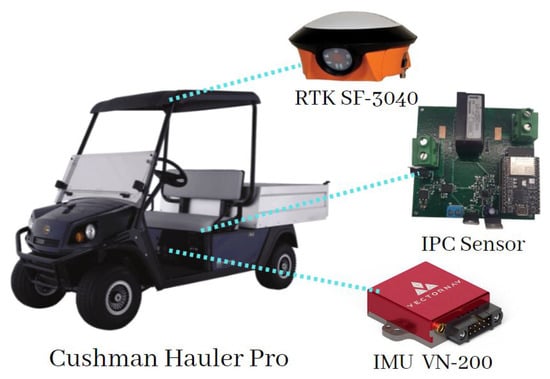
Figure 8.
Electric vehicle used for field testing, equipped with an RTK system, an IMU, and an IPC (voltage and current) sensor connected to the batteries.
4.3. Field Experiments
Field tests were conducted at the facilities of the Universidad Técnica Federico Santa María in Viña del Mar, Valparaíso, Chile. Three routes were established, each with a different type of terrain: pavement, clay, and gravel, based on the simulation trajectories.
The following experiments were conducted:
- 10 trials in pavement terrain.
- 10 trials in clay terrain.
- 10 trials in gravel terrain.
In each of these trials, measurements from RTK, IMU, and IPC sensors were collected along their trajectories.
The main objective of these measurements was to collect data to visualize the effects of the elevation angle on the IPC and to gather information on the global position of the vehicle for trajectory reconstruction. The data were processed considering the velocity and acceleration behavior, and a reference IPC was generated by directly measuring the data from the batteries.
Figure 9 shows the nodes where RTK measurements were taken, along with their corresponding altitudes. The vehicle traveled from the lowest altitude zone to the highest altitude zone, encountering a positive elevation angle for most of the journey.
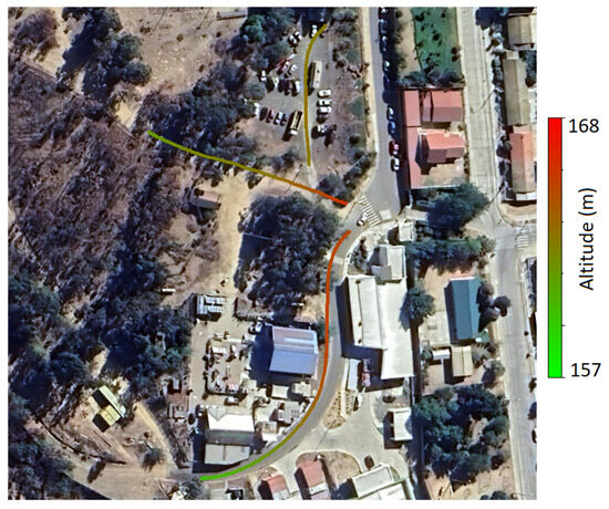
Figure 9.
Nodes and altitudes measured in each trajectory.
5. Results
Figure 10 shows the data obtained from the RTK, IMU, and IPC sensor measurements on the three types of terrain. The height, velocity, acceleration, and IPC data are presented with respect to the number of measurements synchronized by the slowest sensor, in this case, the RTK, which has a sampling time of 0.3 s.
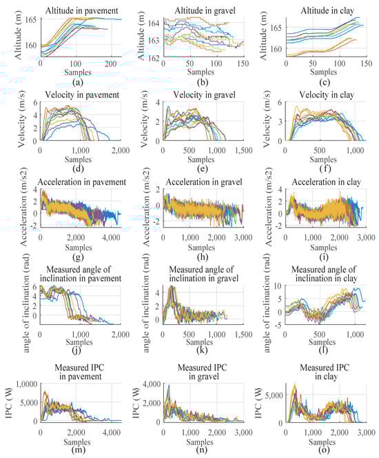
Figure 10.
Raw data. In (a–c), altitude samples during the vehicle’s travel are shown across pavement, gravel, and clay, respectively. Letters (d–f) depict the vehicle speed measured through the IMU for the three types of terrains. In (g–i), acceleration samples for the three terrains are displayed. In (j–l), the inclination angle of each terrain is shown based on the pitch obtained from the IMU. Using the IPC sensor, curves (m–o) were obtained to visualize the behavior of battery power consumption during each trial.
In Figure 10a, it is evident that the trajectory on pavement reveals fluctuations in the vehicle’s altitude relative to sea level as it progresses at the onset of the journey. In gravel, illustrated in Figure 10b, a consistent behavior is observed, demonstrating variations in routes and even between trials, notwithstanding the ostensibly flat terrain. Conversely, the altitude in clay, as illustrated in Figure 10c, displays a pattern akin to that of the pavement–initiating at a lower altitude and gradually ascending. However, two of the trials exhibit deviations in height measurements. It is crucial to note that along this trajectory, there exists abundant vegetation and trees that could potentially impact RTK data acquisition. Nonetheless, the trajectory follows a pattern similar to the other trials. It is essential to emphasize that, for the subsequent utilization of altitude data, only its variation is relevant for estimating the terrain’s incline angle.
Graph Figure 10d illustrates the speed profiles developed in the 10 trials conducted on paved terrain. The profile is not uniform across each trial, given that the vehicle was manually driven without speed control. Nevertheless, a resemblance is noted among most trials, with speeds consistently hovering around 5 m/s. Additionally, the effects of acceleration and braking are discernible at the beginning and end of the run, respectively.
In the case of the gravel speed (see Figure 10e, there is an observable variation in speed within the intermediate samples of the trajectory. Concerning the phenomena witnessed on the ground, instances of the vehicle sliding and skidding were noted at specific points along the route.
As for the speed on clay, depicted in Figure 10f, a stable speed behavior is evident, with trials exhibiting very similar patterns across various samples and reaching a development speed of 4 m/s.
Regarding the acceleration derived from the IMU, graphs Figure 10g–i depict the acceleration on pavement, gravel, and clay, revealing a noticeable noisy behavior that consistently hovers around 0 for most of the route. The exception to this is evident at the edges of the graphs, where the effects of startup are observed as the vehicle transitions from inertia, and at the end, during the braking action.
When measuring the vehicle’s lean angle with the IMU using pitch data, given its close alignment with the vehicle’s straight line, these angles are illustrated in Figure 10j for pavement, Figure 10k for gravel, and Figure 10l for clay. Moreover, it is observable that the inclination behaviors align with the variations in the previously mentioned altitudes. In the case of pavement, a pronounced inclination angle is noted at the beginning, gradually reducing until it reaches a relatively flat position with an inclination close to 0. On gravel, constant jumps in the measurements are apparent. Meanwhile, on clay, the inclinations display two slopes with an intermediate flat sector. In Figure 10m–o, the IPC measurements directly measured from the EV battery are presented for the experiments on pavement, gravel, and clay. The behavior of these measurements shows a strong relationship with the slope of the terrain since they follow a similar graphical shape.
With the data collected in the experiments, the measurements were compared with the estimates from the field experiments. Figure 11 shows plots of IPC over time and IPC versus velocity obtained in the three types of terrain analyzed. These graphs are generated by estimating the IPC through Equation (9) and plotting the results against their corresponding velocities.
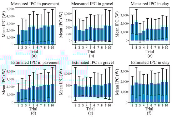
Figure 11.
IPC in field experiments and IPC measures. Figures (a–c) depict the average IPC measurements and standard deviation from the 10 field trials on pavement, gravel, and clay, respectively. In (d–f), the average IPC estimates are presented using data from the sensors utilized in the field trials.
In Figure 12a, the estimated IPC with the sensor data for the pavement is presented. Inputting the sensor inputs and parameters (mass, gravity, rolling coefficient) into the model produces a curve describing power consumption that closely resembles the one measured from the battery, as shown in Figure 12d. In Figure 12b, there is a notable variation in the IPC for the gravel trajectory due to the variable and noisy nature of the collected data, exhibiting partial similarity with the IPC measured in Figure 12e. A distinct section reveals an increase in the magnitude of the IPC. However, the influence of the angle of inclination displays a negative behavior, potentially associated with a regenerative braking phenomenon. This behavior is attributed to the constant variation of the inclination and intermittent contact with the terrain. Similarly, in Figure 12c, a comparable behavior is observed between the model’s estimated IPC and its battery-measured counterpart. In Figure 12g–i, the ratios of the IPC estimated in the terrain tests to the measured speed for each type of terrain are depicted. Meanwhile, Figure 12j–l illustrate the ratio of the measured IPC to speed. In the ratios of estimated IPC to speed, the presence of both positive and negative power consumption occurrences at different speeds is diluted, aligning with expected effects of the model tilt angle.
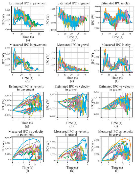
Figure 12.
IPC graphics. (a–c) display the IPC estimates for pavement, gravel, and clay over time. Similarly, in (d–f), the IPC measurements for the same soils are shown. In (g–i), the estimated IPC behavior curves concerning speed are presented. In the case of (j–l), we can observe the behavior of the measured IPC with respect to speed. In these graphs, both positive and negative IPC can be observed, mainly associated with acceleration and braking, as well as the effects of slope and the type of terrain.
The information regarding the IPC from the estimations and measurements conducted in the field is presented in Figure 11.
This figure summarizes the averages and standard deviations of each of the trials carried out in the experiments on the three types of terrain. The estimated IPC averages presented in Figure 11a–c exhibit significant similarity to the battery measurements for all three experimented terrains. However, it is observed that there is a substantial standard deviation in each experiment, which, in turn, is consistent with its measurement.
The results of the computational experiment, field experiments, and direct battery measurements of the EV to obtain the average IPC on the three types of analyzed terrain are shown in Figure 13. It can be observed that the performance of the computational experiment, which utilizes information from a georeferenced image and its height data, presents an error of 5.43% for clay, 19.19% for pavement, and 102.20% for gravel. The latter exhibits poor performance, considering that satellite images lose the quality of the real terrain, coupled with phenomena arising from gravel terrain, such as skidding, wheel burying, or even favorable effects allowing the vehicle to slide on slight slopes. Additionally, differences in height acquisition of around 15 m were observed with an error of 3 m. On the other hand, estimates based on the on-site experiment using RTK and IMU present an error of 5.11% for gravel, 14.50% for pavement, and 21.25% for clay. This performance is quite close to the directly measured battery values, which, when fed into the model with greater precision and accuracy, would allow for an estimation through the EV’s longitudinal dynamics very close to reality.
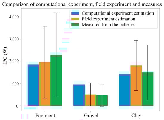
Figure 13.
The graph provides a visual representation of the IPC values for different terrains: pavement, gravel, and clay. It shows that the estimation using satellite information, the experimental estimation, and direct measurements from the batteries.
6. Conclusions
The presented study has introduced a novel methodology for IPC estimation leveraging satellite information, employing nodes defined by latitude, longitude, elevation, and terrain type data. The application of this method across three distinct terrains—gravel, clay, and pavement—revealed promising results. Notably, the simulation demonstrated a satisfactory approximation for pavement and clay terrains. Nevertheless, the estimation performance for gravel terrain demands further scrutiny, particularly concerning the accuracy of the measured IPC.
Field experiments were conducted to collect data on position over time and elevation angles along the trajectory for IPC estimation. Moreover, direct measurements of IPC were obtained from the batteries, serving as a benchmark for comparison.
Despite the challenges encountered, particularly in the case of gravel terrain, this research significantly contributes to the field of IPC estimation for electric vehicles. The utilization of satellite data and field experiments showcases the potential of the proposed methodology. The observed discrepancies in gravel terrain underscore the complexities associated with dynamic terrains, emphasizing the need for refinement and adaptation of the methodology to address specific challenges presented by such conditions.
Looking ahead, potential future work should focus on optimizing the IPC estimation model, with a particular emphasis on refining the algorithm for gravel terrain. Incorporating additional factors, such as real-time environmental conditions, filtered data, and improved sensor technologies, could further enhance the accuracy and applicability of the proposed method. Additionally, exploring the integration of machine learning techniques to adapt and learn from real-world experiences may contribute to overcoming challenges and improving overall performance. This study lays the foundation for future research in the realm of IPC estimation, offering valuable insights and paving the way for advancements in electric vehicle technology.
Author Contributions
Conceptualization, F.J. and F.A.; methodology, F.J. and F.A.; software, F.J.; validation, F.J. and J.E.; formal analysis, F.J. and J.E.; investigation, F.J.; resources, F.A.; data curation, F.J. and J.E.; writing—original draft preparation, F.J. and J.E.; writing—review and editing, F.J., J.E. and F.A.; visualization, F.J. and J.E.; supervision, F.A.; project administration, F.A.; funding acquisition, F.A. All authors have read and agreed to the published version of the manuscript.
Funding
This work was partially supported by the Advanced Center for Electrical and Electronic Engineering, AC3E, ANID basal project FB0008.
Data Availability Statement
Not applicable.
Conflicts of Interest
The authors declare no conflict of interest.
References
- Ding, X.; Guo, H.; Xiong, R.; Chen, F.; Zhang, D.; Gerada, C. A new strategy of efficiency enhancement for traction systems in electric vehicles. Appl. Energy 2017, 205, 880–891. [Google Scholar] [CrossRef]
- Albatayneh, A.; Assaf, M.; Alterman, D.; Jaradat, M. Comparison of the Overall Energy Efficiency for Internal Combustion Engine Vehicles and Electric Vehicles. Rigas Teh. Univ. Zinat. Raksti 2020, 24, 669–680. [Google Scholar] [CrossRef]
- Jiang, X.; Chen, L.; Xu, X.; Cai, Y.; Li, Y.; Wang, W. Analysis and optimization of energy efficiency for an electric vehicle with four independent drive in-wheel motors. Adv. Mech. Eng. 2018, 10, 1687814018765549. [Google Scholar] [CrossRef]
- Mansour, C.; Haddad, M.; Zgheib, E. Assessing consumption, emissions and costs of electrified vehicles under real driving conditions in a developing country with an inadequate road transport system. Transp. Res. Part D Transp. Environ. 2018, 63, 498–513. [Google Scholar] [CrossRef]
- Villacrés, J.; Cheein, F.A. In-field piecewise regression based prognosis of the IPC in electrically powered agricultural machinery. Comput. Electron. Agric. 2022, 202, 107324. [Google Scholar]
- Naik, S.; Mallur, S. Performance analysis and energy saving opportunities for agricultural implements and tractor trailer industries. Int. J. Sci. Technol. Res. 2019, 8, 1772–1776. [Google Scholar]
- Guevara, L.; Michałek, M.; Auat Cheein, F. Headland turning algorithmization for autonomous N-trailer vehicles in agricultural scenarios. Comput. Electron. Agric. 2020, 175, 105541. [Google Scholar] [CrossRef]
- Guevara, L.; Rocha, R.; Cheein, F. Improving the manual harvesting operation efficiency by coordinating a fleet of N-trailer vehicles. Comput. Electron. Agric. 2021, 185, 106103. [Google Scholar] [CrossRef]
- Prasad, R.; Shankar, P.S. Efficient performance analysis of energy aware on demand routing protocol in mobile ad-hoc network. In Engineering Reports; John Wiley & Sons Ltd.: Hoboken, NJ, USA, 2020; Volume 2, p. e12116. [Google Scholar]
- Zhang, S.; Gajpal, Y.; Appadoo, S.; Abdulkader, M. Electric vehicle routing problem with recharging stations for minimizing energy consumption. Int. J. Prod. Econ. 2018, 203, 404–413. [Google Scholar] [CrossRef]
- Romero Schmidt, J.; Auat Cheein, F. Prognosis of the energy and instantaneous power consumption in electric vehicles enhanced by visual terrain classification. Comput. Electr. Eng. 2019, 78, 120–131. [Google Scholar] [CrossRef]
- Xu, X.; Aziz, H.A.; Guensler, R. A modal-based approach for estimating electric vehicle energy consumption in transportation networks. Transp. Res. Part D Transp. Environ. 2019, 75, 249–264. [Google Scholar] [CrossRef]
- Weiss, M.; Cloos, K.C.; Helmers, E. Energy efficiency trade-offs in small to large electric vehicles. Environ. Sci. Eur. 2020, 32, 1–17. [Google Scholar]
- Cheon, S.; Kang, S.J. An electric power consumption analysis system for the installation of electric vehicle charging stations. Energies 2017, 10, 1534. [Google Scholar] [CrossRef]
- Bustos, J.T.; Orchard, M.E.; Torres-Torriti, M.; Cheein, F.A. GNSS-Based Estimation of Average Instantaneous Power Consumption in Electric Vehicles. IEEE Trans. Ind. Electron. 2022, 70, 9281–9290. [Google Scholar] [CrossRef]
- Semeraro, F.F.; Schito, P. Numerical Investigation of the Influence of Tire Deformation and Vehicle Ride Height on the Aerodynamics of Passenger Cars. Fluids 2022, 7, 47. [Google Scholar] [CrossRef]
- Kremzow-Tennie, S.; Hellwig, M.; Pautzke, F. A study on the influencing factors regarding energy consumption of electric vehicles. In Proceedings of the 2020 21st International Conference on Research and Education in Mechatronics (REM), Cracow, Poland, 9–11 December 2020; pp. 1–6. [Google Scholar]
- Genikomsakis, K.; Mitrentsis, G. A computationally efficient simulation model for estimating energy consumption of electric vehicles in the context of route planning applications. Transp. Res. Part D Transp. Environ. 2017, 50, 98–118. [Google Scholar] [CrossRef]
- Iora, P.; Tribioli, L. Effect of ambient temperature on electric vehicles energy consumption and range: Model definition and sensitivity analysis based on nissan leaf data. World Electr. Veh. J. 2019, 10, 2. [Google Scholar] [CrossRef]
- Tran, D.D.; Vafaeipour, M.; El Baghdadi, M.; Barrero, R.; Van Mierlo, J.; Hegazy, O. Thorough state-of-the-art analysis of electric and hybrid vehicle powertrains: Topologies and integrated energy management strategies. Renew. Sustain. Energy Rev. 2020, 119, 109596. [Google Scholar]
- Li, X.; Qin, Z.; Shen, Z.; Li, X.; Zhou, Y.; Song, B. A High-Precision Vehicle Navigation System Based on Tightly Coupled PPP-RTK/INS/Odometer Integration. IEEE Trans. Intell. Transp. Syst. 2023, 24, 1855–1866. [Google Scholar] [CrossRef]
- Yamasaki, Y.; Noguchi, N. Research on autonomous driving technology for a robot vehicle in mountainous farmland using the Quasi-Zenith Satellite System. Smart Agric. Technol. 2023, 3, 100141. [Google Scholar] [CrossRef]
- Wu, M.; He, Y.; Wu, H.; Liu, W. Multi-dimensional particle filter-based estimation of phase line biases for single-differenced ambiguity resolution in GNSS-based attitude determination. Meas. Sci. Technol. 2023, 34, 025026. [Google Scholar] [CrossRef]
- Masood, K.; Zoppi, M.; Molfino, R. Mathematical Modelling for Performance Evaluation Using Velocity Control for Semi-autonomous Vehicle. In Proceedings of the International Workshop on Soft Computing Models in Industrial and Environmental Applications, Burgos, Spain, 16–18 September 2020; Springer: Berlin/Heidelberg, Germany, 2020; pp. 617–626. [Google Scholar]
- Saha, S.K. Remote Sensing and Geographic Information System Applications in Hydrocarbon Exploration: A Review. J. Indian Soc. Remote Sens. 2022, 50, 1457–1475. [Google Scholar] [CrossRef]
- Zhou, S.; Wang, Q.; Liu, J. Control Strategy and Simulation of the Regenerative Braking of an Electric Vehicle Based on an Electromechanical Brake. Trans. FAMENA 2022, 46, 23–40. [Google Scholar] [CrossRef]
- Ma, S.; Jiang, M.; Tao, P.; Song, C.; Wu, J.; Wang, J.; Deng, T.; Shang, W. Temperature effect and thermal impact in lithium-ion batteries: A review. Prog. Nat. Sci. Mater. Int. 2018, 28, 653–666. [Google Scholar] [CrossRef]
- Wu, W.; Wang, S.; Wu, W.; Chen, K.; Hong, S.; Lai, Y. A critical review of battery thermal performance and liquid based battery thermal management. Energy Convers. Manag. 2019, 182, 262–281. [Google Scholar] [CrossRef]
- Reina, G.; Galati, R.; Milella, A. All-terrain estimation for mobile robots in precision agriculture. In Proceedings of the 2018 IEEE International Conference on Industrial Technology (ICIT), Lyon, France, 19–22 February 2018; pp. 63–68. [Google Scholar]
- Taghavifar, H.; Rakheja, S. A novel terramechanics-based path-tracking control of terrain-based wheeled robot vehicle with matched-mismatched uncertainties. IEEE Trans. Veh. Technol. 2019, 69, 67–77. [Google Scholar] [CrossRef]
- Ghobadpour, A.; Monsalve, G.; Cardenas, A.; Mousazadeh, H. Off-Road Electric Vehicles and Autonomous Robots in Agricultural Sector: Trends, Challenges, and Opportunities. Vehicles 2022, 4, 843–864. [Google Scholar] [CrossRef]
Disclaimer/Publisher’s Note: The statements, opinions and data contained in all publications are solely those of the individual author(s) and contributor(s) and not of MDPI and/or the editor(s). MDPI and/or the editor(s) disclaim responsibility for any injury to people or property resulting from any ideas, methods, instructions or products referred to in the content. |
© 2023 by the authors. Licensee MDPI, Basel, Switzerland. This article is an open access article distributed under the terms and conditions of the Creative Commons Attribution (CC BY) license (https://creativecommons.org/licenses/by/4.0/).