Abstract
Learning-based control systems have shown impressive empirical performance on challenging problems in all aspects of robot control and, in particular, in walking robots such as bipeds and quadrupeds. Unfortunately, these methods have a major critical drawback: a reduced lack of guarantees for safety and stability. In recent years, new techniques have emerged to obtain these guarantees thanks to data-driven methods that allow learning certificates together with control strategies. These techniques allow the user to verify the safety of a trained controller while providing supervision during training so that safety and stability requirements can directly influence the training process. This survey presents a comprehensive and up-to-date study of the evolving field of stability certification of neural controllers taking into account such certificates as Lyapunov functions and barrier functions. Although specific attention is paid to legged robots, several promising strategies for learning certificates, not yet applied to walking machines, are also reviewed.
1. Introduction
Stability is a fundamental requirement from an engineering perspective since it guarantees that the controlled system, under bounded disturbances, can wander in a limited region of state space. While stability theory had a huge impact on the design of controllers for linear systems, it is quite difficult to provide stability guarantees in the nonlinear case. Since the beginning of 2000, barrier and Lyapunov certificates have been provided as a practical method for formally proving the stability and safety of nonlinear and hybrid systems [1,2]. However, it was possible to find these functions using traditional methods, with much time and effort invested in customising unique certificates for specific systems. The problem becomes even more difficult for multi-body mechanical structures, such as legged machines, where assimilation to linear dynamics is often at the expense of the reliability of the defined controller. The search for stability guarantees for this class of complex mechanical systems becomes an urgent challenge as legged robots are becoming increasingly popular [3,4]. They are expected to complement traditional wheeled machines due to their dexterity and ability to explore highly unstructured terrains with minimal invasiveness. Consider, for example, the inspection of landslide [5,6] areas for monitoring and sensor deployment: here, you have to move through slippery and steep terrains that are often inaccessible to robots on wheels or from the air for the presence of vegetation. These terrains are the natural habitat of animals, especially insects and quadrupeds, showing that the most reliable solution for natural terrain exploration is the use of legged robots [7].
Legged robots are a type of mobile robot that uses articulated limbs such as leg mechanisms for locomotion. Thanks to their ability to change the configuration of their legs and adapt to the surface, they can move remarkably well over natural terrain. However, achieving the dynamic stability of a legged robot when walking or running is a major challenge. It is crucial to determine the position of its feet and avoid falls when reaching its destination. This challenge arises from the fact that locomotion requires contact forces with the environment, which are constrained by the mechanical laws of contact and the limits of robot actuation [8].
Complex control routines require precise modelling phases. Due to the high complexity of legged robot bodies and the peculiarities of their specific structures, standardised models and associated model-based techniques are often of limited suitability for direct application for control purposes. On the other hand, the use of sophisticated simulation environments and the use of data recorded directly from the robot’s onboard devices makes the use of data-driven strategies significantly relevant.
More recently, data-driven learning methods have expanded beyond such traditional areas as image processing and general classification or regression modelling to areas closely related to stability and safety state evaluation. While neural-network-based methods have been used for many years for high-level navigation [9,10], there have been difficulties in closing the loop for low-level motion control due to a lack of stability guarantees. Only recently the first results on the fulfilment of stability and safety guarantees in the synthesis of controllers for dynamical systems have been investigated, especially in safety-critical applications such as autonomous vehicle systems [11] and simple models of robotic systems such as the inverted pendulum [12,13]. From then on, increasing amounts of cases have been studied, accompanied by several slightly different approaches to formally synthesise stable and safe controllers through learning techniques. While most of them refer to wheeled robots, there are at the same time many cases reporting the application of data-driven methods to legged robots for solving the stability and safety problem. In addition, other methods that may be of interest in this area have not yet been applied to legged robots.
Due to the relatively recent interest in the problem of learning stability certificates, there are few review papers in this area [14,15,16,17] and to the best of the authors’ knowledge, none of them were specifically focused on legged robots. On the other hand, there are other approaches to achieve and improve the robustness of legged robots that, although based on learning strategies, do not focus on Lyapunov or Barrier function distillation. Among these, the zero moment point (ZMP) has been considered as a stability indicator that can be learned in legged machines. In [18], and later in [19], a bipedal robot was considered in which an online control strategy based on Iterative Learning Control (ILC) was implemented to improve control performance during a predominantly repetitive task such as walking by using previously memorised control sequences. Other approaches utilise reinforcement learning. Based on the above considerations, this paper discusses the current state of the art in the design of stability and barrier functions as well as the corresponding certificate functions such as Control Lyapunov Functions (CLFs) and Control Barrier Functions (CBFs), as illustrated in Figure 1. Other approaches to data-driven techniques that exploit the potential of reinforcement learning and hybrid solutions are also discussed. We are focusing in particular on learning systems based on neural networks and are deepening our special interest in applications for walking robots.
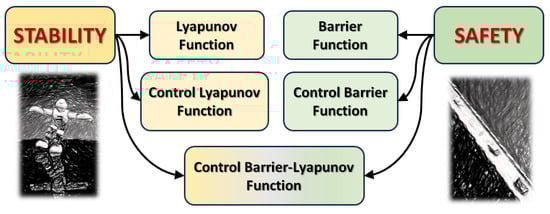
Figure 1.
Description of the different stability and safety certificates taken into consideration.
The role of data-driven techniques such as artificial neural networks (ANNs) in developing appropriate models and certificate functions for legged applications is one of the key elements to emphasise. When controlling dynamical systems, the availability of an accurate model is essential, but this requirement is not always satisfied. On the other hand, nowadays, huge amounts of data are usually available and the possibility of obtaining realistic measurements of the process to be controlled is not prohibitive thanks to inexpensive storage devices. The problem that needs to be solved is how to properly use these data or measurements to extract knowledge or derive a model from the measurements through learning. This approach becomes unavoidable when the mathematical description of the system dynamics becomes too complex or when the gap between the approximated and the real system grows due to the dominance of those dynamics that cannot be modelled analytically. ANNs are among the structures best suited to create input–output mappings from data, which recalls the mathematical problem of approximating generic functions. In 1989, Cybenko formally demonstrated the enormous potential of these structures by emphasising that a neural network with only one hidden layer can always approximate a continuous function with multiple variables with an arbitrary degree of accuracy [20]. Since then, ANNs have proven to be valuable computational paradigms in a variety of applications. Unlike other mathematical models, ANNs offer unique advantages over more classical techniques in areas such as pattern recognition, classification, and system modelling, as they can extract the exemplar starting from the relevant instances provided by examples through learning. Although two main training methods have traditionally been applied to ANNs (i.e., supervised and unsupervised learning), reinforcement learning (RL) has recently gained considerable attention in industry and academia due to its effectiveness in solving complicated problems that require directly deploying the agent in a dynamic environment and learning a strategy optimised by interacting with the environment. Typical applications can be found in the field of autonomous driving, task planning and other areas [21,22]. Learning with the addition of certificates for stability and safety provides a reliable method to control and improve learning by finding more reliable and robust solutions.
Another important topic is the hardware implementation of complex controllers, which often have difficulties in meeting real-time specifications. This assumes more relevance when onboard hardware resources in robotics are usually limited, mainly for energy reasons. The issue here is the ability to run a controller at times that are compatible with the control frequency requirements. For example, most of the routines in use today consider model predictive control (MPC), which, since it requires solving an optimization problem online, is hardly compatible with frequency requirements. From this point of view, neural controllers shift the computational load to the offline phase (training) while achieving remarkable time performance in the running phase. The joint ability to learn a controller, including stability and safety conditions, thus represents a valuable tool for the development of real-time strategies that will promote the proliferation of novel and much more sophisticated controllers than nowadays in the near future.
The rest of the paper is structured as follows: Section 2 provides background on dynamical systems, safety theories and learning mechanisms; Section 3 proposes the learning methodologies used for certificate synthesis; Section 4 presents the applications related to legged robots; Section 5 illustrates the future perspectives; and finally, Section 6 draws the conclusions.
2. Background
This section provides a theoretical overview of the main elements used in the methodological part. We begin with the definition of the systems considered with the proper notation and terminology and then examine basic stability theory and safety concepts.
2.1. Classes of Dynamical Systems
In this section, we go through all the different categories of dynamical systems that will be taken into account. For notation, the state vector is defined as , in which X is the set of state variables, whereas the set of initial conditions is defined as .
Definition 1.
A generic autonomous nonlinear time-invariant system can be expressed in the form:
where is the state and f is a nonlinear function. In this case, there is no dependence on inputs.
Definition 2.
A generic non-autonomous nonlinear time-invariant system can be expressed in the form:
where is the state and is the input.
Definition 3.
A control affine system is a system in which the control appears linearly. It can be expressed in the form:
where and , and are generic nonlinear functions.
Definition 4.
A hybrid system is a dynamical system that exhibits both continuous and discrete dynamic behaviour.
Definition 5.
A controlled hybrid system is defined as:
where denotes the vector state, denotes the control input, denotes the system configuration, i = 1, …, I denotes the system mode, is the flow set where the state follows the continuous flow map , where is defined as , and is the jump set states flows discrete jump map , where defined as . In autonomous hybrid systems .
For RL applications, systems are usually modelled with the Markovian decision process (MDP).
Definition 6.
A Markovian decision process is a tuple S, A, T, R in which S is a finite set of states, A a finite set of actions, T a transition function defined as and R a reward function defined as . Given a time t, the transition function depends only on and not on the previous history.
The transition function T and the reward function R together define the model of the MDP.
2.2. Stability Theory: Lyapunov Functions
In dynamical systems, stability refers to the quality of the system’s behaviour over time and, in particular, to the system’s ability to respond to disturbances. We will consider the problem of the stability of equilibrium points, even though the stability of periodic trajectories also plays a crucial role in robot dynamics. For stability in ordinary differential equations, Lyapunov functions generalise the concept of energy associated with a given system. If it is intuitively possible to assign a generalised energy function to a system whose derivative along the system trajectory is non-positive in a particular neighbourhood of the equilibrium point, this means that the system is either conservative or dissipative in this neighbouring locus, implying the simple or asymptotic stability of the equilibrium point. More formally, given an autonomous dynamical system as described in Equation (1):
Definition 7.
Simple stability: The equilibrium point is stable in the sense of Lyapunov at if for any there exists for which it holds:
Definition 8.
Asymptotic stability: An equilibrium point is asymptotically stable at if is stable and locally attractive, i.e.,
Definition 9.
Exponential stability: An equilibrium point is exponentially stable if
where α is called the rate of convergence.
Whether or not a system meets these definitions can be analysed using one of the most commonly used types of certificate: the Lyapunov function.
Definition 10.
Given the system in Equation (1) and considering as an equilibrium point for the system, a continuously differentiable function is a Lyapunov function (LF) if there exists a neighbour of where:
where is the Lie derivative of V along the dynamics f (often denoted .
If a function satisfying these conditions can be found, then the stability of the equilibrium point can be certified via the following theorems.
Theorem 1
(see [23], Theorem 4.1). If V is a Lyapunov function, , with , then the system has a stable equilibrium at with Ω forming the region of attraction (RoA). Moreover, if for all , then the system has an asymptotically stable equilibrium at .
One of the main advantages of the Lyapunov method is to assess the stability of an equilibrium point without explicitly solving the system dynamics. The primary insights are sublevel sets of V (see Definition 11) which exhibit forward invariance, meaning that once the system enters a sublevel set of V, it will remain in that set for all future times, proving stability. Furthermore, if V decreases monotonically and is bounded below, it will eventually approach its minimum value at 0. Intuitively, V can be interpreted as a generalized energy; if the system is strictly dissipative, then it will eventually come to a stop.
A CLF is used to assess whether a controlled system is asymptotically stabilizable, i.e., whether there exists a control action for each state x such that the system can be asymptotically brought to the zero state by applying this control action u. Formally:
Definition 11.
A function :
where is a bounded c-sublevel set of V(x), , is a (local) Control Lyapunov Function for the system in Equation (2) and is the region of attraction for the equilibrium point . Every is asymptotically stabilizable in , i.e.,
The is evaluated along the dynamic:
Considering the exponential stability definition previously given, it is possible to insert constraints relative to the velocity of convergence. Formally, we can change Equation (8) such that:
This new formulation represents the Exponential Control Lyapunov Function, in which is called the decay rate. Therefore, the problem of stabilization of a nonlinear system is reformulated by looking for suitable inputs that stabilise the 1D dynamical system as shown in Equation (10).
2.3. Safety Theory: Barrier Functions and Nagumo’s Theorem
Barrier functions have been introduced to prove the safety of dynamical systems, rather than their stability. In this case, attention is focused no longer on guaranteeing that the trajectories reach the equilibrium point, but rather on ensuring that the state flow will stay confined within a region of interest, considered as a safe region. Safety can be achieved by proving the forward invariance of a given set. The study of safety in dynamical systems was first introduced in the 1940s by Nagumo, who established the necessary and sufficient conditions for the invariance of a set [24]. A way to prove the safety of a system based on Nagumo’s theorem is the barrier function approach, which is elegantly formalised in [25]. A barrier function certifies the existence of a safe subset in which the state can be proven to remain. Formally:
Definition 12.
Definition 13.
A barrier function is a differentiable function that splits the state space X into where and where such that . Overall, has to be such that:
Given this definition, a barrier function can be used to define the safety of the system.
Definition 14.
Given the dynamical system in Equation (1) with the set X, , and , defined as above, if the barrier function is such that:
Then the system in Equation (1) is safe. It is worth noting that condition (13) imposes that whenever x belongs to the boundary between and (i.e., ), the system dynamics is pushed back into .
Definition 15.
Given that the dynamical system in Equation (2) and a function is continuously differentiable and given its zero-super level set , satisfying , if a positive coefficient γ exists such that :
then B(x) is an Control Barrier Function (CBF). Any Lipschitz-continuous control law that satisfies the aforementioned constraint will make the set safe:
for and
More details about CBF can be found in [26].
2.4. Stability and Safety for Controlled Systems: Control Barrier and Control Lyapunov Functions
The integration between the data-driven approach for the synthesis of controllers, the Lyapunov theory for stability definition and, more recently, the barrier function for safety assessment led to a new line of research that opened the way to new methods and applications. As mentioned above, stability and safety certificates are usually achieved through control Lyapunov or Control Barrier Functions. In some cases, a single function called the Control Lyapunov Barrier Function (CLBF) has been introduced as a single certificate that provides both stability and safety. CLBF can be viewed as a CLF where the safe and unsafe sets are contained in sub- and super-level sets, respectively, [27]. Any control law that satisfies Equation (10) makes the controlled system both stable and safe. This reference also describes an extension to robust CLBF in the case of bounded parametric uncertainties.
3. Learning Methodologies
The overall problem to be solved is to formalize certificate synthesis as a data-driven strategy that exploits the universal approximation capabilities of neural interpolators to distil imitators of linear optimal controllers designed on linear approximators of nonlinear systems. The overall design includes the certificate conditions [28]. The positive side effect is that there are cases where the learned certificates can extend stability or safety even outside the linear regions where the optimal controller was designed.
In examining the current state of the art in certificate synthesis, we have identified the following three main learning methods: supervised learning, reinforcement learning, and linear/nonlinear programming approaches. The different solutions proposed in the literature are summarized in Table 1, where relevant characteristics are indicated for each reported work: the considered model type, the learning methodology applied and the synthesized certificate.

Table 1.
Analysis of the recent literature: referred papers are check marked (✓) in terms of the considered model, learning methodology and adopted certificate. The * indicates works that present applications on legged robots.
3.1. Supervised Learning
Some approaches to synthesizing certificates assume the availability of both the system and the controller which are often designed using optimal techniques associated with a quadratic energy function. In this case, it is possible to map the corresponding dataset and then use the derived model mapping to predict the results from unobserved data. The certificate is learned using supervised learning, which is described as a regression problem. In this type of learning, the relationship between a dependent variable (target variable) and one or more independent variables (predictor variables) is analyzed. The goal is to determine the most appropriate function that characterizes the relationship between these variables [54]. Various works such as [30,31,33,34] are based on counterexample (CE) techniques. First, a numerical learner trains a candidate to fulfil the conditions on a set of samples S. Then, a formal verifier confirms or falsifies whether the conditions are satisfied over an entire dense domain D. If the verifier falsifies the candidate, one or more counterexamples are added to the set of samples and the network is retrained. The procedure is repeated in a loop until the verifier finally confirms the candidate over set D. Both the learner and the verifier are usually implemented using ANNs. A flow chart of the method is shown in Figure 2.

Figure 2.
Flow chart for supervised learning with counterexamples. Given an initial domain D and a system f, a student network representing the Lyapunov candidate is trained using P samples from D. At each iteration, the neural network is translated into an analytic form and sent as input to an optimizer that checks the Lyapunov constraints. If they are not satisfied, a counterexample that violates the constraints is returned. This is used to generate a set of counterexamples that are included in the original data set D to obtain an augmented data set . If the Lyapunov function conditions are not satisfied, as described in [32,34], the training is terminated when the maximum number of iterations is reached without a solution being found, while the algorithm in [30,31] offers the possibility to reduce the search domain and repeat the learning procedure.
3.2. Reinforcement Learning Algorithms
In contrast to the above case, the target signals are often unknown. Rather, it is possible to obtain some sporadic indications of how well the controller is behaving. This is the case with the so-called semi-supervised learning. Reinforcement learning (RL), together with its simplified version known as Self-organising Feature Maps [55], or Motor Maps [56], falls into this category. It refers to a strategy in which the performance of a controlled system can be improved by trial and error. The two main elements of RL are the agent, i.e., the learner and the environment, i.e., everything outside the agent with which it interacts. The essence of RL is that agents actively interact with their external environment [57]. Agents choose appropriate actions to respond to the environment: according to the perceived state, they move to the next state and then observe the results caused by their action and then make a judgement. In general, the agent acquires the state from the environment and acts according to a strategy that is gradually optimised based on the so-called reward function. In this type of learning, the relationships between actions and rewards are stored in the so-called value function, which is adjusted during iterations to improve future decisions in similar states. The value and the strategy are usually embedded in a single function. In contrast, the cases studied in this paper consider actor–critic algorithms: these are a class of temporal difference (TD) methods in which a memory structure is used to represent the policy independently of the value function. In the actor–critic RL, the policy structure is called the actor due to its use in action selection, whereas the approximated value function is called the critic to verify the actor’s actions. The learning process always sticks to the policy that the critic must capture and evaluate the current policy of the actor. The critique manifests itself in the form of a TD error, which is the sole output of the critic and guides the learning of both the actor and the critic. Two different approaches based on actor–critic strategies are presented in the following:
- Soft actor–critic (SAC): the policy is instructed to maximize a balance between expected returns and entropy, which indicates the degree of randomness in the policy. This is closely related to the trade-off between exploration and exploitation: increasing entropy leads to more exploration and thus increases the learning rate. It can also prevent the policy from prematurely converging to a suboptimal local solution [58]. A flow chart of the method is reported in Figure 3.
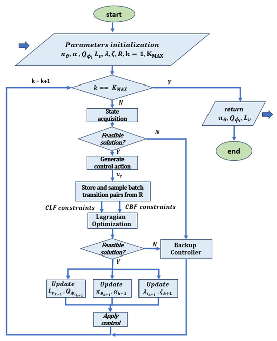 Figure 3. Flow chart related to the SAC algorithm, based on [40]. After initializing all networks, the neural controller , the Lyapunov function , the action-value networks with i = {1,2}, the Lagrange multipliers and , and the coefficient , the system applies a control signal and receives feedback, including reward and cost. The received transitions are stored in the replay buffer R and a set of transition pairs is randomly selected to construct the CBF and CLF constraints with the system f. These constraints are then used in RL controller training, where the extended Lagrangian method is used to update the parameters. If the safety and stability constraints are not satisfied, an optimal backup QP controller is designed to maintain basic safety.
- Deep deterministic policy gradient (DDPG): this is an actor–critic model-free algorithm that is based on the deterministic policy gradient and can operate over continuous action spaces. The goal is to learn the policy that maximizes the expected discounted cumulative long-term reward without violating the policy [59]. A flow chart of the method is reported in Figure 4.
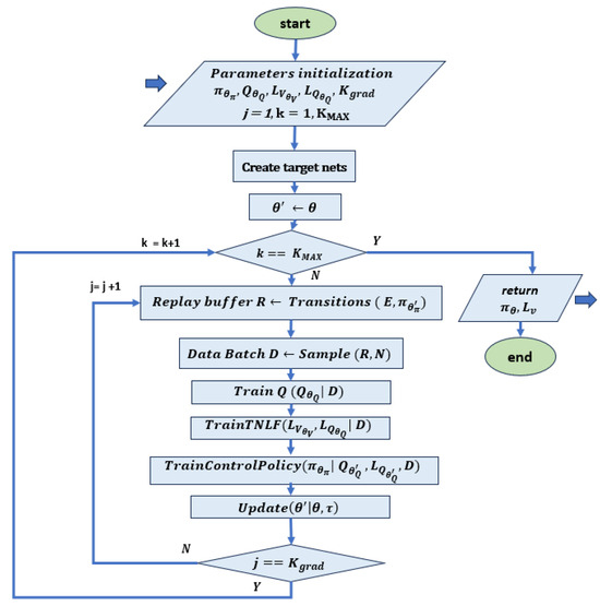 Figure 4. Flow chart related to the DDPG algorithm, based on [44]. This implementation is based on a co-learning framework where TNLF is trained together with the controller. The learning is based on the policy network , the Q-function network , their target networks and , the Lyapunov function network and the Lyapunov Q-function network . This acts as an additional critic for the actions of the actor, which is guided by its target network . The target networks are slowly changing networks that should follow the main value networks. After initializing the parameters, the transitions are sampled with the target network and the results are stored in the playback buffer R. This is normally used in RL to store the trajectories of experiences when executing a policy in an environment. Successively, the Q-net, the Lyapunov net and the respective target nets are trained on dataset D extracted from R. At the end of each step, the target networks are updated.
- Imitation learning (IL): this learning framework aims to acquire a policy that replicates the actions of experts who demonstrate how to perform the desired task. The expert’s behaviour can be encapsulated as a set of trajectories, where each element can come from different example conditions; furthermore, it can be both offline and online. It was used in [37] in combination with LMI formulation of stability condition, to synthesize a stable controller for an inverted pendulum and a car trajectory following. A flow chart of a typical IL approach is reported in Figure 5.
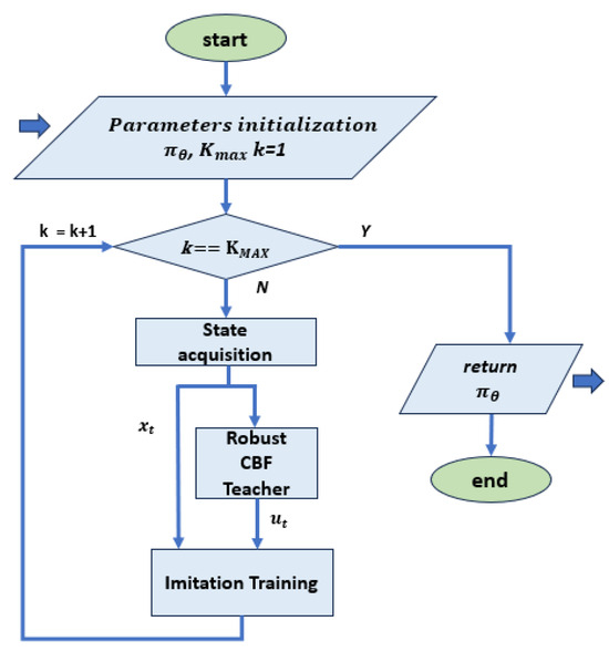 Figure 5. Flow chart for training with imitation learning, based on [35,37]. At each step, pairs of state values and control actions of the teacher controller are passed to the imitation training block as a reference. In this implementation, the teacher controller is based on an optimal controller that meets the safety conditions, so no further optimization block is required.
Other methods are worth mentioning that, even if they do not focus on finding stability features, have an impact on improving the motor skills of legged robots by utilising time-consuming offline iterations that preserve real-world robot training. In particular, Hwangbo et al. [60] presents a method for training a neural network policy in simulation and transferring it to a quadruped, which enables high-level speed commands and fall-recovery manoeuvres to be performed even in onboard experiments. The method was refined in [61] by developing a robust controller for quadruped locomotion in challenging natural environments that uses proprioceptive feedback and allows appropriate generalisation from the simulation to the real robot. The learned neural controller maintains the same robustness under conditions not encountered in training, such as deformable terrain and other examples of lifelike, wild outdoor areas. The method was extended in [62] with the integration of exteroceptive perception to combine the different perceptual modalities. The control was tested on a four-legged robot in different natural environments under various extreme weather conditions.
3.3. Linear and Nonlinear Programming
Linear and nonlinear programming (L&NP) refers to a large class of optimization problems where the objective functions can be linear or nonlinear (mostly quadratic) and the decision variables can be real, integer or binary numbers. A flow chart of a typical L&NP approach is reported in Figure 6. In view of the applications discussed in the following sections, the most important approaches are briefly presented below. Other approaches to certificate distillation or formalise the stability problem after a loop transformation and distil the associated Lyapunov function by LMI constraints [37] that have been proposed in the literature but are not detailed in this review are based on statistical learning methods (S) [42].
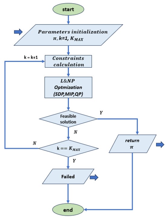
Figure 6.
Flow chart for training with NLP optimization, based on [46,47]. This diagram represents a general approach where the constraints are rewritten as specific optimization problems such as SDP, MIP or QP, which are evaluated with the corresponding software routines.
3.3.1. Quadratic Programming
An optimization problem with a quadratic objective function and linear constraints is called a quadratic program (QP). This can always be solved (or can be shown to be infeasible) in a finite number of iterations, but the effort required to find a solution depends strongly on the characteristics of the objective function and the number of inequality constraints. A general formulation is:
where is symmetric matrix, the index set I specifies the number of inequality constraints and and are vectors in [63].
A definition of a QP problem in terms of CLF/CBF function can be as follows:
where u is the control input, is a relaxation variable that ensures the solvability of QP as penalized by , and Q is any positive definite matrix. The certificate functions are expressed as inequality constraints in the overall QP problem, based on [26].
3.3.2. Mixed Integer Programming
A mixed integer programming (MIP) problem occurs when certain decision variables are restricted to integer values in the optimal solution. In this context, this formulation is used to check the Lyapunov stability conditions. In [13,34], a verifier is developed to test the positive and derivative Lyapunov stability conditions. To this purpose, the two conditions are rewritten as a mixed integer linear programming (MILP) problem, a special case of MIP, where the objective function, the bounds and the constraints are linear. To enable this evaluation, the plant, the controller and the relative cost function are expressed as an ANN with leaky ReLu activation functions. In [38], a verifier is obtained, but the evaluation is carried out through a mixed integer quadratic problem (MIQP), in which a quadratic term is used to synthesize the verifier.
3.3.3. Semi Definite Programming
Semidefinite programming (SDP) is a subfield of convex programming, where, in addition, the constraint matrix has to be positive semidefinite. A general form of SDP is given by:
where is a linear matrix inequality (LMI) and is a weight vector [64]. In [37], it is used to describe the LMI that combines Lyapunov theory with local quadratic constraints that limit the nonlinear activation functions in the ANN.
4. Applications
Lyapunov’s theory allows the formulation of methods based on CLF and CBF and is able to ensure stability and safety in the synthesis of control systems, even in the presence of disturbances and uncertainties. The different methods proposed in the literature have been evaluated in different case studies, which we can classify according to increasing levels of difficulty. The simplest applications concern the control of the inverse pendulum and trajectory tracking; where we have systems with small dimensions (few state variables), a limited number of constraints and easily linearizable models. A second category of applications concerns the control of drones, where a potentially larger number of variables are involved. Finally, applications investigating legged robots were considered, which have a high degree of complexity, both in terms of the number of state variables/constraints involved, and the models used, which often have to take into account the hybrid nature of such systems (due to the alternation of stance and swing phases in each leg). The most frequently considered robotic systems are bipeds and quadrupeds. As already mentioned, applications for legged robots are of primary interest in this review. The scenarios investigated concern locomotion control, posture and speed control, and navigation problems in which the robot must reach a target position in an environment with obstacles. Scenarios related to walking in environments with stepping stones are also considered, where precise positioning of the robot’s feet is required. All these applications were carried out both in simulated environments and with real robots in scenarios limited to 2D or extended to 3D. In Table 2, several case studies from the recent literature are listed, indicating the methodology used, the type of robot involved and the task involved. It is also indicated whether the applications were limited to simulations or extended to experimental tests with the robot. Examples of applications on quadruped and biped robots are shown in Figure 7. The different case studies are described below categorised according to the methodology used (i.e., CLF, CBF, CLBF).
Table 2.
Analysis of the CLF and CBF applications to walking robots: referred papers are check marked (✓) in terms of certificate type. Task, robot configuration and implementation type (simulation or real experiment) are also outlined.

Figure 7.
Application examples for four-legged and two-legged architectures. (a) LF on an 8-DoF quadruped robot controlled with a DDPG algorithm [44] to navigate towards a target location, in an environment filled with obstacles. (b) CBF with episodic learning on AMBER-3M biped controlled to walk on stepping stones, the time evolution of the barrier function at episode 0 [45] is reported in the panel where the distance between the robot feet and the stone centres is depicted. (c) LF on A1 quadruped with SAC algorithm for velocity tracking. The comparison between desired forward velocity and measured robot speed is reported in the panel [12]. (d) CBLF on DURUS 23-DoF biped with QP optimization for walking control on steps [50].
4.1. LF/CLF Applications
The impulsive nature of walking is at the basis of the strategy that models legged robots as hybrid systems. The problem of exponentially stabilizing periodic orbits in a special class of hybrid models was addressed in [43] using CLF. The proposed solution based on a variant of CLF that enforces rapid exponential convergence to the zero dynamics surface was illustrated on a hybrid model of a bipedal walking robot named RABBIT [66] through simulations and subsequently on the robotic testbed MABEL [67]. The CLF-based controller achieved a stable walking gait reducing undesirable oscillations in the presence of torque limits in the motors.
Algorithms designed to synthesize certificate functions often necessitate a closed-form analytical expression of the underlying dynamics. To overcome this constraint, algorithms capable of learning certificate functions solely from trajectory data have been proposed in [42]. The authors established the consistency of the learning process, illustrating its increasing accuracy with the expansion of the dataset size. The research involves the computation of upper bounds on the volume of violating regions, demonstrating their convergence to zero while the dataset increases in size. The generalization error of the learned certificate has been numerically estimated. An upper confidence bound (UCB) of the estimate has been performed using the Chernoff inequality. Empirical experiments have been performed using a damped pendulum as a simple example and a stable standing task with a quadruped robot named Minitaur subject to external forces [68]. The data acquisition was performed using PyBullet as a dynamic simulation environment [69]. A discrete-time Lyapunov function for handling the discontinuities in the trajectories due to contact forces has been trained and then tested using 10,000 trajectories. The median generalization UCB obtained was in the range of around 1–2%.
A novel cost-shaping method aimed at reducing the number of samples required to learn a stabilizing controller has been proposed in [12]. The method incorporates a CLF term into typical cost formulations to be used in Infinite Horizon RL strategies. The new cost functions result in stabilizing controllers when smaller discount factors are employed. The discount factor balances the importance of immediate versus future rewards. In principle, the smaller the value, the higher the weight of actual reward versus future ones and the simpler the problem to solve. Additionally, the inclusion of the CLF term ensures that even highly sub-optimal policies can stabilize the system. The authors illustrate their approach with two hardware examples: a cart pole and a quadruped robot using fine-tuning data acquired in only a few seconds and a few minutes of experiments, respectively. In particular, the Unitree A1 quadruped robot [70] was selected as a test bed to learn a neural network controller for velocity tracking. A nominal model-based controller proposed in [71] was used as the base system. Using a linearised reduced-order model, a CLF was designed around the desired robot gait. Using the data acquired from the robot, an RL algorithm was performed to learn a policy able to improve the velocity tracking performance of the base controller using only 5 min of robot data.
The quadruped robot was then loaded with an unknown load and a CLF was used to significantly decrease the tracking error of more than 60% using only one minute of robot data. Another hardware platform was used to validate the methodology: a linear servo base unit with an inverted pendulum (i.e., a Quanser cartpole system). Starting from the simulation-based policy, a CLF was synthesized for the underactuated system. The CLF-based fine-tuning approach was able to solve the swing-up task using data coming from a single rollout whereas multiple rollout data succeeded in learning a controller robust enough to recover from external pushes.
The controller developed in [43] for a bipedal walking robot was also fine-tuned. Model uncertainty was introduced on the mass of each robot link that was doubled. The nominal controller fails to stabilize the gait whereas only 40 s of data were enough to learn a CLF reducing the average tracking error. Moreover, a simulated inverted pendulum was also analyzed in the presence of input constraints. The addition of the candidate CLF in the reward allowed us to rapidly learn a stabilizing controller for different input bounds.
In the field of model-free deep RL used to solve high-dimensional problems in the presence of unknown dynamics, there is a strong need for safety assurance. In contrast with other approaches encoding safety constraints with rewards [12], the possibility to learn a twin neural Lyapunov function (TNLF) with the control policy in an RL framework was exploited in [44]. The TNLF works as a monitor to select the waypoints that guide the learned controller in combination with the path provided by a planner. The applications proposed refer to high-dimensional safety-sensitive navigation tasks where collision-free control trajectories are needed. Experiments were performed in a simulation environment optimized for reinforcement learning strategies (i.e., Safety Gym environment provided by OpenAI [72]). Robots with increasing levels of complexity were considered, including quadruped robots. This was torque-controlled at the hip and knee joints, providing state information from the joints, accelerometer, gyroscope, magnetometer, velocimeter, and a 2D vector toward the goal. The obstacle avoidance and target retrieving task was performed in terrains with different complexities, showing an improved success rate when the co-learning (i.e., TNFL and RL) strategy was adopted.
In [52], the authors propose an approach involving RoA-based planning methods to stabilize hybrid systems by using the RoA concept. The proposed method is to control the state of the system so that it always transitions to the RoA of the next hybrid mode after a change. The stability in each mode is ensured by using Lyapunov functions, and the RoA is represented by the invariant set provided by the Lyapunov function. Consequently, the system does not need to be optimized. This approach proves to be more effective in performing stability analysis and synthesizing controllers. A simulated bipedal robot with a compass gait was used as a test considering a QP controller for the low-level motion and a RoA classifier to find the optimal configuration imposed by the reference gait.
4.2. BF/CBF Applications
The generation of smooth paths that satisfy the dynamic constraints of walking robots is the topic discussed in [47]. The introduction of CBFs with path planning algorithms like rapidly exploring random trees (RRT/RRT*) was adopted to synthesize feasible collision-free paths dynamically. Logistic regression was used to represent arbitrarily shaped obstacles. A polynomial barrier function was derived from a grid map of the environment. The proposed CBF-RRT* algorithm was first validated in simulation with a dual-drive model and then experimentally with a 3D humanoid robot named Digit [73]. The algorithm found relatively optimal paths within 15 s and 40 interactions and was able to generate a collision-free path through complex spaces with polynomial-shaped obstacles.
Episodic learning and CBFs are combined for bipedal locomotion in [45] to achieve safety, defined in terms of set invariance. Here, a learning strategy has been implemented to mitigate the effects of model uncertainties that are relevant when considering hardware platforms, especially bipedal robots. The effects of system perturbations are directly reflected in a variation in the temporal derivative of the CBF, which is defined as a projected perturbation. Safety therefore implies a larger invariant set, which grows with the disturbance norm. Projection-to-state safety integrated with a machine learning framework was used to learn the model uncertainty as it affects the barrier functions. Projected disturbance is learned and hosted into an optimization-based controller. The strategy was evaluated both in simulation and on hardware using the bipedal AMBER-3M robot [74] modelled as an underactuated planar five-link robot with point feet dealing with a stepping stone problem. Stepping stones were modelled as squares of 8 cm in width. The CBF-QP provided a maximum barrier violation of 9.2 cm due to model uncertainties, which sometimes could cause the robot to fall. The use of a projected disturbance learning algorithm for two episodes, reduced the maximum barrier violation to 1.9 cm.
Episodic learning is also used in [53], where a method called Neural Gait is used to learn walking movements that are constrained within an invariant set and use experimental data episodically. Set invariance is achieved by CBF, which is defined on the zero dynamics and refers to the underactuated components of the robot. Although the input action does not directly influence the zero dynamics, it is indirectly influenced by the training parameters that are included in the CBF definition. The approach uses two learning structures. The first is dedicated to learning the walking gaits that minimise the violation of set invariance: it is designed using control-theoretic conditions for the barrier function. The latter learns episodically to minimise the discrepancies between the nominal model-based dynamics and the running hardware experiment. The AMBER-3M prototype is used as a demonstrator to show the efficiency of the approach in the presence of significant model discrepancies. The walking behaviour is described as a forward invariance set defined as a barrier satisfiability problem. In particular, a set of barrier functions is defined for the zero-dynamics subset. The overall strategy is trained to minimise the barrier conditions in the state space. To minimise model discrepancies, the residual error is trained on the zero dynamics and the corresponding correction is used to episodically refine the actual strategy and maximise the walking performance.
Dynamic locomotion over uneven terrains is a complex task. To simultaneously achieve safe foot placement and dynamic stability, a multi-layered locomotion architecture unifying CBFs with model predictive control (MPC) was proposed in [46] to assure both safety and longer horizon optimality. A control law designed without considering the safety issue could result in too aggressive actions next to the boundary of the safe region. The authors adopted CBF-based safety constraints both in a kinematic/dynamic formulation of the MPC low-frequency and in an inverse dynamics tracking controller working at high-frequency. The method was validated in a 3D stepping stone scenario both in simulation and experimentally on the ANYmal quadruped platform [75]. Walking in a stepping stone scenario, requiring precise foot placement, was considered. Simulation and robot experiments demonstrated that adopting CBF constraints on both the MPC and QP tracking layer outperforms other solutions that enforce CBF constraints at only one layer. In [65], a trajectory tracking control was developed to ensure safety in the presence of complex geometric elements in the environment modelled as polyhedra. The corresponding CBF, called the polygonal cone control barrier function (PolyC2BF), updates the concept of cone control barrier function proposed in [76]. The basic formulation of the CBF was carried out as a QP problem, where the function takes into account the vector between the centre of mass of the specific robot navigating through the environment and the centre of the obstacle it has to avoid, as well as the relative velocity and angle between these two vectors. It was tested on quadrupeds and a drone on Pybullet. In both cases, constant target velocities were chosen to validate the PolyC2BF.
In [36], a hybrid CBF (HCBF) was synthesized for a compass passive bipedal robot walking down an inclined plane at a constant velocity. In the walker, the initial state of the stance leg is fixed to the passive limit cycle and the initial state of the swing leg is varied by adding uniform noise to the corresponding passive limit cycle state. In this case, an energy-based controller was used as a teacher. The HCBF is described as an ANN with a fully connected neural network with two hidden layers with tanh activations and with 32 and 16 neurons in the first and second hidden layers, respectively, where the hyperparameters are determined by grid search. The obtained results demonstrated the presence of regions in the state space where the HCBF-based controller provides safe system trajectories while the energy-based controller results in unsafe behaviours.
4.3. CBLF Applications
Model uncertainty in safety-critical control is a relevant problem that can be treated using data-driven approaches. To handle this issue, an input-output linearization controller based on a nominal model was integrated with CLF and CBF in a QP problem using reinforcement learning techniques to deal with the model and constraints uncertainty [51]. The performance was validated on a planar five-link underactuated bipedal robot (i.e., RABBIT [66]) walking on a discrete terrain of randomly spaced stepping stones with a one-step preview. Stable and safe walking behaviours were obtained also under model uncertainty, changing the torso weight in the range [43 kg, 72 kg].
The design of CBFs can be facilitated following consolidated strategies as performed in [48] where a backstepping-inspired approach was considered. The method allows the generation of CBFs that guarantee forward invariance in a given set. The integration of safety constraints and control objectives through CLF-CBF-based QPs was also discussed. The method was validated on a walking task using the simulated seven-link bipedal robot, AMBER2 [77] where joint constraints are considered as CBFs, allowing the generation of stable walking. It should be noted that the authors in this paper use an earlier formulation of CBF, now referred to as reciprocal barrier function [26], which has the disadvantage that it grows infinitely towards the edge of the considered safe set, whereas the actual definition is preferable, as it can also be handled outside of this set.
Safety-critical control for nonlinear discrete-time systems was investigated in [49] using CBF in the discrete-time domain. Continuous-time formulations of CBF are applied to discrete-time systems through a nonlinear program that can be revised as a quadratically constrained quadratic program under certain hypotheses. The combination of discrete-time CLF and CBF was investigated. The method was applied to navigation control tasks using a 21-degree-of-freedom bipedal robot walking on a given path in environments with moving obstacles determining time-varying safety-critical constraints.
A single optimization-based controller was proposed in [50] to combine CLF to achieve periodic walking and CBF to impose constraints on step length and step width. The strategy was validated on the 3D humanoid robot DARUS [78] characterized by 23 degrees of freedom. The accomplished task was to demonstrate dynamic walking over stepping stones. Results demonstrated that the synthesized controller was able to handle random step length variations of about 30% of the nominal step length and random step width variations between 13% and 43% of the nominal step width.
5. Future Perspectives
In the field of learning control systems for walking robots, this review has identified promising methods that still need to be explored in the future for the control of walking robots. In addition to the already presented methods for synthesizing stability and safety certificates already used in legged robot scenarios, other promising approaches can be considered. In [13], a generic method for synthesizing a Lyapunov-stable neural network controller together with a neural-network-based Lyapunov function to simultaneously certify its stability was proposed. The problem was addressed in the context of MILP. Two algorithms were proposed: training the controller/Lyapunov function on training sets created by a verifier or using min-max optimization. Applications were performed with simulated robots, including a 2D and a 3D quadrotor. The controller for the 2D quadrotor, based on the model presented in [79], was trained with 10,000 initial states generated uniformly in the state space region under consideration. The results showed that the LQR controller was outperformed by the neural networks trained with CLF-based strategies. The convergence time ranged from 20 min to one day. The 3D quadrotor model with 12 state variables [80] was trained to perform a steering and hovering task obtaining a suitable controller in a few days. This methodology could be extended to legged robot control applications. In [29], approximate Lyapunov functions of dynamical systems in high dimensions were synthesized using an ANN. In this case, a —accurate Lyapunov (or control Lyapunov) function could be derived: the model guarantees positive definiteness and is trained to fulfil the negative orbital derivative condition, leading to only one term in an empirical risk function. Minimizing this simple risk function allows for less manual tuning of hyperparameters and more efficient optimization. Experimental results have been performed with 2D systems for curve tracking, but also with 10D and 30D synthetic systems and for the evaluation of the attraction region of an inverted pendulum. Based on this perspective, it should be quite straightforward to adapt the method for applications involving legged systems. While the empirical performance of existing techniques is remarkable under certain conditions, the critical drawback of ensuring safety and stability in more general cases requires innovative approaches. The following future perspectives indicate possible directions to advance the field:
- Data-efficient Lyapunov functional distillation: Addressing the challenges related to the availability and efficiency of datasets for Lyapunov function distillation is crucial [42]. Future research should focus on methods that improve the extraction of Lyapunov functions from limited datasets to ensure robustness and efficiency in learning-based control systems.
- Integration of Lyapunov design techniques with offline learning: The current review highlights the potential of Lyapunov design techniques in reinforcement learning, especially in offline environments [12]. Future efforts could explore and extend the integration of Lyapunov-based approaches with reinforcement learning to achieve robust and efficient control policies in legged robotic systems.
- Flexible approaches based on system requirements: Depending on the specific requirements of a given system, future research could look at flexible approaches that combine CLFs and CBFs based on the priorities of stability or constraint satisfaction [81]. This adaptability ensures that control strategies can be tailored to the specific needs of different robotic systems, including a grading in the level of certification that can be relaxed when the robot generalizes the trained task, trying to extend the safety region beyond that one related to the training dataset.
- Terrain adaptation and obstacle avoidance: A major challenge for legged robots is to navigate uneven and discrete (rocky) terrains while avoiding obstacles [3]. Future work should aim to implement and further integrate discrete-time CBFs with continuous-time controllers to improve the adaptability and obstacle-avoidance capability of legged robots [45,49].
- Development of standard benchmarks: The development of standard benchmarks for the application of legged robots plays a critical role in the advancement of robotics by providing a common framework for evaluating control strategies. Standard benchmarks serve as important tools for evaluating the performance, robustness and adaptability of different control algorithms for different legged-robot platforms. These benchmarks will facilitate fair and objective comparisons between different control strategies, promote healthy competition and accelerate the identification of best practices. The introduction of benchmarks also encourages knowledge sharing and collaboration within the scientific community, as researchers can collectively contribute to the refinement and expansion of these standardized tests.
In summary, the future of adaptive control systems for legged robots offers exciting opportunities driven by the integration of innovative methods and the pursuit of multi-level performance guarantees. These future prospects aim to overcome current limitations and push the field towards safer, more adaptive and more efficient legged robotic systems.
6. Conclusions
This review addresses the critical challenge of providing stability and safety guarantees for learning control systems, with a focus on walking robots such as bipeds and quadrupeds. While learning-based control systems have shown impressive performance in practice, the lack of safety and stability guarantees is a significant drawback. This review highlights the growing importance of stability certification techniques that combine learning certificates with control strategies to ensure safety during training and verification after training.
The focus is on legged robots, which are becoming increasingly popular due to their dexterity and ability to navigate unstructured terrains. The need for stability guarantees is critical as these robots are used in applications where traditional wheeled robots reach their limits. Legged robots that move with articulated limbs pose particular challenges to dynamic stability due to the complexity of their bodies and the constraints imposed by contact forces and actuation limits.
The article reviews the current state of the art in the development of stability and barrier functions, focusing on Control Lyapunov Functions and Control Barrier Functions. Data-driven techniques are also discussed, with a focus on neural networks, and applications to walking robots are explored. The importance of reinforcement learning in providing stability and safety guarantees is emphasized, especially in real-time applications where hardware implementation challenges arise. The authors emphasize the relevance of learning with the addition of stability and safety certificates, which provide a reliable method to control and improve learning processes. The integration of these certificates into the learning paradigm ensures more reliable and robust solutions. Different learning strategies were considered such as supervised approaches, reinforcement learning algorithms and several linear and nonlinear programming techniques (i.e., QP, MIP, SDP, and others). Furthermore, the potential impact on real-time control strategies is discussed, where neural controllers shift the computational load to the offline training phase, enabling efficient performance during operation. The analyzed applications in the field of legged robots address different relevant tasks that include: stable standing, velocity tracking, locomotion control, walking on stepping stones and navigation control. These tasks are evaluated on several different legged robots both in simulation and real scenarios.
Future perspectives are finally presented, underlying the importance of several aspects that contribute to achieving the common objective of developing control systems with safety and stability guarantees to be applied to robotic systems working in real-world scenarios. The underlined future research directions range from data-efficient solutions, online and offline learning integration, flexibility in the imposed constraints, generalization capabilities and the development of standard benchmarks to facilitate the performance evaluation.
Author Contributions
Conceptualization, methodology, software, investigation, and writing: L.P., A.L.N. and P.A.; Conceptualization, supervision, writing—review and editing: L.P., A.L.N. and P.A.; Supervision and project administration: L.P. and P.A. All authors have read and agreed to the published version of the manuscript.
Funding
The work was supported by MUR PNRR—Mission 4-Comp.2—Inv:1.3—project PE0000013-FAIR.
Data Availability Statement
The data presented in this study are available on request from the corresponding author.
Conflicts of Interest
The authors declare no conflicts of interest.
References
- Prajna, S.; Jadbabaie, A. Safety Verification of Hybrid Systems Using Barrier Certificates. In Proceedings of the International Conference on Hybrid Systems: Computation and Control, Philadelphia, PA, USA, 25–27 March 2004. [Google Scholar]
- Prajna, S. Barrier certificates for nonlinear model validation. Automatica 2006, 42, 117–126. [Google Scholar] [CrossRef]
- Torres-Pardo, A.; Pinto-Fernández, D.; Garabini, M.; Angelini, F.; Rodriguez-Cianca, D.; Massardi, S.; Tornero, J.; Moreno, J.C.; Torricelli, D. Legged locomotion over irregular terrains: State of the art of human and robot performance. Bioinspir. Biomim. 2022, 17, 061002. [Google Scholar] [CrossRef] [PubMed]
- Bouman, A.; Ginting, M.F.; Alatur, N.; Palieri, M.; Fan, D.D.; Touma, T.; Pailevanian, T.; Kim, S.K.; Otsu, K.; Burdick, J.; et al. Autonomous Spot: Long-Range Autonomous Exploration of Extreme Environments with Legged Locomotion. In Proceedings of the 2020 IEEE/RSJ International Conference on Intelligent Robots and Systems (IROS), Las Vegas, NV, USA, 24 October 2020–24 January 2021; pp. 2518–2525. [Google Scholar] [CrossRef]
- Arena, P.; Patanè, L.; Taffara, S. A Data-Driven Model Predictive Control for Quadruped Robot Steering on Slippery Surfaces. Robotics 2023, 12, 67. [Google Scholar] [CrossRef]
- Patané, L. Bio-inspired robotic solutions for landslide monitoring. Energies 2019, 12, 1256. [Google Scholar] [CrossRef]
- Arena, P.; Patanè, L.; Taffara, S. Learning risk-mediated traversability maps in unstructured terrains navigation through robot-oriented models. Inf. Sci. 2021, 576, 1–23. [Google Scholar] [CrossRef]
- Semini, C.; Wieber, P.B. Legged Robots. In Encyclopedia of Robotics; Springer: Berlin/Heidelberg, Germany, 2020; pp. 1–11. [Google Scholar] [CrossRef]
- Ren, Z.; Lai, J.; Wu, Z.; Xie, S. Deep neural networks-based real-time optimal navigation for an automatic guided vehicle with static and dynamic obstacles. Neurocomputing 2021, 443, 329–344. [Google Scholar] [CrossRef]
- Singh, N.; Thongam, K. Neural network-based approaches for mobile robot navigation in static and moving obstacles environments. Intell. Serv. Robot. 2019, 12, 55–67. [Google Scholar] [CrossRef]
- Xiao, W.; Cassandras, G.C.; Belta, C. Safety-Critical Optimal Control for Autonomous Systems. J. Syst. Sci. Complex. 2021, 34, 1723–1742. [Google Scholar] [CrossRef]
- Westenbroek, T.; Castaneda, F.; Agrawal, A.; Sastry, S.; Sreenath, K. Lyapunov Design for Robust and Efficient Robotic Reinforcement Learning. arXiv 2022, arXiv:2208.06721. [Google Scholar]
- Dai, H.; Landry, B.; Yang, L.; Pavone, M.; Tedrake, R. Lyapunov-stable neural-network control. arXiv 2021, arXiv:2109.14152. [Google Scholar]
- Dawson, C.; Gao, S.; Fan, C. Safe Control With Learned Certificates: A Survey of Neural Lyapunov, Barrier, and Contraction Methods for Robotics and Control. IEEE Trans. Robot. 2022, 39, 1749–1767. [Google Scholar] [CrossRef]
- Hafstein, S.; Giesl, P. Computational methods for Lyapunov functions. Discret. Contin. Dyn. Syst. Ser. B 2015, 20, i–ii. [Google Scholar] [CrossRef]
- Tsukamoto, H.; Chung, S.J.; Slotine, J.J.E. Contraction theory for nonlinear stability analysis and learning-based control: A tutorial overview. Annu. Rev. Control 2021, 52, 135–169. [Google Scholar] [CrossRef]
- Anand, A.; Seel, K.; Gjaerum, V.; Haakansson, A.; Robinson, H.; Saad, A. Safe Learning for Control using Control Lyapunov Functions and Control Barrier Functions: A Review. Procedia Comput. Sci. 2021, 192, 3987–3997. [Google Scholar] [CrossRef]
- Hu, K.; Ott, C.; Lee, D. Online iterative learning control of zero-moment point for biped walking stabilization. In Proceedings of the 2015 IEEE International Conference on Robotics and Automation (ICRA), Seattle, WA, USA, 26–30 May 2015; pp. 5127–5133. [Google Scholar]
- Hu, K.; Ott, C.; Lee, D. Learning and Generalization of Compensative Zero-Moment Point Trajectory for Biped Walking. IEEE Trans. Robot. 2016, 32, 717–725. [Google Scholar] [CrossRef]
- Cybenko, G. Approximation by superpositions of a sigmoidal function. Math. Control Signals Syst. 1989, 2, 303–314. [Google Scholar] [CrossRef]
- Elallid, B.B.; Benamar, N.; Hafid, A.S.; Rachidi, T.; Mrani, N. A Comprehensive Survey on the Application of Deep and Reinforcement Learning Approaches in Autonomous Driving. J. King Saud Univ. Comput. Inf. Sci. 2022, 34, 7366–7390. [Google Scholar] [CrossRef]
- Xie, J.; Shao, Z.; Li, Y.; Guan, Y.; Tan, J. Deep Reinforcement Learning with Optimized Reward Functions for Robotic Trajectory Planning. IEEE Access 2019, 7, 105669–105679. [Google Scholar] [CrossRef]
- Khalil, H.K. Nonlinear Systems, 3rd ed.; Prentice-Hall: Upper Saddle River, NJ, USA, 2002. [Google Scholar]
- Nagumo, M. Über Die LAGE der Integralkurven Gewöhnlicher Differentialgleichungen. 1942. Available online: https://www.jstage.jst.go.jp/article/ppmsj1919/24/0/24_0_551/_pdf (accessed on 1 November 2023).
- Prajna, S.; Jadbabaie, A. Safety Verification of Hybrid Systems Using Barrier Certificates. In Hybrid Systems: Computation and Control; Alur, R., Pappas, G.J., Eds.; Springer: Berlin/Heidelberg, Germany, 2004; pp. 477–492. [Google Scholar]
- Ames, A.; Coogan, S.D.; Egerstedt, M.; Notomista, G.; Sreenath, K.; Tabuada, P. Control Barrier Functions: Theory and Applications. In Proceedings of the 2019 18th European Control Conference (ECC), Naples, Italy, 25–28 June 2019; pp. 3420–3431. [Google Scholar]
- Dawson, C.; Qin, Z.; Gao, S.; Fan, C. Safe Nonlinear Control Using Robust Neural Lyapunov-Barrier Functions. arXiv 2021, arXiv:2109.06697. [Google Scholar]
- Richards, S.; Berkenkamp, F.; Krause, A. The Lyapunov Neural Network: Adaptive Stability Certification for Safe Learning of Dynamical Systems. In Proceedings of the 2nd Conference on Robot Learning (CoRL 2018), Zurich, Switzerland, 29–31 October 2018. [Google Scholar]
- Gaby, N.; Zhang, F.; Ye, X. Lyapunov-Net: A Deep Neural Network Architecture for Lyapunov Function Approximation. arXiv 2022, arXiv:2109.13359. [Google Scholar]
- Abate, A.; Ahmed, D.; Giacobbe, M.; Peruffo, A. Formal Synthesis of Lyapunov Neural Networks. IEEE Control Syst. Lett. 2021, 5, 773–778. [Google Scholar] [CrossRef]
- Abate, A.; Ahmed, D.; Edwards, A.; Giacobbe, M.; Peruffo, A. FOSSIL: A Software Tool for the Formal Synthesis of Lyapunov Functions and Barrier Certificates Using Neural Networks. In Proceedings of the 24th International Conference on Hybrid Systems: Computation and Control (HSCC ’21), New York, NY, USA, 19–21 May 2021. [Google Scholar] [CrossRef]
- Zhou, R.; Quartz, T.; Sterck, H.D.; Liu, J. Neural Lyapunov Control of Unknown Nonlinear Systems with Stability Guarantees. arXiv 2022, arXiv:2206.01913. [Google Scholar]
- Chang, Y.C.; Roohi, N.; Gao, S. Neural Lyapunov Control. arXiv 2022, arXiv:2005.00611. [Google Scholar]
- Wu, J.; Clark, A.; Kantaros, Y.; Vorobeychik, Y. Neural Lyapunov Control for Discrete-Time Systems. arXiv 2023, arXiv:2305.06547. [Google Scholar]
- Cosner, R.K.; Yue, Y.; Ames, A.D. End-to-End Imitation Learning with Safety Guarantees using Control Barrier Functions. arXiv 2022, arXiv:2212.11365. [Google Scholar]
- Lindemann, L.; Hu, H.; Robey, A.; Zhang, H.; Dimarogonas, D.V.; Tu, S.; Matni, N. Learning Hybrid Control Barrier Functions from Data. arXiv 2020, arXiv:2011.04112. [Google Scholar]
- Yin, H.; Seiler, P.; Jin, M.; Arcak, M. Imitation Learning with Stability and Safety Guarantees. arXiv 2021, arXiv:2012.09293. [Google Scholar] [CrossRef]
- Chen, S.; Fazlyab, M.; Morari, M.; Pappas, G.J.; Preciado, V.M. Learning Lyapunov Functions for Hybrid Systems. In Proceedings of the 2021 55th Annual Conference on Information Sciences and Systems (CISS), Baltimore, MD, USA, 24–26 March 2021; p. 1. [Google Scholar]
- Chow, Y.; Nachum, O.; Duenez-Guzman, E.; Ghavamzadeh, M. A Lyapunov-based Approach to Safe Reinforcement Learning. arXiv 2018, arXiv:1805.07708. [Google Scholar]
- Zhao, L.; Gatsis, K.; Papachristodoulou, A. Stable and Safe Reinforcement Learning via a Barrier-Lyapunov Actor–Critic Approach. arXiv 2023, arXiv:2304.04066. [Google Scholar]
- Hejase, B.; Ozguner, U. Lyapunov Stability Regulation of Deep Reinforcement Learning Control with Application to Automated Driving. In Proceedings of the 2023 American Control Conference (ACC), San Diego, CA, USA, 31 May–2 June 2023; pp. 4437–4442. [Google Scholar] [CrossRef]
- Boffi, N.M.; Tu, S.; Matni, N.; Slotine, J.J.E.; Sindhwani, V. Learning Stability Certificates from Data. arXiv 2020, arXiv:2008.05952. [Google Scholar]
- Ames, A.D.; Galloway, K.; Sreenath, K.; Grizzle, J.W. Rapidly Exponentially Stabilizing Control Lyapunov Functions and Hybrid Zero Dynamics. IEEE Trans. Autom. Control 2014, 59, 876–891. [Google Scholar] [CrossRef]
- Xiong, Z.; Eappen, J.; Qureshi, A.H.; Jagannathan, S. Model-free Neural Lyapunov Control for Safe Robot Navigation. In Proceedings of the 2022 IEEE/RSJ International Conference on Intelligent Robots and Systems (IROS), Kyoto, Japan, 23–27 October 2022; pp. 5572–5579. [Google Scholar]
- Csomay-Shanklin, N.; Cosner, R.K.; Dai, M.; Taylor, A.J.; Ames, A.D. Episodic Learning for Safe Bipedal Locomotion with Control Barrier Functions and Projection-to-State Safety. In Proceedings of the 3rd Conference on Learning for Dynamics and Control, Virtual Event, Switzerland, 7–8 June 2021; Jadbabaie, A., Lygeros, J., Pappas, G.J., Parrilo, P.A., Recht, B., Tomlin, C.J., Zeilinger, M.N., Eds.; PMLR: Maastricht, Germany, 2021; Volume 144, pp. 1041–1053. [Google Scholar]
- Grandia, R.; Taylor, A.J.; Ames, A.D.; Hutter, M. Multi-Layered Safety for Legged Robots via Control Barrier Functions and Model Predictive Control. In Proceedings of the 2021 IEEE International Conference on Robotics and Automation (ICRA), Xi’an, China, 30 May–5 June 2021; pp. 8352–8358. [Google Scholar] [CrossRef]
- Peng, C.; Donca, O.; Hereid, A. Safe Path Planning for Polynomial Shape Obstacles via Control Barrier Functions and Logistic Regression. arXiv 2022, arXiv:2210.03704. [Google Scholar]
- Hsu, S.C.; Xu, X.; Ames, A.D. Control barrier function based quadratic programs with application to bipedal robotic walking. In Proceedings of the 2015 American Control Conference (ACC), Chicago, IL, USA, 1–3 July 2015; pp. 4542–4548. [Google Scholar] [CrossRef]
- Agrawal, A.; Sreenath, K. Discrete Control Barrier Functions for Safety-Critical Control of Discrete Systems with Application to Bipedal Robot Navigation. In Proceedings of the Robotics: Science and Systems, Cambridge, MA, USA, 12–16 July 2017. [Google Scholar]
- Nguyen, Q.; Hereid, A.; Grizzle, J.W.; Ames, A.D.; Sreenath, K. 3D dynamic walking on stepping stones with Control Barrier Functions. In Proceedings of the 2016 IEEE 55th Conference on Decision and Control (CDC), Las Vegas, NV, USA, 12–14 December 2016; pp. 827–834. [Google Scholar] [CrossRef]
- Choi, J.J.; Castañeda, F.; Tomlin, C.J.; Sreenath, K. Reinforcement Learning for Safety-Critical Control under Model Uncertainty, using Control Lyapunov Functions and Control Barrier Functions. arXiv 2020, arXiv:2004.07584. [Google Scholar]
- Meng, Y.; Fan, C. Hybrid Systems Neural Control with Region-of-Attraction Planner. arXiv 2023, arXiv:2303.10327. [Google Scholar]
- Rodriguez, I.D.J.; Csomay-Shanklin, N.; Yue, Y.; Ames, A. Neural Gaits: Learning Bipedal Locomotion via Control Barrier Functions and Zero Dynamics Policies. In Proceedings of the Conference on Learning for Dynamics & Control, Stanford, CA, USA, 23–24 June 2022. [Google Scholar]
- Cunningham, P.; Cord, M.; Delany, S.J. Supervised Learning. In Machine Learning Techniques for Multimedia: Case Studies on Organization and Retrieval; Springer: Berlin/Heidelberg, Germany, 2008; pp. 21–49. [Google Scholar] [CrossRef]
- Barreto, G.; Araújo, A.; Ritter, H. Self-Organizing Feature Maps for Modeling and Control of Robotic Manipulators. J. Intell. Robot. Syst. 2003, 36, 407–450. [Google Scholar] [CrossRef]
- Arena, P.; Di Pietro, F.; Li Noce, A.; Patanè, L. Attitude control in the Mini Cheetah robot via MPC and reward-based feed-forward controller. IFAC-PapersOnLine 2022, 55, 41–48. [Google Scholar] [CrossRef]
- Yu, K.; Jin, K.; Deng, X. Review of Deep Reinforcement Learning. In Proceedings of the 2022 IEEE 5th Advanced Information Management, Communicates, Electronic and Automation Control Conference (IMCEC), Chongqing China, 16–18 December 2022; Volume 5, pp. 41–48. [Google Scholar] [CrossRef]
- Haarnoja, T.; Zhou, A.; Abbeel, P.; Levine, S. Soft Actor–Critic: Off-Policy Maximum Entropy Deep Reinforcement Learning with a Stochastic Actor. arXiv 2018, arXiv:1801.01290. [Google Scholar]
- Lillicrap, T.P.; Hunt, J.J.; Pritzel, A.; Heess, N.; Erez, T.; Tassa, Y.; Silver, D.; Wierstra, D. Continuous control with deep reinforcement learning. arXiv 2019, arXiv:1509.02971. [Google Scholar]
- Hwangbo, J.; Lee, J.; Dosovitskiy, A.; Bellicoso, D.; Tsounis, V.; Koltun, V.; Hutter, M. Learning agile and dynamic motor skills for legged robots. Sci. Robot. 2019, 4, eaau5872. [Google Scholar] [CrossRef]
- Lee, J.; Hwangbo, J.; Wellhausen, L.; Koltun, V.; Hutter, M. Learning quadrupedal locomotion over challenging terrain. Sci. Robot. 2020, 5, eabc5986. [Google Scholar] [CrossRef]
- Miki, T.; Lee, J.; Hwangbo, J.; Wellhausen, L.; Koltun, V.; Hutter, M. Learning robust perceptive locomotion for quadrupedal robots in the wild. Sci. Robot. 2022, 7, eabk2822. [Google Scholar] [CrossRef] [PubMed]
- Nocedal, J.; Wright, S.J. (Eds.) Quadratic Programming. In Numerical Optimization; Springer: New York, NY, USA, 1999; pp. 438–486. [Google Scholar] [CrossRef]
- Vandenberghe, L.; Boyd, S. Semidefinite Programming. SIAM Rev. 1996, 38, 49–95. [Google Scholar] [CrossRef]
- Tayal, M.; Kolathaya, S. Polygonal Cone Control Barrier Functions (PolyC2BF) for safe navigation in cluttered environments. arXiv 2023, arXiv:2311.08787. [Google Scholar]
- Westervelt, E.; Buche, G.; Grizzle, J. Experimental Validation of a Framework for the Design of Controllers that Induce Stable Walking in Planar Bipeds. I. J. Robot. Res. 2004, 23, 559–582. [Google Scholar] [CrossRef]
- Sreenath, K.; Park, H.W.; Poulakakis, I.; Grizzle, J. A Compliant Hybrid Zero Dynamics Controller for Stable, Efficient and Fast Bipedal Walking on MABEL. I. J. Robot. Res. 2011, 30, 1170–1193. [Google Scholar] [CrossRef]
- Kenneally, G.; De, A.; Koditschek, D.E. Design Principles for a Family of Direct-Drive Legged Robots. IEEE Robot. Autom. Lett. 2016, 1, 900–907. [Google Scholar] [CrossRef]
- Coumans, E.; Bai, Y. Pybullet, a Python Module for Physics Simulation for Games, Robotics and Machine Learning. 2020. Available online: https://docs.google.com/document/d/10sXEhzFRSnvFcl3XxNGhnD4N2SedqwdAvK3dsihxVUA (accessed on 1 November 2023).
- Unitree. A1 Quadruped Robot. 2023. Available online: https://m.unitree.com/a1/ (accessed on 1 November 2023).
- Da, X.; Xie, Z.; Hoeller, D.; Boots, B.; Anandkumar, A.; Zhu, Y.; Babich, B.; Garg, A. Learning a Contact-Adaptive Controller for Robust, Efficient Legged Locomotion. arXiv 2020, arXiv:2009.10019. [Google Scholar]
- Ray, A.; Achiam, J.; Amodei, D. Benchmarking safe exploration in deep reinforcement learning. arXiv 2019, arXiv:1910.01708. [Google Scholar]
- Castillo, G.A.; Weng, B.; Zhang, W.; Hereid, A. Robust Feedback Motion Policy Design Using Reinforcement Learning on a 3D Digit Bipedal Robot. In Proceedings of the 2021 IEEE/RSJ International Conference on Intelligent Robots and Systems (IROS), Prague, Czech Republic, 27 September–1 October 2021; pp. 5136–5143. [Google Scholar] [CrossRef]
- Ambrose, E.; Ma, W.L.; Hubicki, C.; Ames, A.D. Toward benchmarking locomotion economy across design configurations on the modular robot: AMBER-3M. In Proceedings of the 2017 IEEE Conference on Control Technology and Applications (CCTA), Kohala Coast, HI, USA, 27–30 August 2017; pp. 1270–1276. [Google Scholar] [CrossRef]
- Hutter, M.; Gehring, C.; Jud, D.; Lauber, A.; Bellicoso, C.D.; Tsounis, V.; Hwangbo, J.; Bodie, K.; Fankhauser, P.; Bloesch, M.; et al. ANYmal—A highly mobile and dynamic quadrupedal robot. In Proceedings of the 2016 IEEE/RSJ International Conference on Intelligent Robots and Systems (IROS), Daejeon, Republic of Korea, 9–14 October 2016; pp. 38–44. [Google Scholar] [CrossRef]
- Tayal, M.; Kolathaya, S.N.Y. Safe Legged Locomotion Using Collision Cone Control Barrier Functions (C3BFs). arXiv 2023, arXiv:2309.01898. [Google Scholar]
- Ma, W.L.; Zhao, H.H.; Kolathaya, S.; Ames, A.D. Human-inspired walking via unified PD and impedance control. In Proceedings of the 2014 IEEE International Conference on Robotics and Automation (ICRA), Hong Kong, China, 31 May–7 June 2014; pp. 5088–5094. [Google Scholar] [CrossRef]
- Reher, J.; Cousineau, E.A.; Hereid, A.; Hubicki, C.M.; Ames, A.D. Realizing dynamic and efficient bipedal locomotion on the humanoid robot DURUS. In Proceedings of the 2016 IEEE International Conference on Robotics and Automation (ICRA), Stockholm, Sweden, 16–21 May 2016; pp. 1794–1801. [Google Scholar] [CrossRef]
- Tedrake, R. Underactuated robotics: Learning, planning, and control for efficient and agile machines, Course notes for MIT, 6:832. Work. Draft. Ed. 2009, 3, 2. [Google Scholar]
- Mellinger, D.; Kumar, V. Minimum snap trajectory generation and control for quadrotors. In Proceedings of the 2011 IEEE International Conference on Robotics and Automation, Shanghai, China, 9–13 May 2011; pp. 2520–2525. [Google Scholar] [CrossRef]
- Jin, W.; Wang, Z.; Yang, Z.; Mou, S. Neural Certificates for Safe Control Policies. arXiv 2020, arXiv:2006.08465. [Google Scholar]

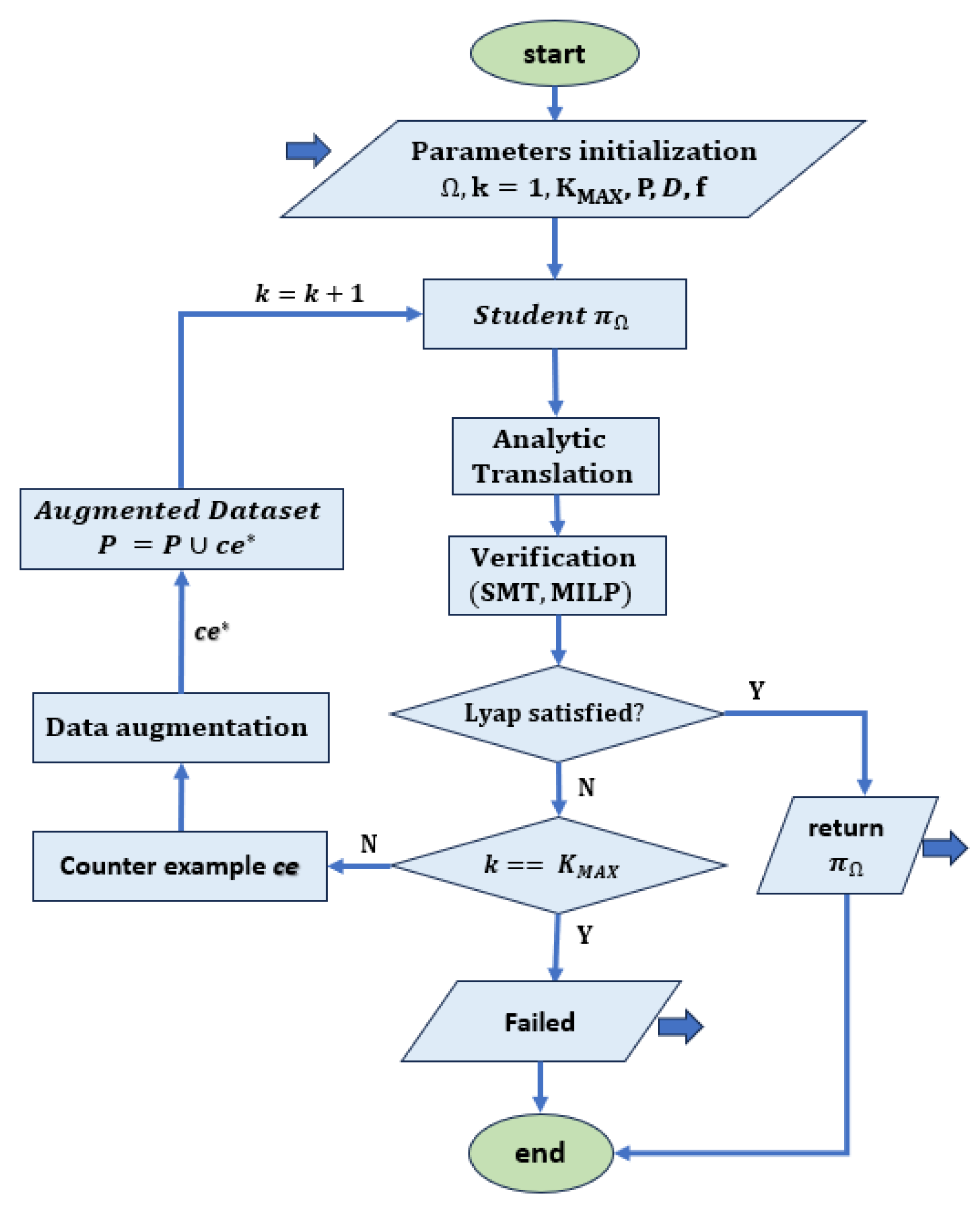

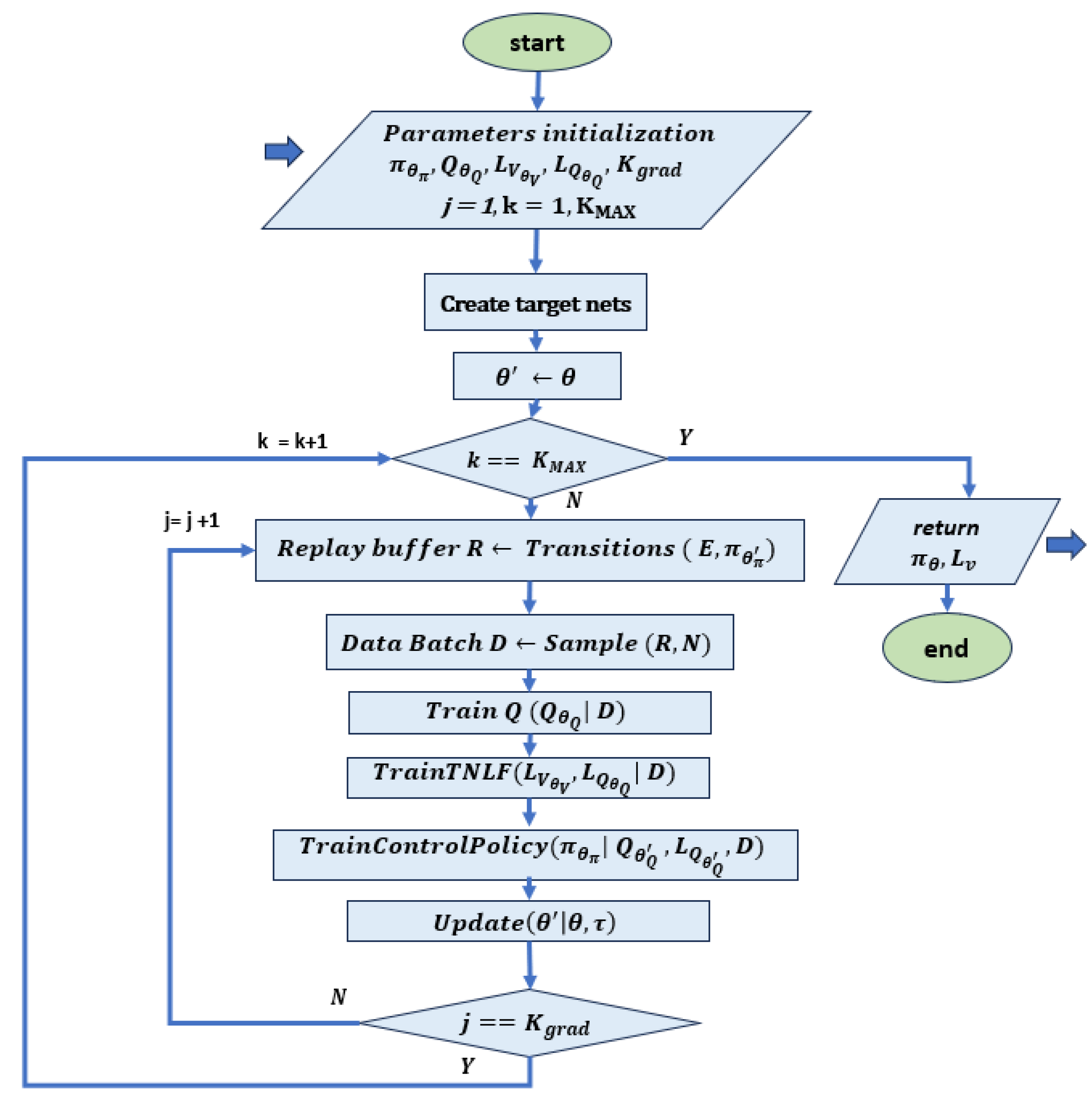

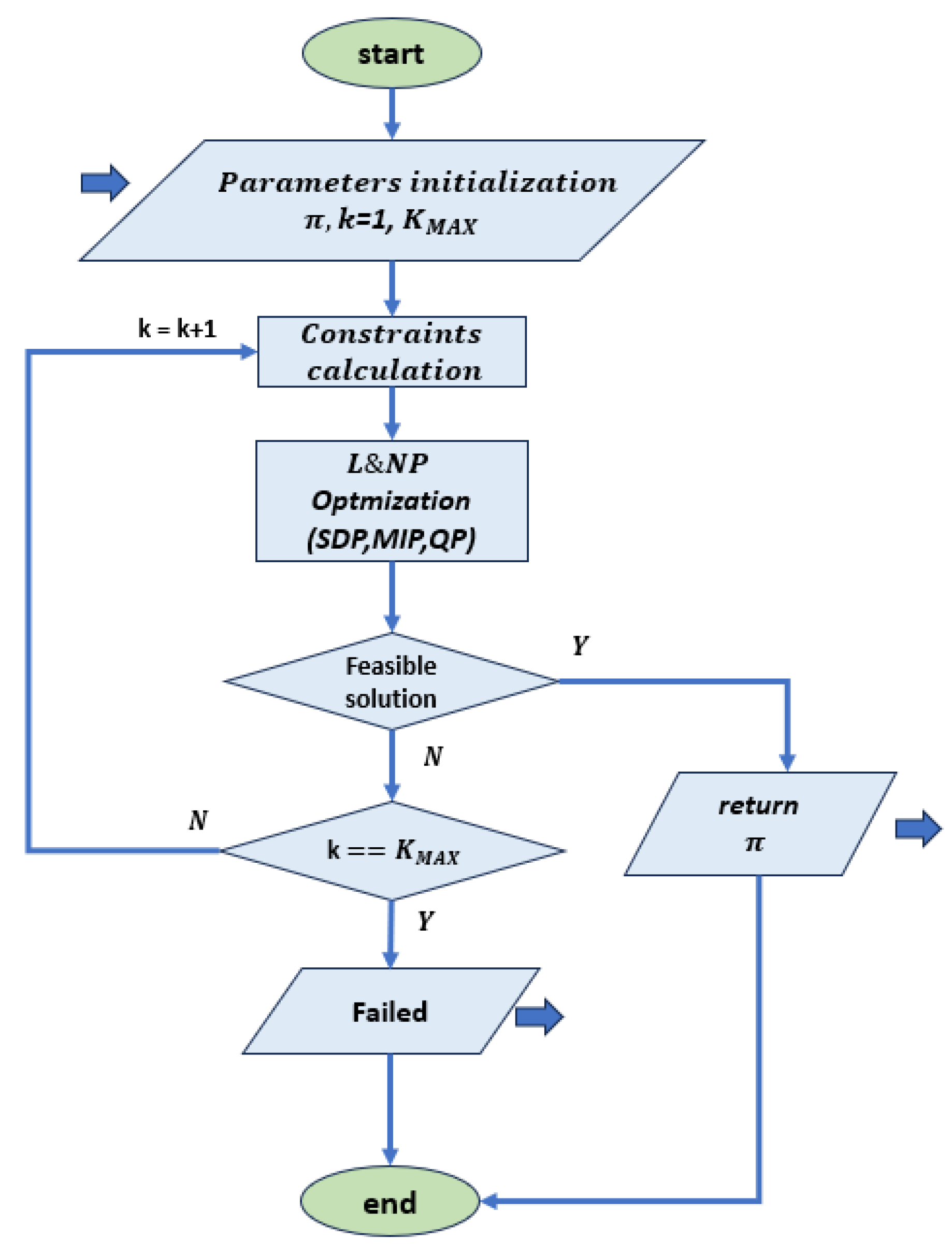
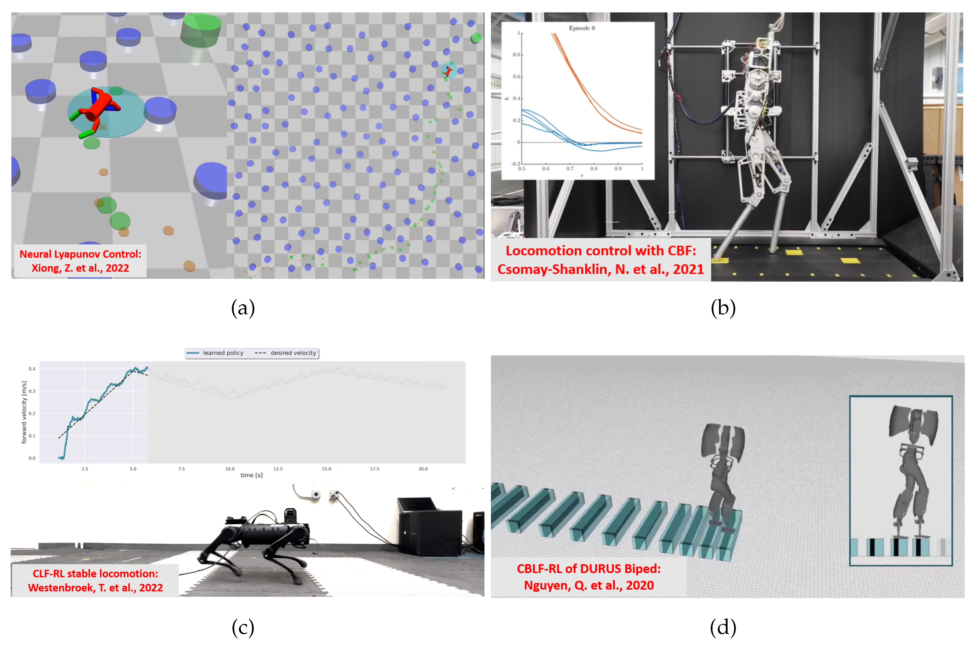
Disclaimer/Publisher’s Note: The statements, opinions and data contained in all publications are solely those of the individual author(s) and contributor(s) and not of MDPI and/or the editor(s). MDPI and/or the editor(s) disclaim responsibility for any injury to people or property resulting from any ideas, methods, instructions or products referred to in the content. |
© 2024 by the authors. Licensee MDPI, Basel, Switzerland. This article is an open access article distributed under the terms and conditions of the Creative Commons Attribution (CC BY) license (https://creativecommons.org/licenses/by/4.0/).