Experimental Nonlinear and Incremental Control Stabilization of a Tail-Sitter UAV with Hardware-in-the-Loop Validation

Abstract

Tail-sitters aim to combine the advantages of fixed-wing aircraft and rotorcraft but require a robust and fast stabilization strategy to perform vertical maneuvers and transitions to and from aerodynamic flight. The research conducted in this work explores different nonlinear control solutions for the problem of stabilizing a tail-sitter when hovering. For this purpose, the first controller is an existing strategy for tail-sitter control obtained from the literature, the second is an application of Nonlinear Dynamic Inversion (NDI), and the last one is its incremental version, INDI. These controllers were implemented and tuned in a simulation in order to stabilize a model of the tail-sitter, complemented by estimation methods that allow the feedback of the necessary variables. These estimators and controllers were then implemented in a microcontroller and validated in a Hardware-in-the-Loop (HITL) scenario with simple maneuvers in vertical flight. Lastly, the developed control solutions were used to stabilize the aircraft in experimental flight while being monitored by a motion capture system. The experimental results allow the validation of the model of the X-Vert and provide a comparison of the performance of the different control solutions, where the INDI presents itself as a robust control strategy with accurate tracking capabilities and less actuator demand.

1. Introduction

Unmanned Aerial Vehicles (UAVs) have been increasing in popularity in the last decades, with broad scientific, industrial and military uses [1]. From a wide range of urban applications [2] to topographic mapping and surveillance operations [3], which are useful for agricultural purposes [4], for example, these aircraft are undeniably helpful and are becoming virtually indispensable in many fields. It is natural that a given application may influence the requirements for the UAV to be used. Rotorcraft are usually chosen when high maneuverability is intended, while fixed-wing aircraft are more common when needing to cover large distances due to their higher endurance, with each having their own drawbacks [5]. As a middle ground between these two types of aircraft, hybrid UAVs have also been the subject of intense research [6], aiming to combine the advantages of fixed-wings and rotorcraft while simultaneously avoiding or diminishing their shortcomings. These sort of vehicles are also commonly designated as Vertical Take-Off and Landing (VTOL) aircraft, as they have the capability to take off vertically, perform a transition to cruise flight, and then transition back to vertical flight for landing operations. These UAVs can be classified according to a number of aspects, for example, whether they perform their transition maneuvers by rotating their rotors or wings, as in tilt-rotor or tilt-wing aircraft, respectively, or tilt themselves in landing maneuvers, as in tail-sitters, which owe their denomination to the fact that they land on their tails. The reviews in Refs. [5,6,7] provide additional insights into VTOL aircraft. Among the different hybrid and convertible UAVs mentioned in these works, tail-sitters have a simplified mechanical design, generally requiring fewer actuators and moving parts, although at the cost of being susceptible to crosswinds when performing vertical flight, as the wing is perpendicular to the ground, and thus requiring complex transition maneuvers [6].

The state of the art in aircraft control starts with model-based linear feedback controllers: a nonlinear model of the system is designed, comprising different subsystems with varying degrees of complexity, and is then linearized at a certain operating point, usually hovering flight for rotorcraft or constant-airspeed leveled flight for fixed-wing aircraft. Afterward, linear controllers are designed using adequate methods, of which Proportional–Integral–Derivative (PID) and Linear Quadratic Regulators (LQRs) are examples [8,9]. However, the performance of these controllers is highly influenced by nonlinearities and model mismatches, both of which are not infrequent in UAVs that face large angles of attack. Furthermore, as the models used to compute such controllers depend heavily on the airspeed and air density, these linear control strategies are commonly paired with a scheduling mechanism [10,11], which may become computationally expensive for the flight controller. As a way of circumventing many of these issues, nonlinear strategies are the object of development and discussion in flight control, as they allow the nonlinearities of the model to be incorporated in the control design phase, thus making it less susceptible to the aforementioned loss of performance [12,13]. Nonlinear Dynamic Inversion (NDI) is a well-known example used in aircraft stabilization, which works by inverting the model—along with many of its nonlinearities—in order to determine the control action to take, leading to more robust controllers [14,15]. However, NDI, along with similar nonlinear control strategies like Backstepping [16], still requires an accurate model of the UAV to be controlled, thus requiring extensive parameter identification through either wind tunnel or flight testing and making it susceptible to model inaccuracies [17]. As a way to counteract such limitations, a reformulation of these control strategies can be performed so that they rely more on sensor data instead of the information provided by the model, leading to incremental versions of these controllers—INDI [18,19] and IBKS [20,21]. These control strategies have the advantage of only requiring the modeling of the actuation components—like propellers, rotors and control surfaces—to compute the control action, and they have been demonstrated to be more robust to model mismatches and parameter uncertainty [22,23,24]. In particular, tail-sitters benefit from control strategies that are less model-dependent, as they face high angles of attack (AOAs) and complex propeller–fuselage interactions, both of which are difficult aspects to portray. Some previous research works address the application of incremental control laws to tail-sitters [25,26,27,28], but they do not draw a comparison with conventional nonlinear controllers in order to highlight the advantages of their incremental versions.

This work provides a comprehensive model of the E-Flite/Horizon Hobby X-Vert VTOL, a small and highly maneuverable bi-rotor tail-sitter UAV that was previously modeled in Ref. [29], together with a systematic comparison of the performance of different controllers in the presence of sensor noise and possible model mismatches. Three control strategies were considered: (i) a simplified version of the nonlinear control strategy proposed in Ref. [29], consisting of an adaptation to the specific conditions of vertical flight and designated as the benchmark nonlinear controller (BNC), (ii) the conventional Nonlinear Dynamic Inversion and (iii) its incremental counterpart, INDI. These strategies were implemented to control the X-Vert when performing vertical flight and compared in three distinct environments: (i) in a simulation with the comprehensive model of the tail-sitter in order to provide a baseline comparison of the performance of the controllers, (ii) in a Hardware-in-the-Loop (HITL) simulation, where these control solutions were implemented in a microcontroller unit (MCU) enabling the control of the computer-simulated aircraft by an external flight controller using Ethernet communications, which was specifically designed and assembled for the control of the X-Vert VTOL, and (iii) in a controlled indoor environment in order to assess the controllers’ performance and robustness when controlling the real UAV to perform simple maneuvers in vertical flight.

2. Aircraft Simulator

The simulator developed in this work encompasses a model of the X-Vert tail-sitter UAV, as well as the necessary elements to replicate an experimental scenario. A generic overview of the simulation environment is provided in Figure 1 that accounts for these diverse components, where $\mathbf{x}$, $\mathbf{u}$ and $\mathbf{z}$, respectively, stand for the state, input and output vectors. The subset of $\mathbf{x}$ that is used for vertical flight control is represented by $\mathbf{y}$, and thus, ${\mathbf{y}}_{ref}$ and ${\mathbf{y}}_{est}$ are used, respectively, to denote its reference and estimation.

The current section addresses the X-Vert model, starting with a short description of this UAV and then describing the equations of motion of the model in detail, accounting for its aerodynamics, propulsion system, ground contact forces and gravity. Since the sensors do not yield direct measurements for any of the components of $\mathbf{x}$, an estimation step, described at the end of this section, is necessary, allowing the remaining necessary states to be reconstructed from the available sensor data. The control block, representing the centerpiece of this research work, is addressed separately in Section 3. Lastly, ${\mathbf{y}}_{ref}$ consists of a set of simple maneuvers in vertical flight, which are described in detail in Section 4.

Throughout this section, multiple constants and coefficients will be defined and used to describe the simulated aircraft, but their values are omitted for presentation purposes; the values are provided in Appendix A with their respective sources.

2.1. Tail-Sitter Prototype and Nonlinear Model

The X-Vert VTOL is a radio-controlled aircraft manufactured by E-Flite/Horizon Hobby [30]. It is a half-meter-wingspan tail-sitter with two elevons—control surfaces that combine the traditional functions of the aileron and elevator—and two proprotors—which are thus denominated because they work simultaneously as rotors and propellers. This aircraft was chosen for this research work due to its VTOL capabilities and small dimensions, allowing for indoor flight. The prototype used for this work was retrofitted with additional sensors and electronics, which are described in Section 5, and is shown in Figure 2, where the elevons and proprotors can be seen.

2.1.1. Equations of Motion

The aircraft model used in the developed simulator is largely based on Ref. [29], as it already provides a comprehensive model for the specific tail-sitter UAV used in this work, the X-Vert VTOL. The aforementioned model assumes the UAV as a rigid body and accounts for the influence of the propulsion subsystem, aerodynamics, ground contact forces and gravity, but it excludes the ground effect on the aerodynamics and assumes constant atmospheric properties. This model is described briefly, with an additional emphasis on the aspects that differ from the aforementioned work.

This UAV requires four inputs, namely, the deflections of the two elevons, ${\delta }_R$ and ${\delta }_L$, and the throttle signals for the two proprotors, ${\tau }_R$ and ${\tau }_L$, with the subscripts “R” and “L” denoting the right and left sides of the wing, respectively. However, it is more convenient to represent these inputs as the more traditional ones in flight control: ${\delta }_a$ and ${\delta }_e$, respectively, standing for differential and simultaneous elevon deflection, representing the functions of ailerons and the elevator, and ${\tau }_r$ and ${\tau }_t$, being the analogous inputs applied to the proprotors, taking the role of the rudder and throttle. Therefore, the input vector $\mathbf{u}$ can be obtained from the original four inputs ${[{\delta }_R,{\delta }_L,{\tau }_R,{\tau }_L]}^T$ by applying an adequate transformation [31] and is represented by

$$\mathbf{u}={[{\delta }_a,{\delta }_e,{\tau }_r,{\tau }_t]}^T$$

(1)

The state vector $\mathbf{x}={[{\mathbf{v}}_g^B,{\mathbf{w}}_g^B,{\mathbf{p}}^{NED},{\mathbf{q}}^{NED},\Omega ]}^T$ is represented by the linear and angular velocity vectors in relation to the ground and expressed in the body frame, ${\mathbf{v}}_g^B$ and ${\mathbf{w}}_g^B$, respectively; the position of the aircraft in the North–East–Down (fixed) frame, ${\mathbf{p}}^{NED}$; and its orientation in relation to this same frame, expressed in quaternion form, ${\mathbf{q}}^{NED}$. Naturally, the usage of quaternions for attitude representation is intended to avoid the well-known singularity issues related to more familiar representations, like the Euler angles [31]. Two additional states are included in $\mathbf{x}$ to account for the angular velocities of the left and right motors that rotate the proprotors, represented briefly by $\Omega ={[{\Omega }_R,{\Omega }_L]}^T$.

It should be noted that it is common to represent aforementioned velocity vectors with respect to the air—${\mathbf{v}}_a^B={\mathbf{v}}_g^B-{\mathbf{v}}_w^B$ and ${\mathbf{w}}_a^B={\mathbf{w}}_g^B-{\mathbf{w}}_w^B$—especially when accounting for the effects of aerodynamics, as these are impacted by the wind, by providing additional components for these velocities, ${\mathbf{v}}_w^B$ and ${\mathbf{w}}_w^B$. Although this work assumes negligible wind, and therefore, ${\mathbf{v}}_a^B={\mathbf{v}}_g^B$ and ${\mathbf{w}}_a^B={\mathbf{w}}_g^B$, the subscript a will still be kept when air velocities should be used for generalization purposes. Examples of this are the angle of attack (AOA) $\alpha$, the sideslip angle $\beta$ and airspeed $V_t$, which are computed using the air velocity vector ${\mathbf{v}}_a^B$ [31,32,33].

The dynamics and kinematics of the UAV are expressed by

$${\dot{\mathbf{v}}}_g^B=\frac{1}{m_{uav}}{\mathbf{f}}^B-({\mathbf{w}}_g^B\times {\mathbf{v}}_g^B)$$

(2)

$${\dot{\mathbf{w}}}_g^B={\mathbf{J}}_{uav}^{-1}({\mathbf{m}}^B-{\mathbf{w}}_g^B\times {\mathbf{J}}_{uav}{\mathbf{w}}_g^B)$$

(3)

$${\dot{\mathbf{p}}}^{NED}={\mathbf{R}}_B^{NED}{\mathbf{v}}_g^B{\dot{\mathbf{q}}}^{NED}=\frac{1}{2}\left({\mathbf{S}}_{\mathbf{q}}^{\mathbf{w}}{\mathbf{q}}^{NED}\right)$$

(4)

where $m_{uav}$ represents the mass of the X-Vert, and ${\mathbf{J}}_{uav}$ is its inertia matrix, while ${\mathbf{f}}^B$ and ${\mathbf{m}}^B$, respectively, stand for the resulting force and moment vectors acting on it. Additionally, ${\mathbf{R}}_B^{NED}$ and ${\mathbf{S}}_{\mathbf{q}}^{\mathbf{w}}$ denote auxiliary matrices that depict the influence of ${\mathbf{v}}_g^B$ and ${\mathbf{w}}_g^B$, respectively, on ${\mathbf{p}}^{NED}$ and ${\mathbf{q}}^{NED}$, having been obtained from Ref. [31].

Four different aspects contribute to the forces and moments acting on the UAV, these being the propulsion system, the aerodynamics, the ground contact effects and the gravity. Since it is assumed that the force and moment balances are expressed in the center of gravity (CG) of the aircraft, the moment that results from gravity effects is neglected, and therefore, ${\mathbf{f}}^B$ and ${\mathbf{m}}^B$ are expressed by

$${\mathbf{f}}^B={\mathbf{f}}_p^B+{\mathbf{f}}_a^B+{\mathbf{f}}_c^B+{\mathbf{f}}_g^B$$

(5)

$${\mathbf{m}}^B={\mathbf{m}}_p^B+{\mathbf{m}}_a^B+{\mathbf{m}}_c^B$$

(6)

with each of the components being described in the following sections.

2.1.2. Propulsion Forces and Moments

The rotation of each proprotor of the X-Vert generates thrust T and torque Q, which influence the propulsion force ${\mathbf{f}}_p^B$ and moment ${\mathbf{m}}_p^B$, accounting for the positions of the right and left proprotors [29]:

$${\mathbf{f}}_p^B=\left[\begin{array}{c}{T}_R+T_L\\ 0\\ 0\end{array}\right]$$

(7)

$${\mathbf{m}}_p^B=\left[\begin{array}{c}{Q}_R-Q_L\\ 0\\ 0\end{array}\right]+\left({\mathbf{d}}_{pr,R}\times {\mathbf{f}}_{p,R}^B\right)+\left({\mathbf{d}}_{pr,L}\times {\mathbf{f}}_{p,L}^B\right)$$

(8)

The thrust and torque of each proprotor depend on its angular velocity and incoming airspeed. By taking $V_t$ as the vectorial norm of ${\mathbf{v}}_a^B$ and defining $\phi$ as the angle that this vector makes with the rotational axis of each proprotor, the advance ratio J is obtainable, which can then be used to compute the thrust and power coefficients required for T and Q [29]:

$$J=\frac{\pi cos\left(\phi \right)·V_t}{\Omega R_{prop}}$$

(9)

$$T=\frac{4}{{\pi }^2}{\rho }_a{\Omega }^2{R}_{prop}^4{C}_T\left(J\right)$$

(10)

$$Q=\frac{4}{{\pi }^3}{\rho }_a{\Omega }^2{R}_{prop}^5{C}_P\left(J\right)$$

(11)

Although more comprehensive models for the $C_T$ and $C_P$ coefficients are common when modeling UAVs [34], a second-degree dependence on the advance ratio J of the form $C_{T/P}=c_{T/P,2}{J}^2+c_{T/P,1}J+c_{T/P,0}$ was considered satisfactory for the purposes of this research, and the required parameters are provided in Appendix A.

The relationship between the angular velocity of the motors $\Omega$ and the throttle input $\tau$ is modeled as the dynamics of a Brushless Direct Current (BLDC) electric motor regulated by an Electronic Speed Controller (ESC) [35], but a simplification is made by assuming the steady-state solution for the dynamics of the electric current, resulting in the first-order model

$$\dot{\Omega }=\frac{1}{J_{pr}}(K_{t}I-Q-B_m\Omega )$$

(12)

$$I=\frac{V_{bat}\tau -K_e\Omega }{R_m}$$

(13)

which assumes a constant battery voltage $V_{bat}$, with the torque constant, $K_t$; the back-electromotive force, $K_e$; the motor resistance, $R_m$; the rotational inertia of the proprotor, $J_{pr}$; and the damping constant, $B_m$. The values for these constants were obtained from a similar motor to the one that is used in the X-Vert, and it can be verified that the steady-state solution of (12) agrees with the motor model in Ref. [29] for the aforementioned value of $V_{bat}$.

Lastly, the rotation of the proprotors originates an induced airspeed $V_{ind}$ that is dependent on the generated thrust and inflow airspeed, which can be found by solving [36]

$$V_{ind}^4+2cos\left(\phi \right)V_t{V}_{ind}^3+V_t^2{V}_{ind}^2={\left(\frac{T}{2\rho \pi R_{prop}^2}\right)}^2$$

(14)

Once $V_{ind}$ is computed, the slipstream velocity ${\mathbf{v}}_{slip}$ and radius $r_{slip}$ are determined by

$${\mathbf{v}}_{slip}={\mathbf{v}}_a+\left[\begin{array}{c}-2V_{ind}\\ 0\\ 0\end{array}\right]$$

(15)

$$r_{slip}=\sqrt{R_{prop}^2\left(\frac{V_t+V_{ind}}{V_t+2V_{ind}}\right)}$$

(16)

assuming fully developed flow. The aerodynamic angles for the slipstream, ${\alpha }_{slip}$ and ${\beta }_{slip}$, and the absolute slipstream airspeed, $V_{slip}$, are obtainable from ${\mathbf{v}}_{slip}$ [31,32].

2.1.3. Aerodynamic Forces and Moments

The wing of the X-Vert is modeled as a set of flat-plate segments for the left and right sides, following a similar approach to those taken in Refs. [29,37,38] but including additional aerodynamic derivatives to account for lateral aerodynamics and the effects of the angular rates [31]:

$${\mathbf{f}}_a^B={\mathbf{f}}_{a,R}^B+{\mathbf{f}}_{a,L}^B+{\mathbf{f}}_{a,lat+derivs}^B$$

(17)

$${\mathbf{m}}_a^B={\mathbf{m}}_{a,R}^B+{\mathbf{m}}_{a,L}^B+{\mathbf{m}}_{a,lat+derivs}^B$$

(18)

Each side of the wing is divided into three zones for the computation of aerodynamic forces and moments, as illustrated in Figure 3: zone 1 ($z_1$)—the elevon section, which is in the slipstream of the proprotors; zone 2 ($z_2$)—the elevon section outside said slipstream; and zone 3 ($z_3$)—the remainder of the side of the wing.

Accounting for such division, the drag D, lift L and pitching moment m for each zone can be expressed in the body frame as

$${\mathbf{f}}_{a,R/L}^B={\mathbf{R}}_{W,slip}^B{\left[\begin{array}{c}-D_{z_1}\\ 0\\ -L_{z_1}\end{array}\right]}_{R/L}+{\mathbf{R}}_W^B{\left[\begin{array}{c}-D_{z_2}-D_{z_3}\\ 0\\ -L_{z_2}-L_{z_3}\end{array}\right]}_{R/L}$$

(19)

$${\mathbf{m}}_{a,R/L}^B={\left[\begin{array}{c}0\\ m_{z_1}+m_{z_2}+m_{z_3}\\ 0\end{array}\right]}_{R/L}+\left({\mathbf{d}}_{AC,R/L}\times {\mathbf{f}}_{a,R/L}^B\right)$$

(20)

where ${\mathbf{R}}_W^B$ introduces the influence of the angle of attack and the sideslip angle, $\alpha$ and $\beta$, and ${\mathbf{R}}_{W,slip}^B$ takes on an analogous role but for the angles for zone 1, ${\alpha }_{slip}$ and ${\beta }_{slip}$, which account for the slipstream effects. The distance of the aerodynamic center (AC) of the right and left sides of the wing are denoted, respectively, by ${\mathbf{d}}_{AC,R}$ and ${\mathbf{d}}_{AC,R/L}$, which are assumed to be the same for each side of the wing, regardless of the zone.

The drag, lift and pitching moment for each zone are obtained by using the data for the aerodynamic coefficients—$C_D$, $C_L$ and $C_m$—from Ref. [29] for the angle of attack and elevon deflection and combining them with the airspeed at each zone and its span. For example, zone 1 has a span of $b_{z_1}=2r_{slip}$, which is influenced by the slipstream air velocity $V_{slip}$, and the aerodynamic coefficients account for the slipstream AOA ${\alpha }_{slip}$ and elevon deflection $\delta$, resulting in

$$D_{z_1}=\frac{1}{2}{\rho }_a{V}_{slip}^2{c}_w{b}_{z_1}{\left(C_D\right)}_{{\alpha }_{slip},\delta }$$

(21)

$$L_{z_1}=\frac{1}{2}{\rho }_a{V}_{slip}^2{c}_w{b}_{z_1}{\left(C_L\right)}_{{\alpha }_{slip},\delta }$$

(22)

$$m_{z_1}=\frac{1}{2}{\rho }_a{V}_{slip}^2{c}_w^2{b}_{z_1}{\left(C_m\right)}_{{\alpha }_{slip},\delta }$$

(23)

where $c_w$ denotes the mean aerodynamic chord (MAC) of the wing, and ${\rho }_a$ denotes the air density, both assumed to be constant. Zones 2 and 3 use $V_t$ for the airspeed value and $\alpha$ as the angle of attack to obtain the aerodynamic coefficients, but zone 2 accounts for the elevon deflection, while zone 3 does not. The spans for each zone to be used in computations analogous to (21) are defined directly from the wingspan of the X-Vert, $b_w$, and elevon span, $b_e$: $b_{z_2}=b_e-2r_{slip}$, $b_{z_2}=\frac{b_w}{3}-b_e$.

The last aspect of (17) to describe is the influence of lateral aerodynamics and aerodynamic derivatives by means of ${\mathbf{f}}_{a,lat+derivs}^B$ and ${\mathbf{m}}_{a,lat+derivs}^B$, given by

$${\mathbf{f}}_{a,lat+derivs}^B=\frac{1}{2}{\rho }_a{V}_t^2{b}_w{c}_w{\mathbf{R}}_W^B\left[\begin{array}{c}0\\ C_{Y_{\beta }}sin\left(\beta \right)+\frac{b_w}{2V_t}\left(C_{Y_p}{p}_a+C_{Y_r}{r}_a\right)\\ \frac{c_w}{2V_t}{C}_{L_q}{q}_a\end{array}\right]$$

(24)

$${\mathbf{m}}_{a,lat+derivs}^B=\frac{1}{2}{\rho }_a{V}_t^2{b}_w{c}_w\left[\begin{array}{c}{b}_w{C}_{l_{\beta }}sin\left(\beta \right)+\frac{b_w^2}{2V_t}\left(C_{l_p}{p}_a+C_{l_r}{r}_a\right)\\ \frac{c_w^2}{2V_t}\left(C_{m_q}{q}_a\right)\\ b_w{C}_{n_{\beta }}\left(2\beta \right)+\frac{b_w^2}{2V_t}\left(C_{n_p}{p}_a+C_{n_r}{r}_a\right)\end{array}\right]$$

(25)

which have been adopted from Ref. [31] but modified to allow for larger values of $\beta$.

Since no specific data for the X-Vert were available for these coefficients, the values were obtain from another flying-wing UAV [39] and used according to (24). Despite the fact that the UAV in the aforementioned research work is not the X-Vert, it is still a flying-wing aircraft, which the X-Vert resembles, and thus, the resulting values for the coefficients should be satisfactory. The adequate determination of these parameters often requires experimental identification and/or computational methods [31], which undoubtedly fall out of the scope of this work. This may lead to the introduction of eventual modeling errors, but for the purpose of designing control strategies for the X-Vert, it is acknowledged with the expectation that the controllers will be robust to these eventual model mismatches.

2.1.4. Ground Contact Forces and Moments

The interaction of the ground is from Ref. [29], which employs a spring–damper analogy to represent the ground contact force at each contact point k, expressed in the inertial frame:

$${\mathbf{f}}_{c,k}^{NED}=\left[\begin{array}{c}0\\ 0\\ -m_{uav}{k}_{c,p}{d}_k\end{array}\right]-m_{uav}{k}_{c,v}{\mathbf{v}}_k^{NED}$$

(26)

where $d_k$ stands for the depth of point k, and ${\mathbf{v}}_k^{NED}={\mathbf{R}}_{NED}^B({\mathbf{v}}_{g,k}^{NED}+{\mathbf{w}}_{g,k}^{NED}\times {\mathbf{r}}_{c,k})$ is its velocity expressed in the inertial frame, with ${\mathbf{r}}_{c,k}$ being the position of the point in relation to the CG, where “c” denotes contact $k_{c,p}$ and $k_{c,v}$ are gains for the spring–damper system, and their values were kept the same as in Ref. [29]. ${\mathbf{f}}_{c,k}^{NED}$ also accounts for an upper limit of zero, representing the loss of contact with the ground for each point.

Five contact points were used, corresponding to the four corners of the main wing and the noise of the UAV, as shown in Appendix A, and thus, the ground force and moment vectors can be computed by expressing ${\mathbf{f}}_{c,k}^{NED}$ for each in the body frame:

$${\mathbf{f}}_c^B=\sum _{k=1}^5{\mathbf{R}}_B^{NED}{\mathbf{f}}_{c,k}^{NED}$$

(27)

$${\mathbf{m}}_c^B=\sum _{k=1}^5{\mathbf{r}}_{c,k}\times {\mathbf{R}}_B^{NED}{\mathbf{f}}_{c,k}^{NED}$$

(28)

2.1.5. Gravity Force

The last force acting on the simulated model of the X-Vert is gravity. As explained before, it is assumed that this force acts on the CG of the UAV, producing no moment, and therefore, its effects can be modeled by

$${\mathbf{f}}_g^B=m_{uav}{\mathbf{R}}_{NED}^B{\mathbf{g}}^{NED}$$

(29)

where ${\mathbf{g}}^{NED}={[0,0,9.8065]}^T$ m/s² denotes the gravity acceleration vector expressed in the fixed frame.

2.2. Sensors

The simulator used in this work also accounts for the sensors onboard the UAV, namely, an accelerometer and a gyroscope—a common combination for estimating the attitude of aircraft—and sonar, which is used to assist in Vertical Take-off and Landing maneuvers. The output vector $\mathbf{z}={[{\mathbf{a}}_{g,acc}^B,{\mathbf{w}}_{g,gyr}^B,d_{son}^B]}^T$ comprises the acceleration vector provided by the accelerometer, ${\mathbf{a}}_{g,acc}^B$, the angular velocity from gyroscope readings, ${\mathbf{w}}_{g,gyr}^B$, and the distance measured by sonar, $d_{son}^B$, all expressed in the body frame. It is noted that the sensors are assumed to be coincident with the center of gravity (CG) of the UAV.

The models for the accelerometer and gyroscope [40] are provided, respectively, by

$${\mathbf{a}}_{g,acc}^B={\mathbf{a}}^B+{\mathbf{w}}_g^B\times {\mathbf{v}}_g^B+{\mathbf{R}}_{NED}^B{\mathbf{g}}^{NED}+{\mathbf{b}}_{acc}+{\eta }_{acc}$$

(30)

$${\mathbf{w}}_{g,gyr}^B={\mathbf{w}}_g^B+{\mathbf{b}}_{gyr}+{\eta }_{gyr}$$

(31)

where $\mathbf{b}$ denotes the bias of the respective sensor, and $\eta$ is its zero-mean Gaussian noise vector.

The sonar sensor is mounted on the underside of the X-Vert and points to its tail, parallel to the x-axis of the body frame, and its model is given by

$$d_{son}^B=\frac{P_D\left|\right|{\mathbf{u}}_{son}^{NED}\left|\right|}{{\mathbf{u}}_{son}^{NED}·{\mathbf{e}}_z}+b_{son}+{\eta }_{son}$$

(32)

where $d_{son}^B$ represents the measurements of the sensor, $P_D$ is the Down coordinate expressed in the NED frame, ${\mathbf{u}}_{son}^{NED}={\mathbf{R}}_B^{NED}(-{\mathbf{e}}_x)$ depicts the orientation vector of the sonar expressed in this same frame, ${\mathbf{e}}_x$ and ${\mathbf{e}}_z$ represent the respective unit vectors, and ${\eta }_{son}$ denotes the noise of the sensor.

When it comes to implementing the models of these sensors, some considerations should be provided regarding their respective biases and noise components. Firstly, the biases are assumed to be constant and capable of being removed by means of an adequate calibration process in an experimental scenario. Consequently, they take null values for simulation purposes, as shown in Appendix A. Secondly, the specific noise characteristics of each sensor are usually characterized by their respective variance ${\sigma }^2$, for which a combination of theoretical values from Ref. [31] and measurements from the real sensors were used (see Section 5). Since the goal is not extensive sensor identification but only the portrayal of the effects of their characteristic noise for simulation purposes, the values provided in Appendix A are illustrative but were kept in their respective orders of magnitude.

2.3. Attitude and Vertical Velocity Estimators

For the purpose of the stabilization of the X-Vert, the variables related to the attitude, ${\mathbf{w}}_g^B$ and ${\mathbf{q}}^{NED}$, are required. Additionally, the longitudinal component of the velocity, $u_g^B$, and the Down position, $P_D$, are necessary for altitude control in vertical flight. Therefore, the estimated output vector is defined as

$${\mathbf{y}}_{est}={[{\widehat{u}}_g^B,{\mathbf{w}}_{g,gyr}^B,{\widehat{P}}_D,{\widehat{\mathbf{q}}}^{NED}]}^T$$

(33)

In order to save computational resources, a choice was made to use simple and fast methods to estimate these states of complementary nature. Starting with the attitude, an estimate of ${\mathbf{q}}^{NED}$ is obtainable through the combination of accelerometer and gyroscope data using the Madgwick algorithm [41]:

$${\widehat{\mathbf{q}}}_k^{NED}={\widehat{\mathbf{q}}}_{k-1}^{NED}+T_s\left(\frac{1}{2}{\widehat{\mathbf{q}}}_{k-1}^{NED}\otimes {[0,{\mathbf{w}}_{g,gyr}^B]}^T-{\beta }_{CF}\frac{{\mathbf{J}}_g{\mathbf{f}}_g}{\left|\right|{\mathbf{J}}_g{\mathbf{f}}_g\left|\right|}\right)$$

(34)

where ${\mathbf{f}}_g$ is an objective function to be minimized, and ${\mathbf{J}}_g$ is its Jacobian matrix, the expressions of both having been omitted in this work but being readily available in the original research [41]. This estimator includes the accelerometer readings ${\mathbf{a}}_{g,acc}^B$ in ${\mathbf{f}}_g$ and combines them with the integration of the gyroscope measurements ${\mathbf{w}}_{g,gyr}$, balancing the relative weights between both with the scalar ${\beta }_{CF}$, which takes the role of the single design variable for adjusting this estimator. Since the accelerometer does not perceive any change in rotation over an axis aligned with the gravity vector, the estimator is subject to some drift, as it relies only on the gyroscope integration for these cases. Nonetheless, for short flight times, it provided satisfactory results, presenting a fast and simple estimation strategy for the attitude in vertical flight while acting as a filter for the noise present in the sensors.

Following analogous reasoning, the readings from the accelerometer, excluding the gravity contribution, can be integrated to estimate the velocity over the x-axis of the UAV, while another estimate of it is obtainable by deriving sonar readings. By pairing both of these in the form of a more conventional complementary filter [31], the longitudinal velocity $u_g$ can be computed by filtering and combining both of these estimates according to

$${\widehat{u}}_{g,k}^B={\alpha }_{CF}·LPF\left({\widehat{u}}_{son,k}^B\right)+(1-{\alpha }_{CF})·HPF\left({\widehat{u}}_{acc,k}^B\right)$$

(35)

in which ${\alpha }_{CF}$ is a design variable, and where ${\widehat{u}}_{son,k}$ and ${\widehat{u}}_{acc,k}$ are the previously described estimates of $u_g$ from the sonar and accelerometer, respectively, defined by

$${\widehat{u}}_{son,k}^B=\frac{d_{son,k}^B-d_{son,k-1}^B}{T_s}$$

(36)

$${\widehat{u}}_{acc,k}^B={\widehat{u}}_{acc,k-1}^B+T_s(a_{acc,X}^B+g_0·2(q_0{q}_2-q_1{q}_3))$$

(37)

and $LPF$ and $HPF$ denote, respectively, the low-pass filter and high-pass filter, both first-order as defined in Ref. [31]. Despite being a somewhat rudimentary estimation method when compared to more complex sensor-fusion algorithms like the Kalman filter [31], the combination of these two estimators provides observations of all the necessary variables at a relatively low computational cost, with the added benefit of requiring only two design variables — ${\alpha }_{CF}$ and ${\beta }_{CF}$.

3. Nonlinear Control Strategies for Tail-Sitter UAV Vertical Flight

This section describes the design of different nonlinear control strategies based on the model of the X-Vert and applied to its vertical flight. As the focus of this work is to compare the different control methods in stabilizing the UAV, a choice was made to test these with the same velocity control strategy defined in Ref. [29]. With this in mind, it is useful to reorganize the state and input vectors to account for a decoupled design of attitude and velocity controllers. The velocity controller focuses on keeping a desired forward velocity and altitude ${\mathbf{x}}_{vel}={[u_g^B,P_D]}^T$ using the throttle input ${\mathbf{u}}_{vel}={\tau }_t$. Similarly, attitude stabilization corresponds to the states ${\mathbf{x}}_{att}={[{\mathbf{w}}_g^B,{\mathbf{q}}^{NED}]}^T$ and inputs ${\mathbf{u}}_{att}={[{\delta }_a,{\delta }_e,{\tau }_r]}^T$.

3.1. Equilibrium at Hover

Under the assumption that no wind is present, the equilibrium conditions for the X-Vert in hovering flight can be evaluated by computing the steady-state solutions of (3) at a given nonzero altitude and knowing that ${\mathbf{q}}^{NED}={[\sqrt{2}/2,0,\sqrt{2}/2,0]}^T$, $u_g^B=0$ m/s. Under such conditions, the thrust generated by both motors must be equal to the opposing forces, namely, the gravity and aerodynamic drag resulting from a nonzero slipstream velocity behind the propellers, and the ground contact force will be zero. Thus, the value for ${\Omega }_0$ can be obtained by numerically solving the equation

$$2T(\Omega )-2D({\alpha }_w,{\delta }_e=0)-m_{uav}{g}_0=0$$

(38)

Once ${\Omega }_0$ has been determined, the necessary throttle to maintain a hovering condition, $ta{u}_{t,0}$, can be found by computing the steady-state solution of (12). By performing these two steps, the values of ${\Omega }_0=1167.167$ rad/s and ${\tau }_{t,0}=0.831$ were determined using the parameters of the X-Vert in Appendix A. Therefore, the state and input vectors when hovering become

$${\mathbf{x}}_0={[{\mathbf{0}}_{\mathbf{1}\times \mathbf{3}},{\mathbf{0}}_{\mathbf{1}\times \mathbf{3}},0,0,P_{D,0},\sqrt{2}/2,0,\sqrt{2}/2,0,1167.167,1167.167]}^T$$

(39)

$${\mathbf{u}}_0={[0,0,0,0.831]}^T$$

(40)

in the corresponding units.

The last aspects of relevance for the equilibrium at hover are the advance ratio of the propellers, the slipstream velocity and the respective radius, as the first allows the computation of $C_T$ and $C_P$, while the latter two directly influence the authority of the elevons. Under the assumption of $V_t=0$ m/s, it follows that $J=0$, and ${\mathbf{v}}_{slip,0}$ and $R_{slip,0}$ can be obtained directly from (14) and (15).

3.2. Rotational Dynamics in Affine Form

The NDI control strategy requires that the system to be controlled is expressed in affine form. Addressing the rotational subsystem of (3), it can be reorganized into

$${\dot{\mathbf{w}}}_g^B=\mathbf{F}\left({\mathbf{w}}_g^B\right)+\mathbf{G}\left[\begin{array}{c}{\delta }_a\\ {\delta }_e\\ {\tau }_r\end{array}\right]$$

(41)

which, in turn, requires that the resultant moment ${\mathbf{m}}^B$ be divided into its wing and actuator contributions, as the following equations suggest [42]:

$$\mathbf{F}\left({\mathbf{w}}_g^B\right)={\mathbf{J}}_{uav}^{-1}({\mathbf{m}}_{wing}^B-{\mathbf{w}}_g^B\times {\mathbf{J}}_{uav}{\mathbf{w}}_g^B)$$

(42)

$$\mathbf{G}\left[\begin{array}{c}{\delta }_a\\ {\delta }_e\\ {\tau }_r\end{array}\right]={\mathbf{J}}_{uav}^{-1}{\mathbf{m}}_{cont}^B$$

(43)

Since ${\mathbf{m}}^B$ depends solely on the propulsion and aerodynamics of the X-Vert, each of these must be mathematically manipulated in order to allow for the implementation of (41). Starting with (7) and linearizing it for the operating condition defined by ${\Omega }_0$, the moment contribution from the propulsion subsystem becomes

$${\mathbf{m}}_p^B\approx \left[\begin{array}{c}{k}_{Q}2{\Omega }_0({\Omega }_R-{\Omega }_L)\\ 0\\ -d_{pr,y}{k}_{T}2{\Omega }_0({\Omega }_R-{\Omega }_L)\end{array}\right]=\left[\begin{array}{c}4k_Q\frac{{\Omega }_0^2}{{\tau }_{t,0}}\\ 0\\ -4d_{pr,y}{k}_T\frac{{\Omega }_0^2}{{\tau }_{t,0}}\end{array}\right]{\tau }_r$$

(44)

where $k_T=\frac{4}{{\pi }^2}{\rho }_a{R}_{prop}^4{C}_T\left(0\right)$ and $k_Q=\frac{4}{{\pi }^3}{\rho }_a{R}_{prop}^5{C}_P\left(0\right)$ were used to simplify the notation. The second equality of (44) is achieved by performing the approximation ${\Omega }_{R/L}\approx \frac{{\Omega }_0}{{\tau }_{t,0}}{\tau }_{R/L}$.

A similar process must be applied for the aerodynamic contribution expressed by (17). Since $V_t=0$, the lift, drag and pitching moment will only be influenced by the slipstream velocity on the control surfaces, and ${\alpha }_{slip}=0$ and ${\beta }_{slip}=0$ as ${\mathbf{v}}_{slip}$ will be aligned with the axes of the propellers. Using a linear approximation of the aerodynamic coefficients defined by $C_{D/L/m}\approx k_{D/L/m}\delta$ with $k_{D/L/m}=\left(C_{D/L/m}(\alpha =0,\delta ={\delta }_{max})-C_{D/L/m}(\alpha =0,\delta =0)\right)/{\delta }_{max}$, the aerodynamic contribution to ${\mathbf{m}}^B$ can be approximated as follows:

$${\mathbf{m}}_a^B\approx {\rho }_a{V}_{slip}^2{R}_{slip}\overline{c}\left[\begin{array}{ccc}-2d_{AC,y}{k}_L& & 0\\ 0& & 2\overline{c}{k}_m+2d_{AC,x}{k}_L\\ 2d_{AC,y}{k}_D& & 0\end{array}\right]\left[\begin{array}{c}{\delta }_a\\ {\delta }_e\end{array}\right]$$

(45)

It is evident from (44) and (45) that ${\mathbf{m}}_{wing}^B={\mathbf{0}}_{3\times 1}$, and therefore, the $\mathbf{F}$ and $\mathbf{G}$ components of (41) can be adequately determined by merging (44) and (45) into

$$\mathbf{F}\left({\mathbf{w}}_g^B\right)={\mathbf{J}}_{uav}^{-1}(-{\mathbf{w}}_g^B\times {\mathbf{J}}_{uav}{\mathbf{w}}_g^B)$$

(46)

$$\mathbf{G}={\mathbf{J}}_{uav}^{-1}\left[\begin{array}{ccccc}-2d_{AC,y}{k}_L& & 0& & 4k_Q\frac{{\Omega }_0^2}{{\tau }_{t,0}}\\ 0& & 2\overline{c}{k}_m+2d_{AC,x}{k}_L& & 0\\ 2d_{AC,y}{k}_D& & 0& & -4d_{p,y}{k}_T\frac{{\Omega }_0^2}{{\tau }_{t,0}}\end{array}\right]$$

(47)

Accounting for the aforementioned assumptions, the $\mathbf{G}$ matrix in (46) is constant and thus can be determined with the parameters and constants of the X-Vert model supplied in Appendix A. Furthermore, this matrix can be simplified considering only its diagonal, assuming that each of the components of ${\mathbf{u}}_{att}={[{\delta }_a,{\delta }_e,{\tau }_r]}^T$ predominantly affects $p_g$, $q_g$ and $r_g$, respectively. Therefore, its numerical value is

$$\mathbf{G}\approx \left[\begin{array}{ccc}-25.492& 0& 0\\ 0& -95.726& 0\\ 0& 0& -274.151\end{array}\right]$$

(48)

in appropriate units, as it will be used in the NDI and INDI controllers.

3.3. Velocity Control

In order to draw an objective comparison among the different stabilization methods for the X-Vert, a suitable forward velocity controller must be chosen, and care must be taken that it ensures a minimal slipstream velocity to provide control authority to the elevons. As the design of such a controller falls out of the scope of this work, and the strategy of Ref. [29], taken as the benchmark nonlinear controller, already provides an adequate solution, this was adopted. It consists of determining the desired thrust that tracks the references for $P_D$ and $u_g^B$,

$$F_d=m_{uav}\left(2(q_0{q}_2-q_1{q}_3)\right)(g_0-k_{P_D}{P}_{D,err})+m_{uav}{k}_u{u}_{err}$$

(49)

in which $u_{err}=u_{g,ref}^B-u_g^B$ and $P_{D,err}=P_{D,ref}-P_D$.

Knowing the desired forward force, the propeller model (9) can be used to determine the angular velocity and motor torque, which, in turn, allow the throttle input ${\tau }_t$ to be computed. Nonetheless, as explained in Ref. [29], it is useful to provide a lower boundary on $F_d$ to ensure a minimum slipstream airspeed $V_{slip,min}$ of 7 m/s on the control surfaces, and an upper limit so it can have some yawing authority:

$$F_d\in [{\rho }_a\pi R_{prop}^2{V}_{slip,min}^2,2·0.95·\frac{4}{{\pi }^2}{\rho }_a{R}_{prop}^4{C}_T\left(0\right){\Omega }_{max}^2]$$

(50)

The maximum angular velocity of ${\Omega }_{max}=1367.665$ rad/s was retrieved by numerically solving (12) for $\tau =1$.

The expression in (49) was used to compute ${\tau }_t$ in order to complement the NDI and INDI attitude stabilization methods with a forward velocity control option. However, the benchmark nonlinear controller separately computes the left and right throttle signals, ${\tau }_R$ and ${\tau }_L$, together with the attitude stabilization, which was chosen to be maintained.

3.4. Attitude Stabilization

3.4.1. Benchmark Nonlinear Controller (BNC)

The controller used as a benchmark for attitude stabilization is an adaptation of the one in Ref. [29], made by applying the previously referred assumption of zero airspeed, $V_t=0$. Similarly to the velocity controller, a desired set of moments can be defined by

$${\mathbf{m}}_d^B={\mathbf{J}}_{uav}({\mathbf{K}}_{ap}{\mathbf{q}}_{err,1:3}+{\mathbf{K}}_{ad}{\mathbf{w}}_g^B)$$

(51)

where ${\mathbf{K}}_{ap}$ and ${\mathbf{K}}_{ad}$ are 3-by-3 diagonal gain matrices, with elements $k_{i,i}>0$ for $i=1,2,3$, and ${\mathbf{q}}_{err,1:3}$ stands for the vectorial components of ${\mathbf{q}}_{err}={\mathbf{q}}^{NED\ast }\otimes {\mathbf{q}}_{ref}^{NED}$—the error quaternion—which results from the quaternion product of the conjugate of ${\mathbf{q}}^{NED}$ with ${\mathbf{q}}_{ref}^{NED}$ [29,32]. Knowing ${\mathbf{m}}_d$ and obtaining $F_d$ from (49), the required thrust for each motor is computed from

$$\left[\begin{array}{c}{T}_L\\ T_R\end{array}\right]=\frac{1}{2}\left[\begin{array}{ccc}1& & \frac{1}{d_{p,y}}\\ 1& & -\frac{1}{d_{p,y}}\end{array}\right]\left[\begin{array}{c}{F}_d\\ m_{d,Z}\end{array}\right]$$

(52)

From $T_R$ and $T_L$, the angular velocity of each motor can be computed by inverting the propeller model in (9). In turn, knowing $Q_R$ and $Q_L$ enables the calculation of ${\tau }_R$ and ${\tau }_L$ by solving (12) under steady-state conditions. Lastly, the elevon deflections are obtained from

$$\left[\begin{array}{c}{\delta }_L\\ {\delta }_R\end{array}\right]=\frac{R_{prop}^2\pi }{2k_T}\left[\begin{array}{ccc}\frac{1}{c_x{\Omega }_L^2}& & \frac{-1}{c_y{\Omega }_L^2}\\ \frac{-1}{c_x{\Omega }_R^2}& & \frac{-1}{c_y{\Omega }_R^2}\end{array}\right]\left[\begin{array}{c}{m}_{d,X}-Q_R+Q_L\\ m_{d,Y}\end{array}\right]$$

(53)

where $c_x$ and $c_y$ represent, respectively, the rolling and pitching moment deflection coefficients in the slipstream, as defined in the original research work [29].

It is useful to reorganize the inputs that result from the BNC in an expression analogous to (1), allowing them to be compared with their respective counterparts that result from the remaining controllers:

$$\left[\begin{array}{c}{\delta }_a\\ {\delta }_e\\ {\tau }_r\\ {\tau }_t\end{array}\right]=\frac{1}{2}\left[\begin{array}{ccccccc}1& & -1& & 0& & 0\\ 1& & 1& & 0& & 0\\ 0& & 0& & 1& & -1\\ 0& & 0& & 1& & 1\end{array}\right]\left[\begin{array}{c}{\delta }_R\\ {\delta }_L\\ {\tau }_R\\ {\tau }_L\end{array}\right]$$

(54)

3.4.2. Nonlinear Dynamic Inversion (NDI) Controller

The application of NDI to the attitude stabilization problem consists of the inversion of the model of the system so that the resulting inputs ${[{\delta }_a,{\delta }_e,{\tau }_r]}^T$ enable the aircraft to follow the desired dynamics, which can be made to depend on the relevant error variables:

$${\dot{\mathbf{w}}}_{g,d}^B={\mathbf{K}}_{\mathbf{w}}({\mathbf{K}}_{\mathbf{q}}{\mathbf{q}}_{err,1:3}+{\mathbf{w}}_g^B)$$

(55)

Afterward, (41) can be inverted to solve for the control inputs accounting for this desired dynamics, resulting in the following straightforward control law [14]:

$${\mathbf{u}}_{NDI}=\left[\begin{array}{c}{\delta }_a\\ {\delta }_e\\ {\tau }_r\end{array}\right]={\mathbf{G}}^{-1}({\dot{\mathbf{w}}}_{g,d}^B-\mathbf{F}\left({\mathbf{w}}_g^B\right))$$

(56)

3.4.3. Incremental Nonlinear Dynamic Inversion (INDI) Controller

The third attitude controller is the incremental version of NDI, INDI. Generically, the INDI control is deduced from (41) under the assumptions that the control inputs have a higher impact on the dynamics of the aircraft and a high sample rate is possible [13]. An increment for the control action $\Delta \mathbf{u}$ can then be computed, accounting for the control-effectiveness matrix $\mathbf{G}$ to allow for the tracking of ${\dot{\mathbf{w}}}_{g,d}^B$, as defined by (55) [17]:

$${\mathbf{u}}_{INDI}={\left[\begin{array}{c}{\delta }_a\\ {\delta }_e\\ {\tau }_r\end{array}\right]}_k=\lambda {\mathbf{G}}^{-1}({\dot{\mathbf{w}}}_{g,d}^B-{\dot{\mathbf{w}}}_g^B)+{\left[\begin{array}{c}{\delta }_a\\ {\delta }_e\\ {\tau }_r\end{array}\right]}_{k-1}$$

(57)

where an additional scaling factor $\lambda$ is included, acting as a low-pass filter in the computation of ${\mathbf{u}}_{INDI}$ [13,43]. Nonetheless, Equation (57) assumes that the angular acceleration is available, and therefore, it must be estimated. A second-order derivative filter is used, as it is based on a method of estimating ${\dot{\mathbf{w}}}_g^B$ from the gyroscope readings ${\mathbf{w}}_{g,gyr}^B$ [44], illustrated by

$$SD\left(s\right)=\frac{{\omega }_{SD}^{2}s}{s^2+2\zeta {\omega }_{SD}s+{\omega }_{SD}^2}$$

(58)

Assuming the damping coefficient $\zeta =2$, the trade-off value for the cutoff frequency ${\omega }_{SD}$ must be found when tuning the INDI controller, aiming to find a balance between an acceptable level of noise and the delay introduced by the filtering operations [43]. An additional tool that helps in achieving a control action robust to noise is a command filter:

$$CF\left(s\right)=\frac{1}{{\tau }_{CF}s+1}$$

(59)

which acts as a low-pass filter and saturation to enforce the limits of the actuators, defined by a single parameter, ${\tau }_{CF}$ [44].

Figure 4 illustrates the different steps in computing the INDI control action ${\mathbf{u}}_{INDI}$.

4. Hardware-in-the-Loop Simulation

The simulation for this work was developed in the Simulink environment of MATLAB 2021a, aiming to test the different attitude controllers with the simulator of the X-Vert and its sensors. Additionally, the ability to perform Hardware-in-the-Loop (HITL) simulations allowed the validation of the implementation of these controllers in a microcontroller unit (MCU).

4.1. Hardware and Communications

The chosen microcontroller for this work was the Arduino Nano 33 IOT [45], as it fulfilled the requirements for both hardware-in-the-loop validation and experimental flight testing: it has a built-in 6-degree-of-freedom (DOF) Inertial Measurement Unit (IMU), more specifically the LSM6DS3, connected via an Inter-Integrated Circuit (I2C or I²C), for the previously described attitude estimation; Wi-Fi and Bluetooth capacities for communications provided by the built-in NINA-W102 module; five pulse-width modulation (PWM) pins, especially helpful for servomotor and ESC control; a 32-bit Cortex-M0+ main processor functioning at 48 MHz for the required onboard computations of the estimation and controller implementations; and additional wired communication capabilities, highlighting the Serial Peripheral Interface (SPI), which is of relevance due to its high velocity.

Regarding the communication method between the computer running MATLAB and the Arduino, the choice was to employ the User Datagram Protocol (UDP) over Ethernet, as this combination is relatively simple to implement while allowing the fast stream of data packets. To use UDP over Ethernet for HITL validation, an assembly was made that comprised the Arduino Nano 33 IOT and a W5500 Ethernet module [46] connected via SPI. This assembly is shown in Figure 5, where an additional printed circuit board (PCB) can also be seen, designed to allow the usage of two 4-by-2 connectors, which are more convenient than the original layout on the W5500.

4.2. Benchmark Maneuver for Vertical Flight

To validate the different attitude control solutions, a set of maneuvers had to be designed, allowing the degrees of freedom of the stabilized UAV to be explored. As depicted in Figure 6, these maneuvers correspond to a time-varying vector of references:

$${\mathbf{y}}_{ref}\left(t\right)={[u_{ref}^B,{\mathbf{w}}_{g,ref}^B,P_{D,ref},{\mathbf{q}}_{ref}^{NED}]}^T$$

(60)

which enables forward velocity, angular velocity, altitude and attitude values to be tracked by the controllers, where ${\mathbf{w}}_{g,ref}^B$ was taken as zero for attitude stabilization.

To this end, the set of maneuvers in vertical flight starts with take-off after 5 s, ensuring that the communications and estimators have reached their steady states, and an altitude of 2 m is held. Afterward, a four-stage maneuver is run for every axis of the aircraft: rotating by 15 degrees ($\frac{\pi }{12}$ rad) for 5 s, returning to fully vertical orientation for another 5 s, then rotating in the opposite direction for the same time, and ending with another 5 s stop. The UAV executes this maneuver for each axis following a Y-Z-X order (corresponding to different pitch, yaw and roll angles) and, once concluded, performs a vertical landing. Using dashed lines to illustrate this set of references for $h=-P_D$, $q_1$, $q_2$ and $q_3$, Figure 6 presents a graphical interpretation of the described set of maneuvers. Lastly, $u_{ref}$ was considered to be zero throughout the maneuvers, except for the take-off and landing procedures, and thus, it is omitted as a reference for these plots.

4.3. Simulation Environment

The simulation in Simulink for HITL follows the general layout of a feedback-controlled system, as previously shown in Figure 1, but adapted to a Simulink environment (see Figure 7). The first block, in blue, generates the reference ${\mathbf{y}}_{ref}\left(t\right)$ to be tracked; the green blocks consist of the control techniques and estimators, which were, respectively, addressed in Section 3 and at the end of Section 2; the yellow block implements the X-Vert model, together with models for its sensors; the communications with the Arduino board via Ethernet/UDP are managed by the orange-colored block; and the last block in red is included for visualization purposes. The controller and estimator blocks are shown in the same color, as they represent the software that must be implemented externally in the MCU. An additional switch (in white) is included to allow the interchange between the control action being generated by the Arduino and the one computed directly by MATLAB, allowing the control solutions to be tested in a purely simulated environment or with the HITL implementation.

Some remarks regarding the simulation and HITL implementation are as follows:

• Sampling times: The simulation was run at 200 Hz, representing a fixed sample time of $T_{s,sim}=0.005$ s, as it was considered significantly low while still allowing the simulation to run in real time without requiring high computational power. Regarding the implementations of the controllers and estimators, both in MATLAB and in the MCU, these were also kept at $T_{s,cont}=0.005$ s for the same reasons.
• Filter discretization: While MATLAB allows the implementation of transfer functions in continuous time, a discrete form is desired to validate the MCU implementation of the HPF and LPF for the velocity estimation in (35) and the SD and CF filters—respectively, (58) and (59)—for the INDI controller. The bilinear transformation

  $$s\left(z\right)=\frac{2}{T_{s,cont}}\left(\frac{1-z^{-1}}{1+z^{-1}}\right)$$

  (61)

  is employed for this purpose, and the deduction of the discrete expressions for each of the previously referenced filters is omitted.
• Estimators and altitude controller: An effort was made to maintain the same parameters for the estimators and altitude controller in both the pure simulation and HITL, allowing for simulation runs to focus on the attitude controllers. With this in mind, the estimators were tuned using the values ${\alpha }_{CF}=0.99$ and ${\beta }_{CF}=0.05$, respectively, for (34) and (35), and the gains of the altitude controller in (49) were $k_{P_D}=18$ and $k_u=8$, the same as in their original work [29].
• MCU implementation: The implementation in the Arduino Nano 33 IOT board follows a standard Arduino program flow: in the setup, the Ethernet communications are established, and the relevant variables are initialized; then, an infinite loop is run every instant according to the sample time $T_{s,cont}$, which consists of receiving the UDP packet (which comprises both the references and the simulated sensor data, as can be seen in Figure 7), performing the estimation of the attitude, vertical velocity and altitude, using these to compute the control action and sending it via a UDP packet back to MATLAB, completing the cycle. The controllers can be changed via the Simulink interface to allow for the same program to run all the different control strategies. Lastly, regarding all the code implementation, it should be noted that only the built-in functions available for Arduino, namely, for Ethernet, Wi-Fi, UDP and SPI, were used, with the remaining necessary ones for the estimators and controllers having been written.
• Visualization: For the goal of having a visual interface with the simulation, mainly for inspecting the attitude of the UAV, a three-dimensional environment was developed using the Simulink 3D Animation tools, and a Computer-Aided Design (CAD) model of a bi-rotor tail-sitter from Ref. [47] was included in it, as shown in Figure 8. In order to not overburden the simulation, a low update frequency of 10 Hz is used in this block.

4.4. Simulation and HITL Results

The simulations were run accounting for the considerations provided in this section. A significant delay was noticeable when the HITL simulations ran, which necessitated some parameter re-tuning. The most noticeable case of this is the INDI controller running in HITL, where it was verified that the command filter introduced an additional delay in the computed control action, which proved to be unmanageable when added to the already-existing delay in communications. Therefore, a value of ${\tau }_{CF}^{HITL}=0$ was used, effectively removing the command filter component of the INDI controller.

Regarding the metrics to evaluate in order to be able to draw an objective comparison among the different control solutions for the X-Vert, two were chosen. The first was the root-mean-square error, $RMS$, of the three vectorial components of the quaternion, $q_1$, $q_2$ and $q_3$, when compared to the respective references,

$$RM{S}_{q_i}=\sum _{t=5}^{75}{(q_{i,t}^{ref}-q_{i,t})}^2,i=1,2,3$$

(62)

to analyze the tracking performance. The second was the oscillation of the actuators, represented by $\mu$ and obtained by computing the RMS of the control action with that obtained after applying a tenth-order median filter, the aim of which is to attest to the smoothness of the control action of each controller and, therefore, its robustness to sensor noise:

$${\mu }_{{\delta }_{e/a}}=\sum _{t=5}^{75}{({\delta }_{e/a,t}-{\delta }_{e/a,t}^{filt})}^2\mathrm{or}{\mu }_{{\tau }_r}=\sum _{t=5}^{75}{({\tau }_{r,t}-{\tau }_{r,t}^{filt})}^2$$

(63)

The average of each metric is also provided to facilitate the aforementioned comparison. Lastly, it is noted that the computations of these metrics were only performed for the time interval between 5 and 75 s, which mark, respectively, the take-off and landing.

4.4.1. Simulation Results

Firstly, simulation-only tests were performed, meaning that the model, controllers and estimators were running in the Simulink environment, without external hardware. The parameters for the attitude controllers used for simulation were the following:

• BNC (simulation): ${\mathbf{K}}_{ad}^{sim}=\mathrm{diag}[60,60,60]$, ${\mathbf{K}}_{ap}^{sim}=\mathrm{diag}[700,700,700]$;
• NDI (simulation): ${\mathbf{K}}_{\mathbf{w}}^{NDI,sim}=\mathrm{diag}[10,50,10]$, ${\mathbf{K}}_{\mathbf{q}}^{NDI,sim}=\mathrm{diag}[5,20,5]$;
• INDI (simulation): ${\mathbf{K}}_{\mathbf{w}}^{INDI,sim}=\mathrm{diag}[10,10,10]$, ${\mathbf{K}}_{\mathbf{q}}^{INDI,sim}=\mathrm{diag}[5,5,5]$, ${\omega }_{SD}^{sim}=50$, ${\tau }_{CF}^{sim}=0.01$, ${\lambda }^{sim}=0.2$.

Figure 9 presents the results obtained when tracking the three vectorial components of ${\mathbf{q}}_{ref}$ and comparing them with the reference described previously, illustrated in Figure 6. It can be verified that all the controllers follow the references, with some small discrepancies. Similarly, Figure 10 presents the input vectors for attitude control, ${\mathbf{u}}_{att}$, for the different controllers, overlapping the plots so a comparison regarding their oscillation can be made. The results for this case are summarized in

Table 1. Simulation results.

Cont.	${\mathit{RMS}}_{{\mathit{q}}_1}^{\mathit{sim}}$	${\mathit{RMS}}_{{\mathit{q}}_2}^{\mathit{sim}}$	${\mathit{RMS}}_{{\mathit{q}}_3}^{\mathit{sim}}$	${\overline{\mathit{RMS}}}_{\mathit{q}}^{\mathit{sim}}$	${\mathit{\mu }}_{{\mathit{\delta }}_{\mathit{a}}}^{\mathit{sim}}$	${\mathit{\mu }}_{{\mathit{\delta }}_{\mathit{e}}}^{\mathit{sim}}$	${\mathit{\mu }}_{{\mathit{\tau }}_{\mathit{r}}}^{\mathit{sim}}$	${\overline{\mathit{\mu }}}_{{\mathit{u}}_{\mathit{att}}}^{\mathit{sim}}$
BNC	0.0133	0.0139	0.0116	0.0129	0.0273	0.0176	0.0104	0.0184
NDI	0.0178	0.0072	0.0221	0.0157	0.0122	0.0216	0.0011	0.0116
INDI	0.0171	0.0119	0.0166	0.0152	0.0012	0.0007	0.0001	0.0007

, rounded to the fourth decimal place.

Inspecting Table 1 and Figure 9, it can be seen that the BNC provides the overall best tracking performance, although surpassed by the other two specifically for $q_2$. Nonetheless, all the implemented control solutions show excellent tracking of the references, and the differences in tracking performance are minimal. The main distinction among the three is the smoothness of the control action, as evidenced by the ${\mu }_{{\delta }_a}^{sim}$, ${\mu }_{{\delta }_e}^{sim}$ and ${\mu }_{{\tau }_r}^{sim}$ columns of Table 1, where the INDI controller demonstrates excellent robustness to sensor noise by having oscillation values an order of magnitude below those of the BNC and NDI. This is highlighted in Figure 10, which shows that the BNC has the highest oscillation for ${\delta }_a$ and ${\tau }_r$, and NDI provides the largest ${\mu }_{{\delta }_e}^{sim}$ value.

4.4.2. Hardware-in-the-Loop Results

Taking the previous parameters as a starting point, the controllers were re-tuned to accommodate the HITL configuration required by the communications delay. For the BNC and NDI controllers, this was a matter of performing a slight decrease in the gains, but for INDI, not only the gains were adjusted, but the cutoff frequency ${\omega }_{SD}$ also had to be changed, and its command filter component had to be removed. Accounting for this, the controllers for HITL simulation have the following values:

• BNC (HITL): ${\mathbf{K}}_{ad}^{HITL}=\mathrm{diag}[60,60,60]$, ${\mathbf{K}}_{ap}^{HITL}=\mathrm{diag}[500,500,500]$;
• NDI (HITL): ${\mathbf{K}}_{\mathbf{w}}^{NDI,HITL}=\mathrm{diag}[10,20,10]$, ${\mathbf{K}}_{\mathbf{q}}^{NDI,HITL}=\mathrm{diag}[5,20,5]$;
• INDI (HITL): ${\mathbf{K}}_{\mathbf{w}}^{INDI,HITL}=\mathrm{diag}[5,5,5]$, ${\mathbf{K}}_{\mathbf{q}}^{INDI,HITL}=\mathrm{diag}[5,5,5]$, ${\omega }_{SD}^{HITL}=100$, ${\tau }_{CF}^{HITL}=0$, ${\lambda }^{HITL}=0.1$.

For these values, the hardware-in-the-loop simulations with the Arduino as part of the control loop were run as specified before, providing the results in

Table 2. Hardware-in-the-Loop results.

Cont.	${\mathit{RMS}}_{{\mathit{q}}_1}^{\mathit{HITL}}$	${\mathit{RMS}}_{{\mathit{q}}_2}^{\mathit{HITL}}$	${\mathit{RMS}}_{{\mathit{q}}_3}^{\mathit{HITL}}$	${\overline{\mathit{RMS}}}_{\mathit{q}}^{\mathit{HITL}}$	${\mathit{\mu }}_{{\mathit{\delta }}_{\mathit{a}}}^{\mathit{HITL}}$	${\mathit{\mu }}_{{\mathit{\delta }}_{\mathit{e}}}^{\mathit{HITL}}$	${\mathit{\mu }}_{{\mathit{\tau }}_{\mathit{r}}}^{\mathit{HITL}}$	${\overline{\mathit{\mu }}}_{{\mathit{u}}_{\mathit{att}}}^{\mathit{HITL}}$
BNC	0.0246	0.0215	0.0142	0.0201	0.0295	0.0182	0.0108	0.0195
NDI	0.0201	0.0117	0.0227	0.0182	0.0117	0.0083	0.0011	0.0070
INDI	0.0212	0.0143	0.0188	0.0181	0.0028	0.0011	0.0003	0.0014

.

Omitting the figures for the HITL scenario, Table 2 allows conclusions to be drawn that slightly differ from those made for the simulation-only scenario: while all the controllers demonstrated excellent tracking capacity, this time, it is the BNC that shows a marginally worse performance by having the highest value of ${\overline{RMS}}_q^{HITL}$. In addition to this, the BNC also suffers from the largest actuator oscillation, while the INDI controller stands out by having the lowest. Lastly, the NDI controller takes the middle ground for both ${\overline{RMS}}_q^{HITL}$ and ${\overline{\mu }}_{u_{att}}^{HITL}$. These results hint that the performance of the BNC may be more vulnerable to the delay in communications of this HITL implementation, while the INDI and NDI appear to be more robust to it.

5. Experimental Validation

The last component of the research performed for this work is the experimental implementation and testing of the control solutions described in Section 3 after they were validated in simulations and HITL. The different aspects of this experimental component are described now, providing the results from flight trials and a comparison among the different nonlinear control strategies.

5.1. Flight Controller Design

The original flight controller (FC) of the X-Vert acted not only as the FC itself with a dedicated board of sensors but also as a receiver for the transmitter and as a pair of Electronic Speed Controllers (ESCs) for the BLDC motors. Since this board was not re-programmable, these different functions had to be covered in a different way. Starting with a dedicated FC, the following components were used, many of which are native to the Nano 33 IOT board [45]:

• Microcontroller unit (MCU): Cortex M0+ (native to Arduino board);
• Inertial Measurement Unit (IMU): LSM6DS3 accelerometer and gyroscope (native to Arduino board);
• Sonar: HC-SR04 ultrasonic sensor;
• Communications: UDP/Wi-Fi via NINA W102 module (native to Arduino board).

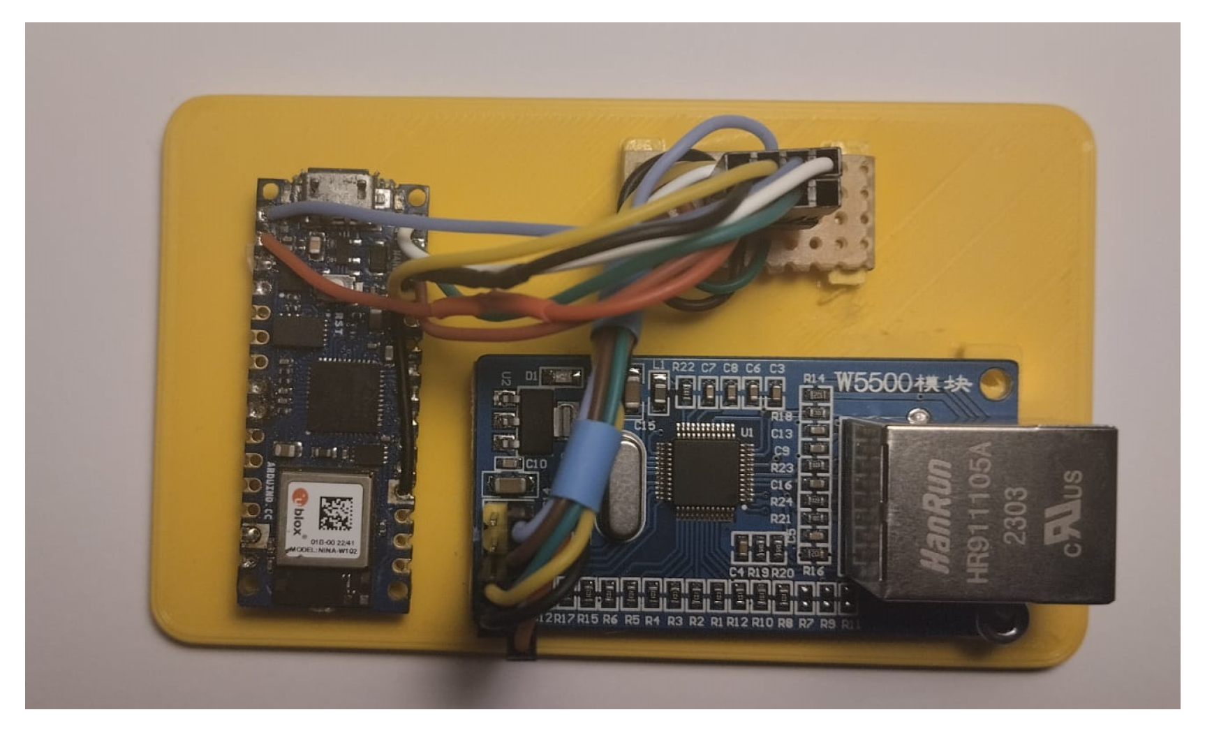
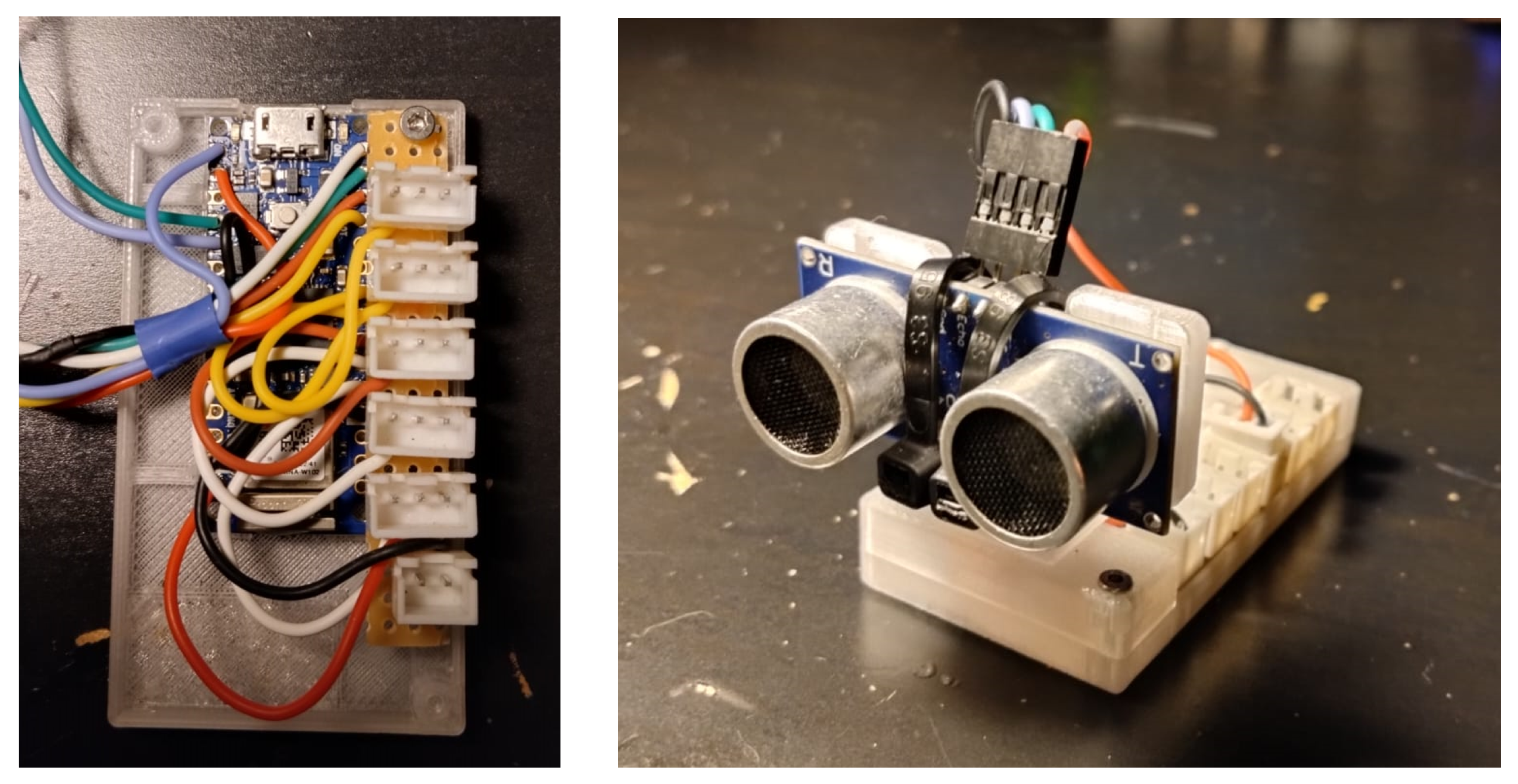
For the experimental scenario, the UDP communications were reformulated to work via Wi-Fi instead of Ethernet, which required minimal adjustment. A dedicated case was designed and 3D-printed to accommodate the Arduino board, the HC-SR04 ultrasonic sensor and a support PCB for the servo and ESC connectors, which can be seen in Figure 11.

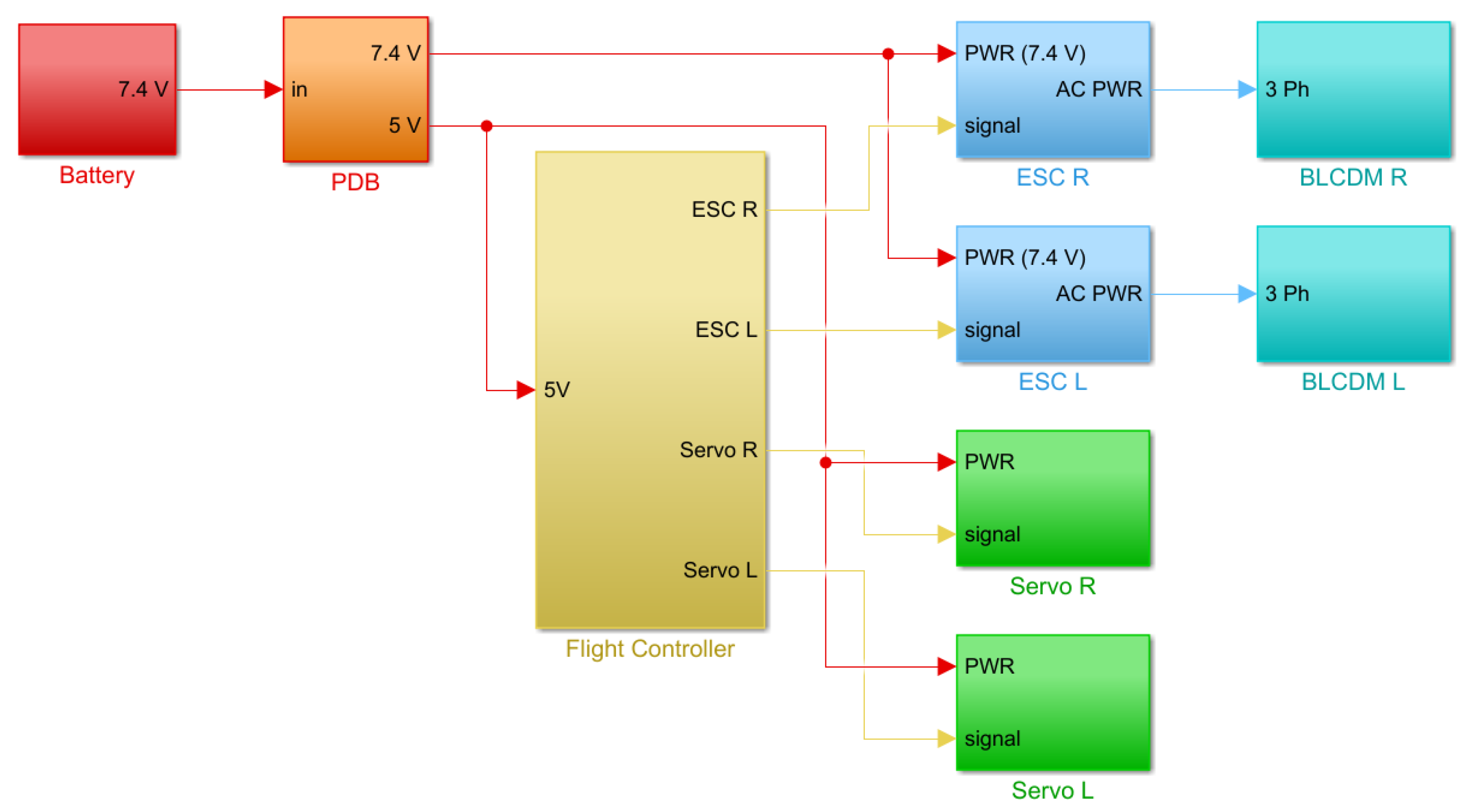
The integration of the aforementioned FC into the frame of the X-Vert required additional steps as well, namely, providing power to the required components. A power distribution board (PDB) was included to regulate the voltage provided by the battery powering the ESCs, servos and flight controller to their adequate levels. The electronic components used in the experimental assembly were the following:

• Servos: Spektrum A220 4g servos [48];
• ESC: SkyRC 20A Nano ESC with BLHeli firmware [49];
• BLDC motors: E-Flite BL280 2600 Kv Brushless Outrunner Motor [50];
• PDB: Matek Mini Power Hub [51];
• Battery: Gens Ace 450 mAh 7.4 V battery [52].

Figure 12 presents a diagram of the connections of the different electronic components, which were assembled in the frame of the X-Vert, as shown previously in Figure 2.

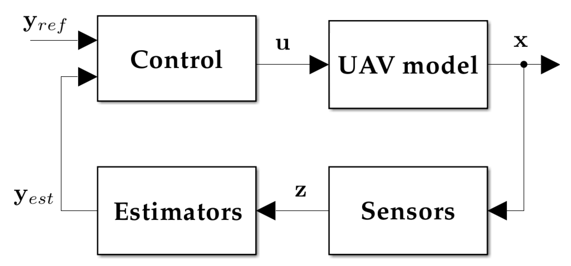
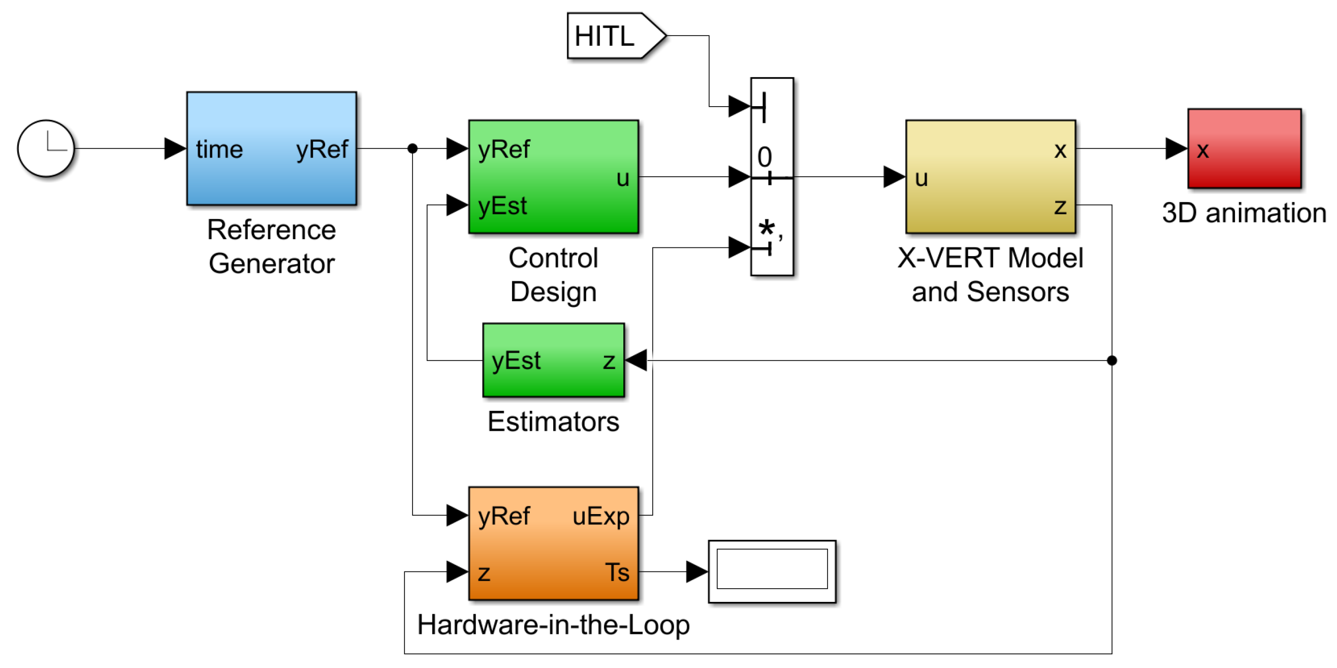
The management of the simulation was once again performed in Simulink, which was responsible for providing the references to the flight controller and for registering the control action and the estimated attitude computed by it.

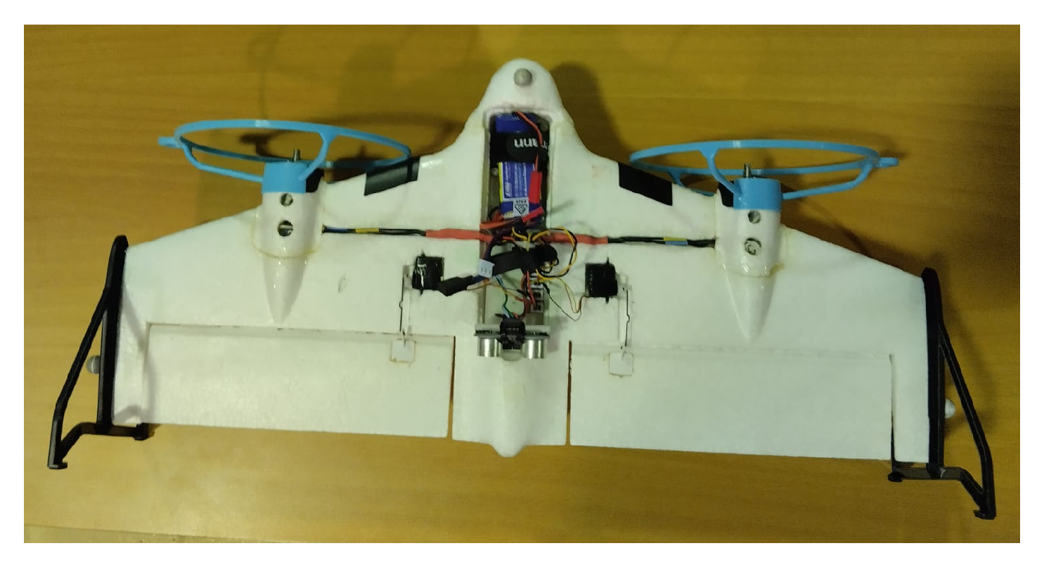
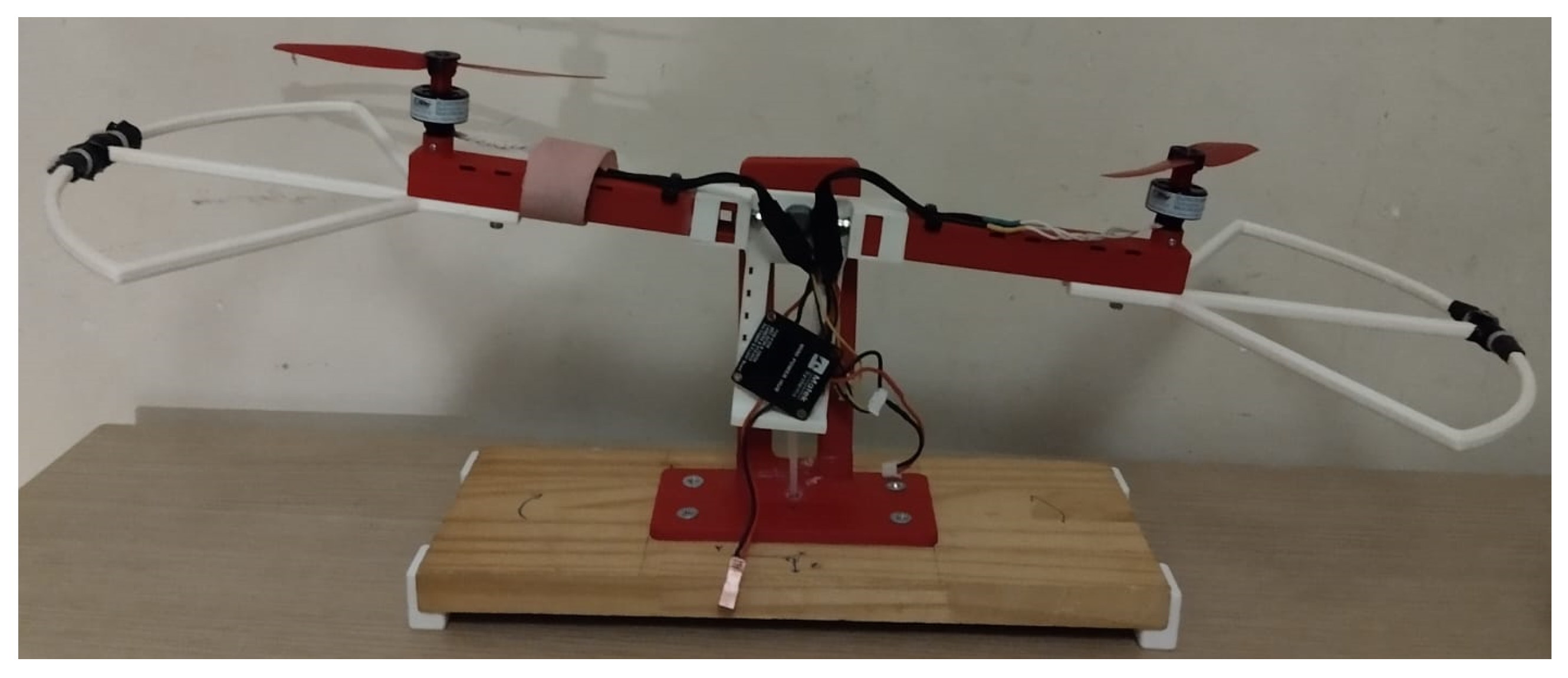
In order to verify the effectiveness of this communication strategy while also taking the opportunity to partially validate the different control strategies, a test assembly was designed and 3D-printed, comprising the electronics (with the exception of the servos) and propellers, as shown in Figure 13. Since the beam-like frame with the two motors and propellers is able to pivot around its center by means of a bearing, mounting the FC on it allows the testing of the stabilization algorithms on the z-axis of the UAV and also ensures that any errors and problems in the implementation are detected. This proved to be of vital importance since the X-Vert is a fragile aircraft, and initial crashes were demonstrated to significantly hinder development.

5.2. Ground Truth

In order to evaluate the performance of the controllers in the experimental scenario, a method for effectively tracking the position and attitude of the X-Vert is required. A motion capture system (MCS) covering an area of 12 by 4 m enveloped in a safety net, available at the host facility IDMEC—Instituto de Engenharia Mecânica—was used for this purpose. By using this set of cameras and the dedicated Qualysis Track Manager software by Qualysis [53], together with reflective markers placed on the surface of the X-Vert, it was possible to track both ${\mathbf{p}}^{NED}$ and ${\mathbf{q}}^{NED}$ with high precision inside the aforementioned area. Figure 14 shows the utilized installations and also provides an illustration of the area using the MCS, where the reconstruction of the X-Vert can be seen. The coordinate frame of the MCS does not match the previously described NED orientation, but care was taken to process the gathered data to account for the necessary conversion. Accounting for this, the position and orientation of the X-Vert provided by the MCS are assumed as the ground truth for the experimental trials and are therefore represented directly by ${\mathbf{p}}^{NED}$ and ${\mathbf{q}}^{NED}$, respectively.

5.3. Benchmark Maneuver for Experimental Vertical Flight

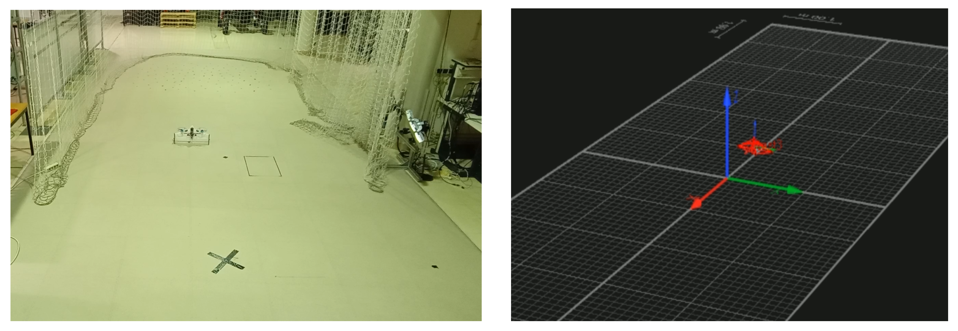
The benchmark maneuver described in Section 4 had to be adapted to the context of the experimental tests, where the available flight area is limited to the arena previously described. A decision was made to focus on the pitch control of the aircraft, as it was considered the most necessary to stabilize when in vertical flight and will present significant challenges for the transition to aerodynamic flight in future work. Therefore, the solution found for performing the experimental trials was to order the X-Vert to perform a take-off and hold its altitude at 0.5 m, manually guide it to the center of the arena if a substantial deviation happened during the initial maneuvers, and only then provide a set of references for $q_2$. 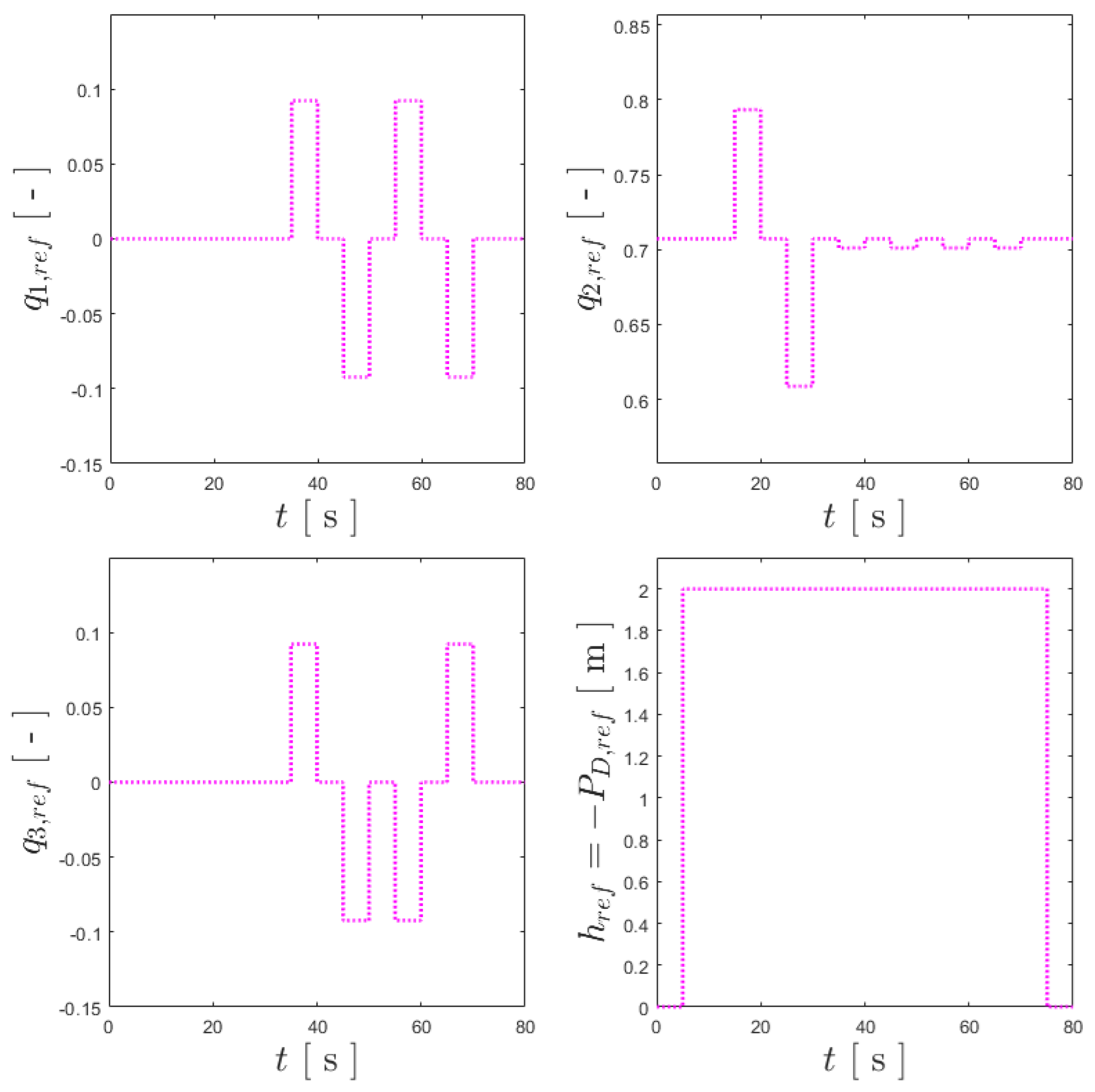This set consisted of rotating $-10$ degrees around the y-axis of the aircraft when it was fully vertical, holding this attitude for 2 s, returning to vertical orientation for 2 s, and then performing a symmetric rotation for another 2 s. This was carried out to ensure that the same reference would be provided during the tests for different controllers, allowing suitable conclusions to be drawn. Nonetheless, depending on the actual performance of the controller, additional lateral corrections were sometimes provided in order to prevent collisions, but this was avoided as much as possible.

An example of references of an experimental test, specifically the one performed for the BNC, is shown in Figure 15, which shows some small corrections during the process of guiding the UAV to the center of the arena, together with the aforementioned references of 2 s for $q_2$ and the constant reference altitude of 0.5 m.

5.4. Parameter Tuning for Experimental Flight

The adaptation to an experimental scenario necessitated another parameter tuning in order to accommodate such changes. It was soon realized that the Arduino Nano 33 IOT could not perform the cycles at 200 Hz when using UDP over Wi-Fi, and thus, a sample time $T_{s,exp}=0.01$ s was used instead, as it proved to be sufficiently low to stabilize the aircraft. The estimators and controllers were subject to a re-tuning as well, imposed not only by the transition from the simulation to the experimental setting but also by the change in the sampling frequency. Similarly to the simulation and HITL results, an effort was made to ensure that the parameters of the estimators and altitude controller were the same for the trials using different attitude controllers, and their values are

$${\alpha }_{CF}^{exp}=0.905,{\beta }_{CF}^{exp}=0.05,k_{p_D}^{exp}=10,k_u^{exp}=5$$

(64)

Regarding the controller gains and remaining parameters, these also had to be adjusted for the experimental trials, and the values are shown next:

• BNC (experimental): ${\mathbf{K}}_{ad}^{exp}=\mathrm{diag}[20,60,20]$, ${\mathbf{K}}_{ap}^{exp}=\mathrm{diag}[200,500,200]$;
• NDI (experimental): ${\mathbf{K}}_{\mathbf{w}}^{NDI,exp}=\mathrm{diag}[20,20,20]$, ${\mathbf{K}}_{\mathbf{q}}^{NDI,exp}=\mathrm{diag}[10,20,10]$;
• INDI (experimental): ${\mathbf{K}}_{\mathbf{w}}^{INDI,exp}=\mathrm{diag}[2,5,2]$, ${\mathbf{K}}_{\mathbf{q}}^{INDI,exp}=\mathrm{diag}[5,5,5]$, ${\omega }_{SD}^{sim}=100$, ${\tau }_{CF}^{exp}=0$, ${\lambda }^{exp}=0.2$.

As can be seen, ${\tau }_{CF}^{exp}=0$ implies the absence of the command filter described in Section 3. It was not deemed necessary since INDI already provided a smooth actuation, as will be described next, and the additional filtering introduced an unwanted delay.

5.5. Vertical Flight Results

Using the described setup, multiple trials were run for each of the controllers, and the data from each were registered using the following process: the references ${\mathbf{y}}_{ref}$, generated by MATLAB, were saved in a file generated at the end of each flight trial; in the same file, the quaternion ${\widehat{\mathbf{q}}}^{NED}$ estimated by the FC and the control action $\mathbf{u}$ computed by it and sent to MATLAB via Wi-Fi/UDP were also saved; and the orientation and position provided by the MCS, ${\mathbf{q}}^{NED}$ and ${\mathbf{p}}^{NED}$, 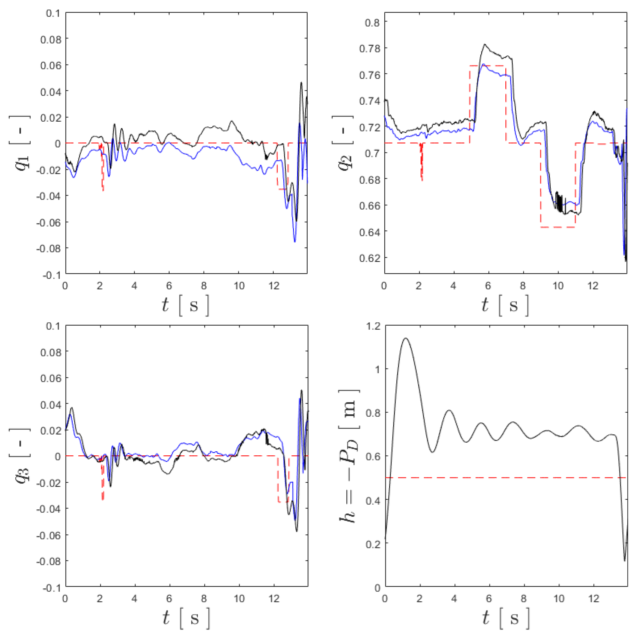were exported from the QTM software at the end of the trials to a separate file. Matching the timestamps of the two files, it was possible to overlap them, effectively allowing for the comparison of the reference quaternion, the respective estimation by the onboard FC and the quaternion provided by the MCS. Using the same experimental trial for the BNC, as shown in Figure 15, the curves for ${\mathbf{q}}_{ref}^{NED}$, ${\widehat{\mathbf{q}}}^{NED}$ and ${\mathbf{q}}^{NED}$—from take-off to landing—are shown in Figure 16, which also shows the comparison between the reference altitude $P_{D_{ref}}=-0.5$ [m] and its value provided by the MCS, assumed as the ground truth. It should be noted that the estimated altitude was considered to be of less relevance for the purpose of comparing attitude controllers and, thus, was omitted in order to reduce the amount of data being transmitted.

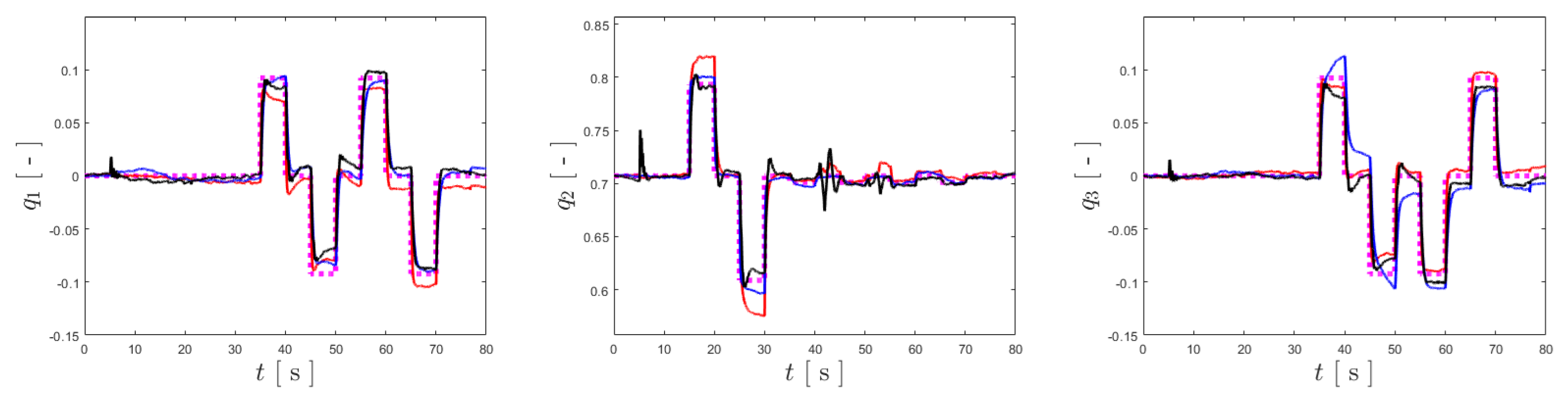
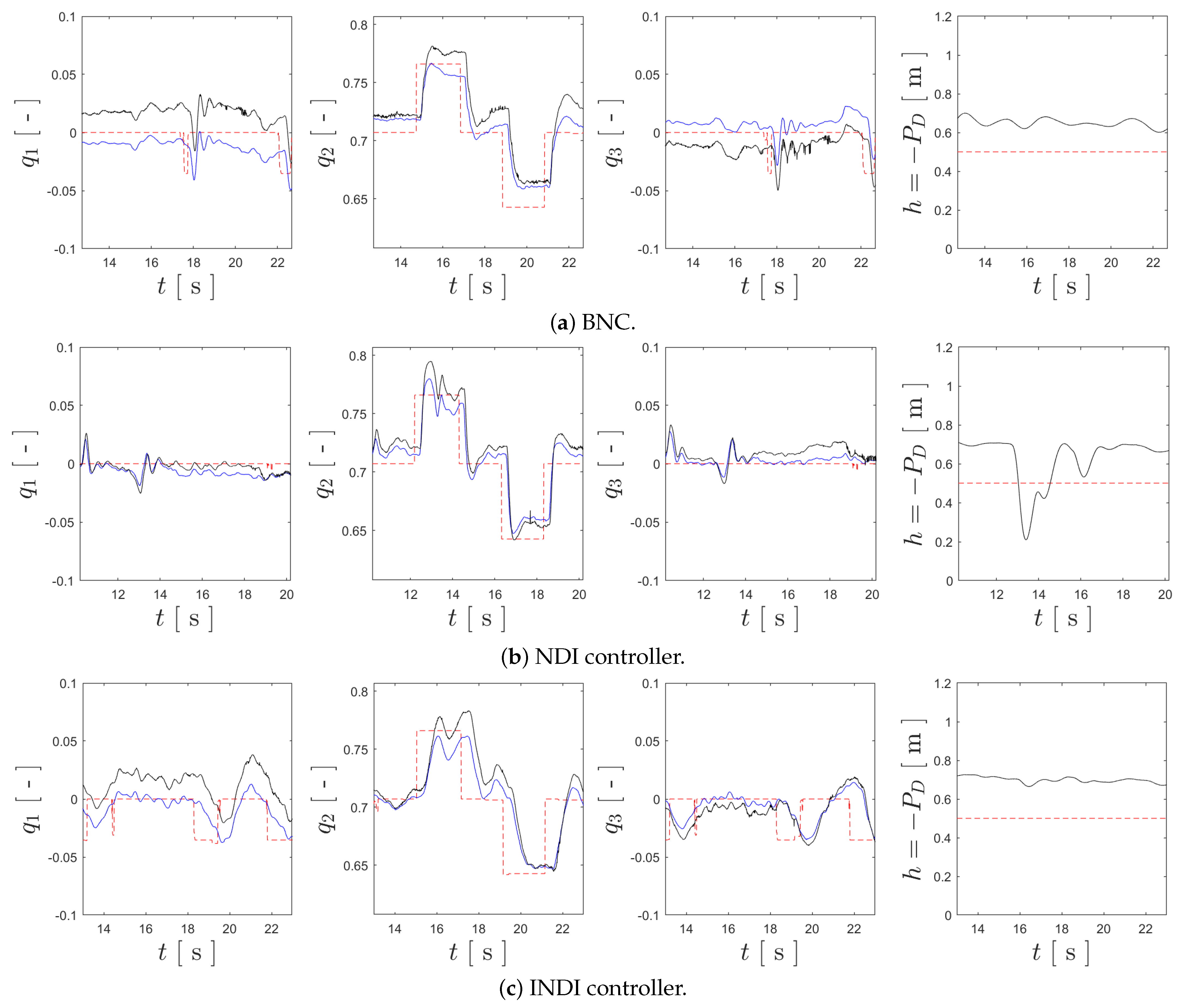
For the purposes of computing the evaluation metrics $RM{S}_q^{exp}$ and ${\mu }^{exp}$, a 10 s window was considered for each trial, corresponding to an interval of 2 s before and 2 s after the references were sent. This ensured that the comparison was fair, regardless of the length of the trials for each controller. Figure 17 presents the tracking results for each controller according this 10 s window of each flight trial.

Analyzing Figure 17, it is clear that all the controllers are capable of tracking the references in $q_2$ while also stabilizing the remaining degrees of freedom of the attitude. The BNC enables the accurate tracking of $q_2$, but its performance worsens for $q_1$ and $q_3$. On the other hand, the NDI controller manages to keep these closer to null values but has some some spikes when tracking $q_2$, although still managing to track it with precision. In the trial for the INDI controller strategy, additional lateral references were provided in order to avoid collisions, but the controller still managed to track the references. Nonetheless, since these lateral references were provided simultaneously to the $q_2$ references, some performance loss may have happened.

Table 3. Experimental results of tracking ${\mathbf{q}}_{ref}^{NED}$.

Cont.	${\mathit{RMS}}_{{\mathit{q}}_1}^{\mathit{exp}}$	${\mathit{RMS}}_{{\mathit{q}}_2}^{\mathit{exp}}$	${\mathit{RMS}}_{{\mathit{q}}_3}^{\mathit{exp}}$	${\overline{\mathit{RMS}}}_{\mathit{q}}^{\mathit{exp}}$
BNC	0.0219	0.0292	0.0149	0.0220
NDI	0.0071	0.0264	0.0115	0.0150
INDI	0.0271	0.0352	0.0232	0.0285

provides the evaluation metrics that summarize the tracking results for the experimental trials, where it can be seen that NDI has the best overall performance, while INDI has the worst, possibly evidencing the aforementioned loss of performance for this controller, and the BNC provides the middle ground among the three controllers. Lastly, regarding altitude tracking, it is clear that there was a sudden drop in altitude in the trial for the NDI controller, which was duly analyzed, and the explanation is provided after the analysis regarding actuator oscillation.

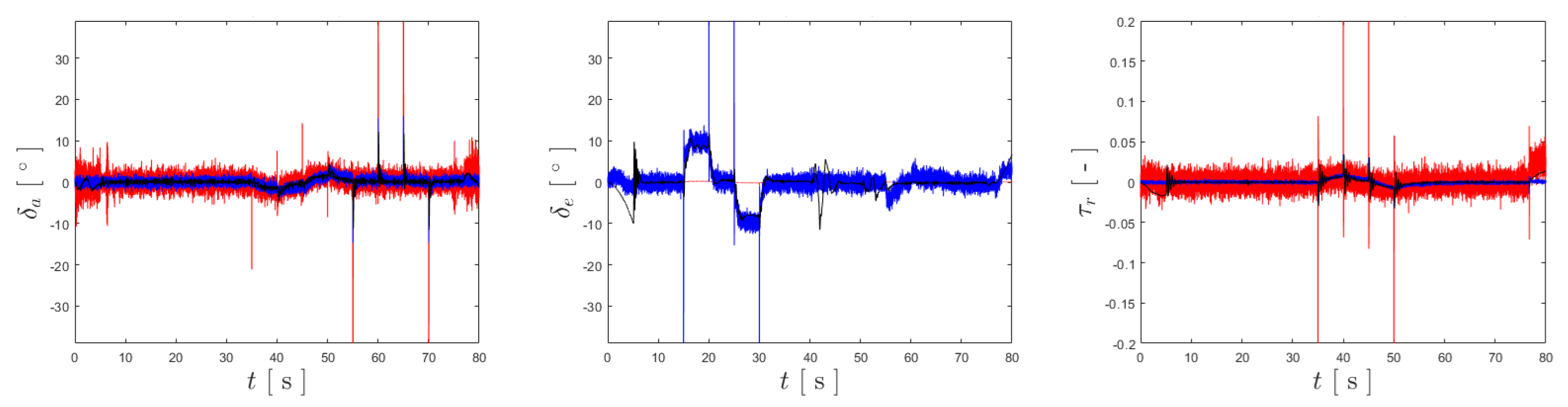
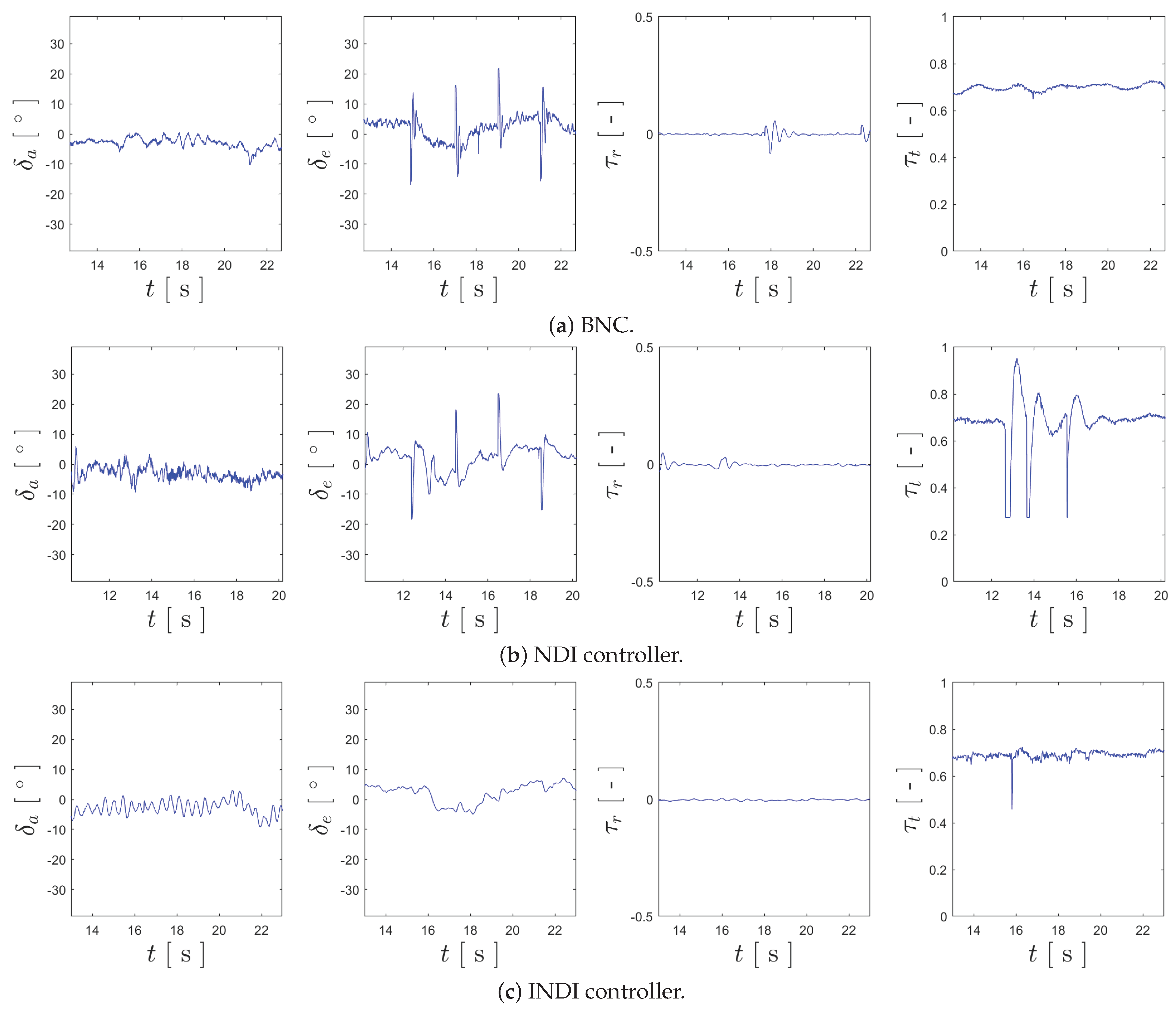
Moving on to the analysis of actuator oscillation, Figure 18 provides the plots of $\mathbf{u}={[{\delta }_a,{\delta }_e,{\tau }_r,{\tau }_t]}^T$ registered for the trial of each controller.

Focusing the analysis on the inputs used for attitude stabilization—${\delta }_a$, ${\delta }_e$ and ${\tau }_r$—the first obvious conclusion that can be drawn is that there is far less noise in the respective plots when compared to the simulation and HITL results. This may be explained by the reduction in the values of the gains but could also evidence excessive noise when modeling the sensors. Analyzing the smoothness of the curves in Figure 18, it can be stated that NDI and the BNC appear to be similar, with the BNC being more noisy for ${\delta }_a$ and NDI for ${\delta }_e$, and that there is virtually no oscillation for ${\tau }_r$ for all three controllers. For the elevator input, the INDI controller has a far smoother actuation when compared to the remaining two control strategies, not showing any of the sudden spikes that appear in the ${\delta }_e$ curves of the trials for NDI and the BNC. Nonetheless, the curve for ${\delta }_a$ has an almost constant oscillation, which could have been caused by the previously mentioned simultaneous lateral references during the maneuvers. Summarizing these results,

Table 4. Experimental results for oscillation of ${\mathit{u}}_{att}$.

Cont.	${\mathit{\mu }}_{{\mathit{\delta }}_{\mathit{a}}}^{\mathit{exp}}$	${\mathit{\mu }}_{{\mathit{\delta }}_{\mathit{e}}}^{\mathit{exp}}$	${\mathit{\mu }}_{{\mathit{\tau }}_{\mathit{r}}}^{\mathit{exp}}$	${\overline{\mathit{\mu }}}_{{\mathit{u}}_{\mathit{att}}}^{\mathit{exp}}$
BNC	0.0056	0.0213	0.0018	0.0095
NDI	0.0144	0.0156	0.0012	0.0104
INDI	0.0039	0.0018	0.0002	0.0020

provides the values for ${\mu }_{{\delta }_a}^{HITL}$, ${\mu }_{{\delta }_e}^{HITL}$ and ${\mu }_{{\tau }_r}^{HITL}$, as well as their average values.

Lastly, some considerations about the altitude control should be provided, namely, the sudden loss of altitude shown in Figure 17 for the experimental trial of the NDI controller. As Figure 18 also demonstrates for the same trial, the curve of ${\tau }_t$ has abrupt decreases, which cannot be explained by excessive altitude. A similar event also happened during the experimental flight with the INDI controller, although to a smaller degree. After thorough analysis, it was found that this was caused by the partial obstruction of the sonar by the tail of the X-Vert when its pitch went beyond 90 degrees. Since this obstruction caused the sonar not to receive a response signal (activating a timeout), it assumed a far greater altitude than the real one, and the controller responded accordingly, decreasing the throttle input. This issue was acknowledged, and in general, the controllers demonstrated robustness to its influence, but it should be addressed in future work.

In summary, the general conclusions for the experimental flight tests largely agree with those drawn for the simulation and HITL scenarios when comparing the values of ${\overline{RMS}}_q$ and ${\overline{\mu }}_{u_{att}}$ for each. Some discrepancies are found when comparing the performance of each controller among the three scenarios, which can happen due to possible mismatches between the X-Vert simulation model and the real aircraft, the robustness of each control method to such discrepancies, and the tuning parameters of each controller, such as the gains, among others. These discrepancies are therefore expected to arise, but the conclusions drawn are qualitatively the same, as they confirm that all the control solutions are capable of tracking the references, with the INDI controller standing out by providing a smoother control action with less actuator oscillation.

6. Conclusions

In this research work, a simulator for a tail-sitter UAV was developed, allowing for the testing of different control strategies in a simulated scenario. The attitude controllers tested were of a nonlinear nature, with one being from a previous work developed for the same aircraft [29], one being based on Nonlinear Dynamic Inversion principles, and the last being its incremental version, INDI. The controllers and estimators were implemented in an Arduino board and integrated into the simulated environment in order to enable Hardware-in-the-Loop testing of the control solutions. The simulation and HITL results for performing standard maneuvers in vertical flight demonstrated that all the implemented controllers manage to track the references, although the INDI control strategy stands out by providing a far smoother actuation. Advancing to an experimental scenario, a tail-sitter was adapted in order to accept the Arduino-based flight controller, and indoor experimental trials for vertical flight were conducted. The results of these highlight once again the smoothness of actuation of the INDI control strategy, nonetheless demonstrating that all the implemented controllers are capable of stabilizing the X-Vert in vertical flight and tracking the provided references.

As an overview of the achievements of this work, a major contribution of this work is the streamlined development and testing of different control solutions: these are first developed in simulations, then validated with the HITL tools using the same simulated model after the implementation of the control solution for the flight controller, and finally tested with an experimental setup. This integrated pipeline facilitates the iterative and structured development and test of flight control solutions, which proved to be crucial for this research work, as they allowed the three controllers to be implemented and evaluated using the same metrics. The fact that the different control solutions were able to stabilize the X-Vert in vertical flight provides another considerable contribution, where INDI demonstrated increased robustness to sensor noise, evidenced by a smoother control action, which is beneficial and less demanding for the physical actuators of the aircraft. An obvious limitation of this work to be noted is the negative effect of sonar on altitude control, which, despite appearing to not have had a noteworthy impact on the attitude tracking results, is obviously unwanted. In future iterations of this research, is it advised to complement the altitude estimation with a barometer and to use sonar only for specific take-off and landing moments, and not during maneuvers for significant attitude changes.

Continuing on the topic of future work, the suggested continuation is to explore the performance of the BNC, NDI and INDI control solutions for an outdoor scenario, where aerodynamic flight can be performed. This will require a new iteration of the flight controller, accounting for new sensors to estimate the necessary variables—such as airspeed—and may necessitate the reformulation of the estimation methods to account for these. Additionally, this introduces the challenge of transitioning to and from aerodynamic flight, and the control strategies have to be robust enough to enable a safe transition, which will eventually also require reformulation to account for non-zero airspeed. Nonetheless, a robust vertical flight is crucial for tail-sitters to ensure safe take-off and landing maneuvers, and therefore, this research provides major contributions on this topic and is expected to progress to the aforementioned aspects in future iterations.

References

1. Telli, K.; Kraa, O.; Himeur, Y.; Ouamane, A.; Boumehraz, M.; Atalla, S.; Mansoor, W. A comprehensive review of recent research trends on unmanned aerial vehicles (uavs). Systems 2023, 11, 400. [Google Scholar] [CrossRef]
2. Xu, H.; Wang, L.; Han, W.; Yang, Y.; Li, J.; Lu, Y.; Li, J. A Survey on UAV Applications in Smart City Management: Challenges, Advances, and Opportunities. IEEE J. Sel. Top. Appl. Earth Obs. Remote Sens. 2023, 16, 8982–9010. [Google Scholar] [CrossRef]
3. Chehreh, B.; Moutinho, A.; Viegas, C. Latest Trends on Tree Classification and Segmentation Using UAV Data—A Review of Agroforestry Applications. Remote Sens. 2023, 15, 2263. [Google Scholar] [CrossRef]
4. Rakesh, D.; Kumar, N.A.; Sivaguru, M.; Keerthivaasan, K.V.R.; Janaki, B.R.; Raffik, R. Role of UAVs in innovating agriculture with future applications: A review. In Proceedings of the 2021 International Conference on Advancements in Electrical, Electronics, Communication, Computing and Automation (ICAECA), Coimbatore, India, 8–9 October 2021. [Google Scholar]
5. Saeed, A.S.; Younes, A.B.; Cai, C.; Cai, G. A survey of hybrid unmanned aerial vehicles. Prog. Aerosp. Sci. 2018, 98, 91–105. [Google Scholar] [CrossRef]
6. Ducard, G.J.; Allenspach, M. Review of designs and flight control techniques of hybrid and convertible VTOL UAVs. Aerosp. Sci. Technol. 2021, 118, 107035. [Google Scholar] [CrossRef]
7. Misra, A.; Jayachdran, S.; Kenche, S.; Katoch, A.; Suresh, A.; Gundabattini, E.; Selvaraj, S.K.; Legesse, A.A. A Review on Vertical Take-Off and Landing (VTOL) Tilt-Rotor and Tilt Wing Unmanned Aerial Vehicles (UAVs). J. Eng. 2022, 2022, 1803638. [Google Scholar] [CrossRef]
8. Okasha, M.; Shah, J.; Fauzi, W.; Hanouf, Z. Gain scheduled linear quadratic control for quadcopter. IOP Conf. Ser. Mater. Sci. Eng. 2017, 270, 012009. [Google Scholar] [CrossRef]
9. Poksawat, P.; Wang, L.; Mohamed, A. Gain scheduled attitude control of fixed-wing UAV with automatic controller tuning. IEEE Trans. Control. Syst. Technol. 2017, 26, 1192–1203. [Google Scholar] [CrossRef]
10. Qiao, J.; Liu, Z.; Zhang, Y. Gain scheduling based PID control approaches for path tracking and fault tolerant control of a quad-rotor UAV. Int. J. Mech. Eng. Robot. Res. 2018, 7, 401–408. [Google Scholar] [CrossRef]
11. Melo, A.G.; Andrade, F.A.; Guedes, I.P.; Carvalho, G.F.; Zachi, A.R.; Pinto, M.F. Fuzzy gain-scheduling PID for UAV position and altitude controllers. Sensors 2022, 22, 2173. [Google Scholar] [CrossRef]
12. Pashilkar, A.A.; Ismail, S.; Ayyagari, R.; Sundararajan, N. Design of a nonlinear dynamic inversion controller for trajectory following and maneuvering for fixed wing aircraft. In Proceedings of the 2013 IEEE Symposium on Computational Intelligence for Security and Defense Applications (CISDA), Singapore, 16–19 April 2013. [Google Scholar]
13. Azinheira, J.R.; Moutinho, A. Hover Control of an UAV with Backstepping Design Including Input Saturations. IEEE Trans. Control. Syst. Technol. 2014, 16, 517–526. [Google Scholar] [CrossRef]
14. Horn, J.F. Non-linear dynamic inversion control design for rotorcraft. Aerospace 2019, 6, 38. [Google Scholar] [CrossRef]
15. Wang, F.; Wang, P.; Deng, H.; Chen, B. Nonlinear Dynamic Inversion Control of VTOL Tilt-Wing UAV. In Proceedings of the 2018 Eighth International Conference on Instrumentation & Measurement, Computer, Communication and Control (IMCCC), Harbin, China, 19–21 July 2018. [Google Scholar]
16. Fu, Y.; Zhang, Y.; Yu, Z.; Liu, Z. A Backstepping Control Strategy for Fixed Wing UAV under Actuator Failure. In Proceedings of the 2019 IEEE 28th International Symposium on Industrial Electronics (ISIE), Vancouver, BC, Canada, 12–14 June 2019. [Google Scholar]
17. Smeur, E.J.; Chu, Q.; De Croon, G.C. Adaptive incremental nonlinear dynamic inversion for attitude control of micro air vehicles. J. Guid. Control. Dyn. 2016, 39, 450–461. [Google Scholar]
18. Azinheira, J.R.; Moutinho, A.; Carvalho, J.R. Lateral control of airship with uncertain dynamics using incremental nonlinear dynamics inversion. IFAC Pap. Online 2015, 48, 69–74. [Google Scholar] [CrossRef]
19. Sieberling, S.; Chu, Q.P.; Mulder, J.A. Robust flight control using incremental nonlinear dynamic inversion and angular acceleration prediction. J. Guid. Control. Dyn. 2019, 33, 1732–1742. [Google Scholar] [CrossRef]
20. Acquatella, P.; van Kampen, E.; Chu, Q.P. Incremental backstepping for robust nonlinear flight control. In Proceedings of the EuroGNC 2013, Delft, The Netherlands, 10–12 April 2013. [Google Scholar]
21. Guerreiro, N.M.; Moutinho, A. Robust incremental backstepping controller for the attitude and airspeed tracking of a commercial airplane. In Proceedings of the 2019 IEEE 10th International Conference on Mechanical and Aerospace Engineering (ICMAE), Brussels, Belgium, 22–25 July 2019. [Google Scholar]
22. Cordeiro, R.A.; Azinheira, J.R.; Moutinho, A. Robustness of incremental backstepping flight controllers: The boeing 747 case study. IEEE Trans. Aerosp. Electron. Syst. 2021, 57, 3492–3505. [Google Scholar] [CrossRef]
23. Tal, E.; Karaman, S. Accurate tracking of aggressive quadrotor trajectories using incremental nonlinear dynamic inversion and differential flatness. IEEE Trans. Control. Syst. Technol. 2020, 29, 1203–1218. [Google Scholar] [CrossRef]
24. Jayaraman, B.; Giri, D.K.; Ghosh, A.K. Attitude Tracking Control of a Light Aircraft Using Classical and Incremental Nonlinear Dynamic Inversion Approaches. In Proceedings of the 2021 International Conference on Unmanned Aircraft Systems (ICUAS), Athens, Greece, 15–18 June 2021. [Google Scholar]
25. Smeur, E.J.; Bronz, M.; de Croon, G.C. Incremental control and guidance of hybrid aircraft applied to a tailsitter unmanned air vehicle. J. Guid. Control. Dyn. 2020, 43, 274–287. [Google Scholar] [CrossRef]
26. Tal, E.A.; Karaman, S. Global trajectory-tracking control for a tailsitter flying wing in agile uncoordinated flight. In Proceedings of the AIAA Aviation 2021 Forum, Online, 2–6 August 2021. [Google Scholar]
27. Tal, E.; Karaman, S. Global incremental flight control for agile maneuvering of a tailsitter flying wing. J. Guid. Control. Dyn. 2022, 45, 2332–2349. [Google Scholar] [CrossRef]
28. Yang, Y.; Zhu, J.; Yang, J. INDI-based transitional flight control and stability analysis of a tail-sitter UAV. In Proceedings of the 2020 IEEE International Conference on Systems, Man, and Cybernetics (SMC), Toronto, ON, Canada, 11–14 October 2020. [Google Scholar]
29. Chiappinelli, R.; Nahon, M. Modeling and Control of a Tailsitter UAV. In Proceedings of the 2018 International Conference on Unmanned Aircraft Systems (ICUAS), Dallas, TX, USA, 12–15 June 2018. [Google Scholar]
30. E-Flite XVERT VTOL Webpage. Available online: https://www.horizonhobby.de/en_DE/product/x-vert-vtol-bnf-basic-504mm/EFL1850.html (accessed on 24 January 2024).
31. Beard, R.W.; McLain, T.W. Small Unmanned Aircraft: Theory and Practice, 1st ed.; Princeton University Press: Princeton, NJ, USA, 2018. [Google Scholar]
32. Stevens, B.L.; Lewis, F.L. Aircraft Control and Simulation: Dynamics, Controls Design, and Autonomous Systems, 3rd ed.; John Wiley & Sons: Hoboken, NJ, USA, 2016. [Google Scholar]
33. Nelson, R.C. Flight Stability and Automatic Control, 2nd ed.; McGraw-Hill: New York, NY, USA, 1998. [Google Scholar]
34. Whidborne, J.; Mendez, A.; Cooke, A. Effect of Rotor Tilt on the Gust Rejection Properties of Multirotor Aircraft. Drones 2022, 6, 305. [Google Scholar] [CrossRef]
35. Khan, W.; Nahon, M. Toward an accurate physics-based UAV thruster model. IEEE ASME Trans. Mechatron. 2013, 18, 1269–1279. [Google Scholar] [CrossRef]
36. McCormick, B.W. Aerodynamics, Aeronautics and Flight Mechanics, 2nd ed.; John Wiley & Sons: Hoboken, NJ, USA, 1979. [Google Scholar]
37. Khan, W.; Nahon, M. Real-time modeling of agile fixed-wing UAV aerodynamics. In Proceedings of the 2015 International Conference on Unmanned Aircraft Systems (ICUAS), Denver, CO, USA, 9–12 June 2015. [Google Scholar]
38. Khan, W.; Nahon, M. Modeling dynamics of agile fixed-wing UAVs for real-time applications. In Proceedings of the 2016 International Conference on Unmanned Aircraft Systems (ICUAS), Arlington, VA, USA, 7–10 June 2016. [Google Scholar]
39. Prisacariu, V.; Cîrciu, I.; Boscoianu, M. Flying wing aerodynamic analysis. Rev. Air Force Acad. 2012, 2, 31–35. [Google Scholar]
40. Esteves, D.J.; Moutinho, A.; Azinheira, J.R. Stabilization and altitude control of an indoor low-cost quadrotor: Design and experimental results. In Proceedings of the 2015 IEEE International Conference on Autonomous Robot Systems and Competitions, Vila Real, Portugal, 8–10 April 2015. [Google Scholar]
41. Madgwick, S.O.; Harrison, A.J.; Vaidyanathan, R. Estimation of IMU and MARG orientation using a gradient descent algorithm. In Proceedings of the 2011 IEEE International Conference on Rehabilitation Robotics, Zurich, Switzerland, 29 June–1 July 2011. [Google Scholar]
42. Acquatella, P.; van Ekeren, W.; Chu, Q.P. Pi (d) tuning for flight control systems via incremental nonlinear dynamic inversion. IFAC Pap. Online 2017, 50, 8175–8180. [Google Scholar] [CrossRef]
43. Cordeiro, R.A.; Azinheira, J.R.; Moutinho, A. Cascaded incremental backstepping controller for the attitude tracking of fixed-wing aircraft. In Proceedings of the 5th CEAS Conference on Guidance, Navigation and Control, Berlin, Germany, 3–5 April 2019. [Google Scholar]
44. Cordeiro, R.A.; Marton, A.S.; Azinheira, J.R.; Carvalho, J.R.; Moutinho, A. Increased robustness to delay in incremental controllers using input scaling gain. IEEE Trans. Aerosp. Electron. Syst. 2021, 58, 1199–1210. [Google Scholar] [CrossRef]
45. Arduino Nano 33 IOT Product Page. Available online: https://docs.arduino.cc/hardware/nano-33-iot/ (accessed on 24 January 2024).
46. Wiznet W5500 Product Page. Available online: https://www.wiznet.io/product-item/w5500/ (accessed on 24 January 2024).
47. CAD Model UAV Tailsitter at GrabCAD Website. Available online: https://grabcad.com/library/uav-tailsitter-1 (accessed on 24 January 2024).
48. Spektrum A220 4g Aircraft Servo Product Page, Horizon Hobby Website. Available online: https://www.horizonhobby.com/product/a220-4g-aircraft-servo-x-vert/SPMSA220.html (accessed on 24 January 2024).
49. 20A Nano ESC Product Page, SkyRC Website. Available online: https://www.skyrc.com/Discontinued_Products/20A_ESC (accessed on 24 January 2024).
50. BL280 Brushless Outrunner Motor 2600Kv Product Page, Horizon Hobby Website. Available online: https://www.horizonhobby.com/product/bl280-brushless-outrunner-motor-2600kv/EFLM1809.html (accessed on 24 January 2024).
51. Mini Power Hub Product Page, MatekSys Website. Available online: http://www.mateksys.com/?portfolio=hub5v12v#tab-id-1 (accessed on 24 January 2024).
52. Gens Ace G-Tech Soaring 450 mAh 7.4 V Battery Product Page, Gens Ace Website. Available online: https://www.gensace.de/gens-ace-g-tech-soaring-450mah-7-4v-30c-2s1p-lipo-battery-pack-with-jst-syp-plug.html (accessed on 24 January 2024).
53. Qualysis Track Manager Software, Qualysis Website. Available online: https://www.qualisys.com/software/qualisys-track-manager/ (accessed on 24 January 2024).
Figure 1. Simulation environment.
Robotics 13 00051 g001
Figure 2. The experimental prototype based on the frame of the X-Vert VTOL.
Robotics 13 00051 g002
Figure 3. The division of the wing into three zones for the computation of the aerodynamic forces and moments according to different angle-of-attack and airspeed values, as well as elevon deflection.
Robotics 13 00051 g003
Figure 4. A block diagram representing the implementation of the INDI controller: the angular acceleration w ˙ g B is estimated from w g , g y r B using (58) and then compared to the desired dynamics w ˙ g , d B , and the difference is used to compute the required control increment. This is added to the control action of the previous time-step, being filtered by (59) and subject to actuator saturation.
Robotics 13 00051 g004
Figure 5. The assembly designed for HITL development comprising the Arduino Nano 33 IOT board on the left, the W5500 Ethernet adapter on the bottom right and the adapter PCB on the top right.
Robotics 13 00051 g005
Figure 6. References for the benchmark maneuver for vertical flight: in the upper-left corner, q 1 , r e f ; in the upper-right corner, q 2 , r e f ; in the lower-left corner, q 3 , r e f ; and in the lower-right corner, P D , r e f .
Robotics 13 00051 g006
Figure 7. An overview of the Simulink environment developed for testing the attitude control solutions.
Robotics 13 00051 g007
Figure 8. The Simulink 3D environment with a tail-sitter model [47].
Robotics 13 00051 g008
Figure 9. Tracking results for q 1 , q 2 and q 3 , ordered from left to right. The references are shown by the pink dashed lines, and the results for the BNC, NDI and INDI are represented in red, blue and black.
Robotics 13 00051 g009
Figure 10. Plots for δ a , δ e and τ r , ordered from left to right. The inputs generated by the BNC are represented in red, the ones from NDI are shown in blue, and INDI is in black.
Robotics 13 00051 g010
Figure 11. The flight controller based on the Arduino Nano 33 IOT with the servo and ESC connectors (left) and the full assembly of the FC with the HC-SR04 ultrasonic sensor (right).
Robotics 13 00051 g011
Figure 12. A diagram of the electronics of the experimental assembly. From left to right: battery (red); PDB (orange); FC (yellow); ESCs (blue); BLDC motors (cyan); and servos (green). The power supply lines can be seen in red displaying the respective voltage levels, the signal lines provided by the FC are shown in yellow, and the three-phase ones are shown in blue.
Robotics 13 00051 g012
Figure 13. The 3D-printed test assembly designed to validate the communications and controller implementation, showing the proprotors, ESCs and PDB.
Robotics 13 00051 g013
Figure 14. On the left: the 12-by-4 m net-protected arena used. On the right: a 3D reconstruction of the X-Vert using the MCS.
Robotics 13 00051 g014
Figure 15. References for the experimental trial for the BNC.
Robotics 13 00051 g015
Figure 16. The full-length experimental trial for the BNC, where the references are shown by the red dashed line, the ground truth is represented by black, and the estimated values are presented in blue.
Robotics 13 00051 g016
Figure 17. Tracking results for the different attitude controllers, where the references are shown by the red dashed line, the ground truth is represented by black, and the estimated values are presented in blue.
Robotics 13 00051 g017
Figure 18. Plots of each component of u = [ δ a , δ e , τ r , τ t ] T recorded during the flight trials of each controller.
Robotics 13 00051 g018