Abstract
Due to space and energy restrictions, lightweight autonomous underwater vehicles (AUVs) are usually fitted with low-power processing units, which limits the ability to run demanding applications in real time during the mission. However, several robotic perception tasks reveal a parallel nature, where the same processing routine is applied for multiple independent inputs. In such cases, leveraging parallel execution by offloading tasks to a GPU can greatly enhance processing speed. This article presents a collection of generic matrix manipulation kernels, which can be combined to develop parallelized perception applications. Taking advantage of those building blocks, we report a parallel implementation for the 3DupIC algorithm—a probabilistic scan matching method for sonar scan registration. Tests demonstrate the algorithm’s real-time performance, enabling 3D sonar scan matching to be executed in real time onboard the EVA AUV.
Keywords:
underwater; sonar; scan matching; Coda Octopus Echoscope; 3DupIC; mapping; localization; AUV; OpenCL; GPU; real time 1. Introduction
In recent times, there has been a growing demand for autonomous underwater vehicles (AUVs) to perform various applications, such as offshore structure inspection, exploration of underwater environments, environmental and habitat monitoring, and more. Recent statistics show an increasing interest in research areas related to the development of underwater robots, with particular relevance in topics of localization and navigation [1].
Robotic localization concerns about determining an updated solution for the robot’s current pose within a well-defined global reference frame. It is commonly accepted that robust, accurate and long-term localization cannot be achieved through a single sensor [2]. Therefore, modern methods for robotic localization rely on data fusion techniques to combine measurements from complementary sensors in an effort to compensate for the weaknesses of each device [3] and achieve robust long-term performance.
The problem is usually found in addressed using probabilistic state estimation methods, implementing a dead reckoning core, associated with a high rate sensor to preform prediction. In underwater applications, inertial motion unit (IMU) and Doppler Velocity Log (DVL) constitute two valuable devices for performing dead reckoning. IMUs provide high rate linear accelerations and angular velocity measurements, which, through integration, produce position and attitude estimates. On the other hand, DVLs directly measure linear velocities of the robot with respect to the seafloor.
Since dead reckoning is susceptible to drift, state corrections from other sensors, preferably producing direct state observations, are necessary to ensure long-term consistency. Unfortunately, the acquisition of global localization fixes is not straightforward underwater.
The use of the Global Navigation Satellite System (GNSS) is possible on the surface to retrieve accurate position and heading corrections [4]. However, due to the attenuation of electromagnetic waves underwater, this resource becomes unavailable as soon as the vehicle dives. Acoustic positioning solutions [5] enable the computation of relative position between nodes equipped with compatible transponders. Nevertheless, since this solution requires the installation of an external infrastructure, it is not practical for most applications.
Another possibility, explored in this article, relies on sensing the surrounding environment to retrieve robot displacement estimates. In underwater environments, ranging sonars constitute a robust source of geometric data, from which displacement measurements can be extracted using scan matching techniques. Given two range scans of the same static scene, taken from different perspectives, the scan matching process computes the rigid body transformation that brings the scans together in the same reference frame. Assuming the sensor is fixed with respect to the robot frame, the transformation that best overlaps the two scans corresponds to the relative robot displacement between scan acquisition poses. Displacements computed through scan matching can be integrated into the localization system in two ways: either inserted in the dead reckoning core, as highly accurate odometry references, or they can be integrated in a SLAM system to provide relative displacements and loop closure constraints.
By its simplicity, the iterative closest point (ICP) is a popular scan matching technique [6]. It recursively minimizes the distance between point-to-point matches, selected using the Euclidean distance. Countless variants of the ICP algorithm have been proposed [7,8], either to increase speed [9] or improve robustness, convergence and accuracy [7,8,10,11,12]. Most registration methods were originally developed for terrestrial applications, assuming that high resolution and accurate range measurements are readily available from Light Detection and Ranging (LIDAR) sensors. In underwater environments, current sonar ranging technology offers significantly lower resolution, reduced sampling rates and higher percentage of outliers. As a result, scan matching methods tailored to these specific conditions are required.
Probabilistic scan matching formulations incorporate not only range measurements but also account for their uncertainty. This becomes particularly relevant when measurement uncertainty is high, as is the case of underwater sonars [13]. Building upon the initial pIC method [14], several variants were introduced to target the unique characteristics of each sonar type, with reported applications for imaging [15,16] and profiling sonars [13,17,18]. All these techniques involve an intermediate sub-map building stage, which is used to form dense patches of the scene, that can be later registered through scan matching. The submap building stage requires short-term accurate dead reckoning, which can be a limitation in underwater scenarios, where DVL dropouts and measurement outliers may negatively affect the localization accuracy.
In the past, we have presented a probabilistic scan matching technique specifically developed for registration of 3D scans from an Echoscope acoustic camera—the 3D underwater probabilistic iterative correspondence (3DupIC) [19]. It differs from previous techniques as it eliminates the need for submap construction, enabling its application in situations of degraded dead reckoning. On the downside, the algorithm involves complex matrix calculations that, when executed sequentially on the AUV’s processor, lead to computational overload with wait times far exceeding the desired real-time response. As described in the next section, the 3DupIC is an iterative algorithm that repeats two main tasks until convergence: (1) establish point to point matches; (2) minimize the Mahalanobis distance between compatible point pairs. In both stages, either individual points and point pairs are assumed to be independent, making the processing operations well suited for parallelization.
The key contribution of this article is the report of a GPU-accelerated implementation of the 3DupIC algorithm, capable of achieving real-time responses. With a divide-and-conquer philosophy, the problem was broken down into a set of basic matrix operations, for which the code is provided in this article. These building blocks can be reused to achieve accelerated implementations of other computationally intensive tasks involving large matrices. Furthermore, the adoption of Open Computing Language (OpenCL) [20], a platform agnostic framework for parallel programming, facilitates integration in other systems with hardware from different vendors. Performance tests on an embedded computer demonstrate the ability to run the algorithm in real time, enabling its use in a fully operational AUV.
This article is organized as follows. Section 2 presents the 3DupIC method, describing the probabilistic model applied to each sonar beam, the point matching strategy and the error minimization procedure. Section 3 explores the OpenCL programming concepts and details the developed processing kernels. Section 4 describes how the kernels from Section 3 are combined and launched to execute the 3DupIC algorithm from Section 2. Experimental tests demonstrating the real-time capabilities are presented in Section 5. Finally, Section 6 provides the conclusion.
2. 3DupIC Scan Matching
The 3DupIC [19] is a probabilistic scan matching method, which adapts the original probabilistic iterative correspondence (pIC) [14] to perform registration, in six degrees of freedom, of 3D scans acquired from an Echoscope 3D underwater sonar. The probabilistic formulation allows noise to be considered during the point matching and error optimization stages.
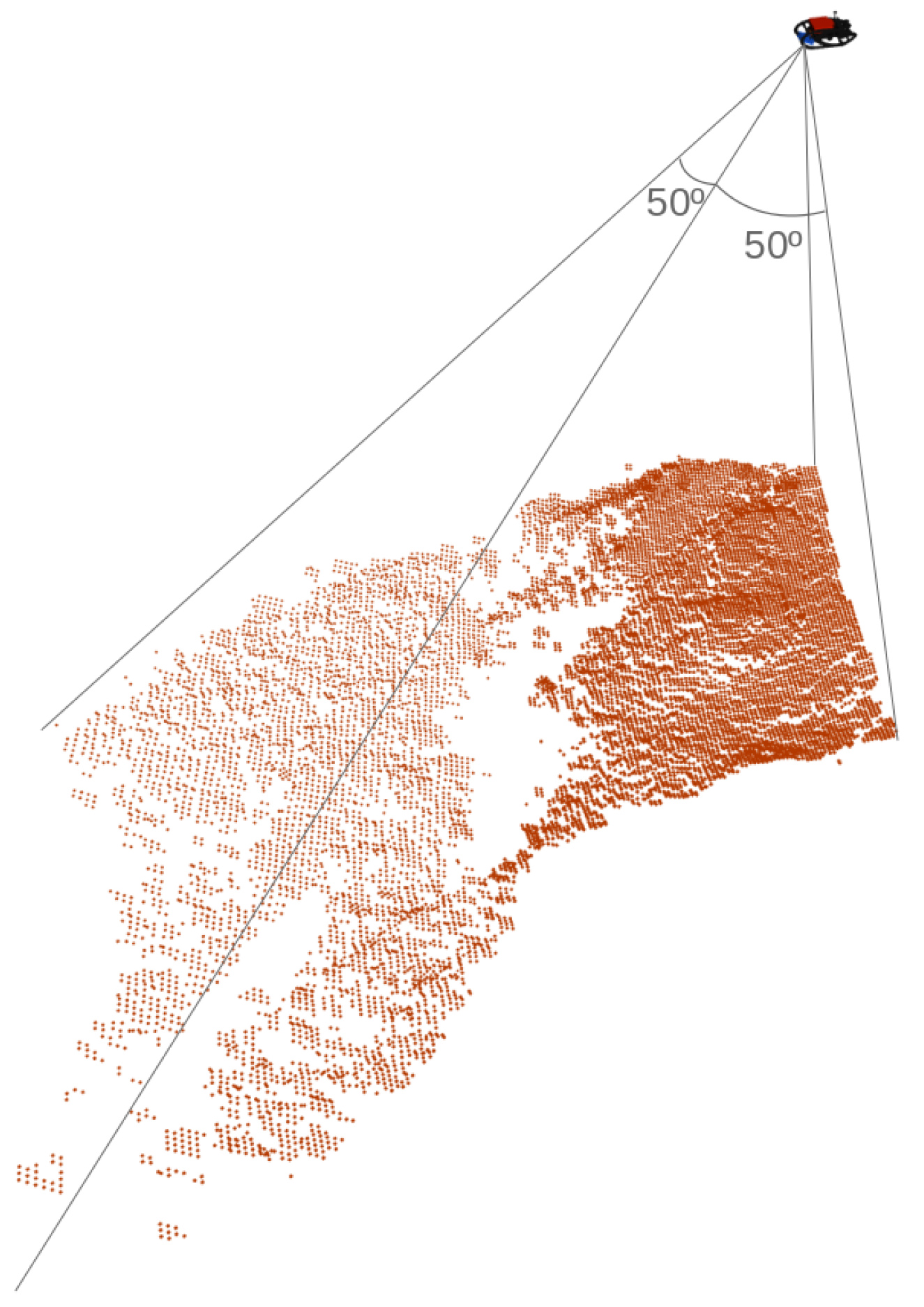
Figure 1 illustrates a single scan gathered from the Echoscope 3D profiling sonar. Each scan takes the form of a 128 by 128 matrix of range measurements, covering a seabed area inside the sonar field of view of 50 degrees in both along-track and across-track directions.
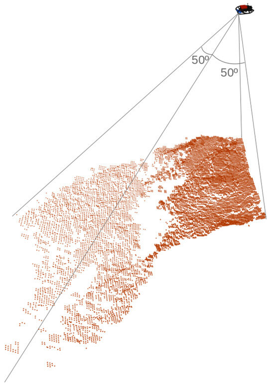
Figure 1.
Representation of a scan (red dots) captured by the Echoscope 3D sonar. The 3D model of the EVA AUV, where the sonar is assembled, is shown in the top right corner. The sonar field of view of 50º, in the along-track and across-track directions, is also illustrated.
2.1. Probabilistic Scan Modeling
To produce the probabilistic scan model, individual points are considered independent from each other. The ith scan point is represented by a multivariate Gaussian distribution , where is a three element vector containing the measured 3D coordinates, defined in the sonar reference frame s. The probabilistic model for the entire scan is the concatenation of all individual beams .
The covariance matrix for the ith beam is obtained by
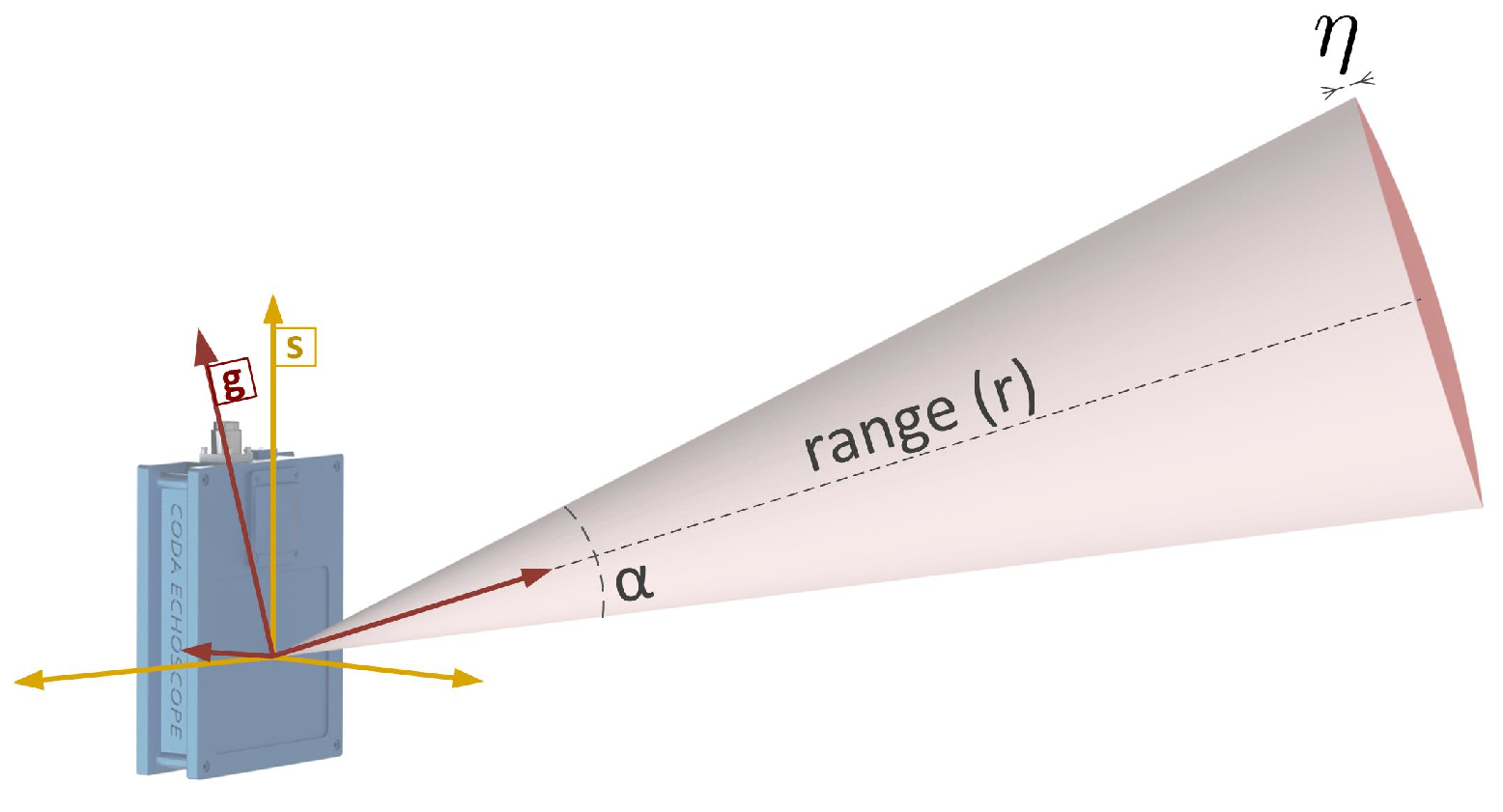
where is the covariance matrix in the beam’s reference frame g, and is the rotation matrix that transforms from g to s. The covariance matrix, , embodies the uncertainty associated with the conic beam shape. From Figure 2, two main sources of uncertainty impact the precision of the measurement: in the plane perpendicular to the beam direction, the insonification area increases as a function of the angular beam aperture and the slant range r; in the direction of the beam, the range error is a function of the intrinsic range resolution . Therefore, in the g reference frame, with the Z-axis passing through the center of the cone, the uncertainty is characterized by the following covariance matrix:

Figure 2.
Illustration of the conic beam shape from which the probabilistic beam model derives. For visualization purposes, the conical beam is depicted with an exaggerated aperture .
2.2. Probabilistic Scan Matching
Let us consider a reference scan , composed of m measurements, modeled according to our probabilistic sensor model and defined in the navigation reference frame n. Eventually, the robot moves, and a new scan is acquired. Let us refer to this new scan as the target scan , with o measurements, defined in the sonar reference frame s.
The displacement between scan acquisition poses is provided by an external localization algorithm. Taking advantage of the displacement estimate, the target scan can be transformed to the reference frame of the reference scan as follows:
where and define, respectively, the rotation matrix and translation vector from the sonar to the body reference frame b. These parameters, obtained through a previous calibration procedure, allow the beam to be transformed to the body frame . The transformation from the body to the navigation frame involves the rotation matrix and the translation vector , obtained from the current displacement estimate.
However, since the scan, the displacement and the extrinsic calibrations are inaccurate, as simply applying Equation (3) does not ensure the perfect alignment between both scans. The 3DupIC aims to refine this alignment and the associated robot displacement by repeating two steps until convergence. First, based on the Mahalanobis distance, point-to-point matches are established between scans. In the second stage, the Mahalanobis distance between associated point pairs is minimized.
2.2.1. Point Matching
For each point in the target scan, all points in are tested for similarity using the squared Mahalanobis distance:
where
represents the error between the jth reference point and the ith target point. The latter is projected into the n reference frame through function , defined in Equation (3). The covariance matrix , characterizing the matching uncertainty, is calculated using Equation (7).
The covariance matrices and represent the uncertainties of the scan point pairs, computed using Equation (4). Since the localization uncertainty affects the matching result, its contribution to the matching uncertainty is also considered: expression . The matrix is the Jacobian of the error function (Equation (6)) with respect to the displacement states, evaluated at the current estimate and at the scan point in the body frame . The matrix refers to the covariance matrix of the displacement estimate.
The Mahalanobis distance is assumed to be Gaussian; therefore, the squared Mahalanobis distance follows a chi-squared distribution , where q is the dimensionality of vector —which is, in this case, 3. A point is statistically compatible with a point if it passes the chi-squared test, i.e., the squared Mahalanobis distance is less than the inverse chi-squared cumulative function , evaluated for a given confidence level . Additionally, from the set of compatible points, only the one with a smaller Mahalanobis distance is selected. Therefore, a point pair is defined as
This search is repeated for all points in the target scan to build a set of point matches , where, for simplicity, represents the index pairing for the ith correspondence.
2.2.2. Optimization
The optimization step minimizes the squared Mahalanobis distances between corresponding points to obtain a refined displacement estimate:
3. Parallel Programming with OpenCL
The accelerated version of the 3DupIC was implemented using OpenCL—a cross-platform framework that abstracts the underlying hardware and enables parallel execution [20,21].
3.1. OpenCL Execution Model
Parallel programming is particularly suitable for problems that can be divided into smaller tasks to be executed simultaneously. In OpenCL, these self-contained functions are called kernels. The host program transmits orders to target devices using command queues, through which memory operations, kernel execution and synchronization commands are transmitted.
When launching a kernel, the host program must specify the size of the index space (work size), which corresponds to the number of kernel instances (work-items) to be executed. Each individual work-item is assigned with a unique global ID, based on the coordinates within the index space. In our application, taking, for example, a kernel to process each scan point individually, an index space of 16,384 is the most obvious solution, as it corresponds to the number of points in an Echoscope 3D scan. Additionally, the index space, also called NDRange in OpenCL, follows a N-dimensional arrangement, where . Returning to the previous example of an Echoscope 3D scan that takes the form of a matrix, a two-dimensional index space with a size of 128 in each dimension (total size of 16,384) provides a good fit.
All hardware poses a limit on the number of work-items that can be executed simultaneously. The assurance of simultaneous execution is only given for work-groups, which correspond to subsets of the total work size. The work-group size, also referred to as local size, can be specified at kernel launch time. Similarly, it is an N-dimensional space, with . Returning to the Echoscope 3D scan example, one could choose to form work-groups of 128 work-items to process each row of 128 sonar readings simultaneously. In this case, the definition of the local size should be 128 for the first dimension and 1 for the second dimension.
Each work-item has the ability to query its ID with respect to the global size and the local size using the get_global_id and get_local_id functions, respectively.
3.2. Memory Model
The OpenCL specification defines separate memory blocks for the host and the device, meaning that the host memory cannot be directly accessed by the device and vice versa. However, it is possible to transfer data using functions from the OpenCL API or through shared virtual memory. The workflow of a typical OpenCL application starts by copying the input data, usually stored at the host side, to the memory of the device. Once the processing is completed, the result is transferred in the opposite direction, i.e., from the device to the host.
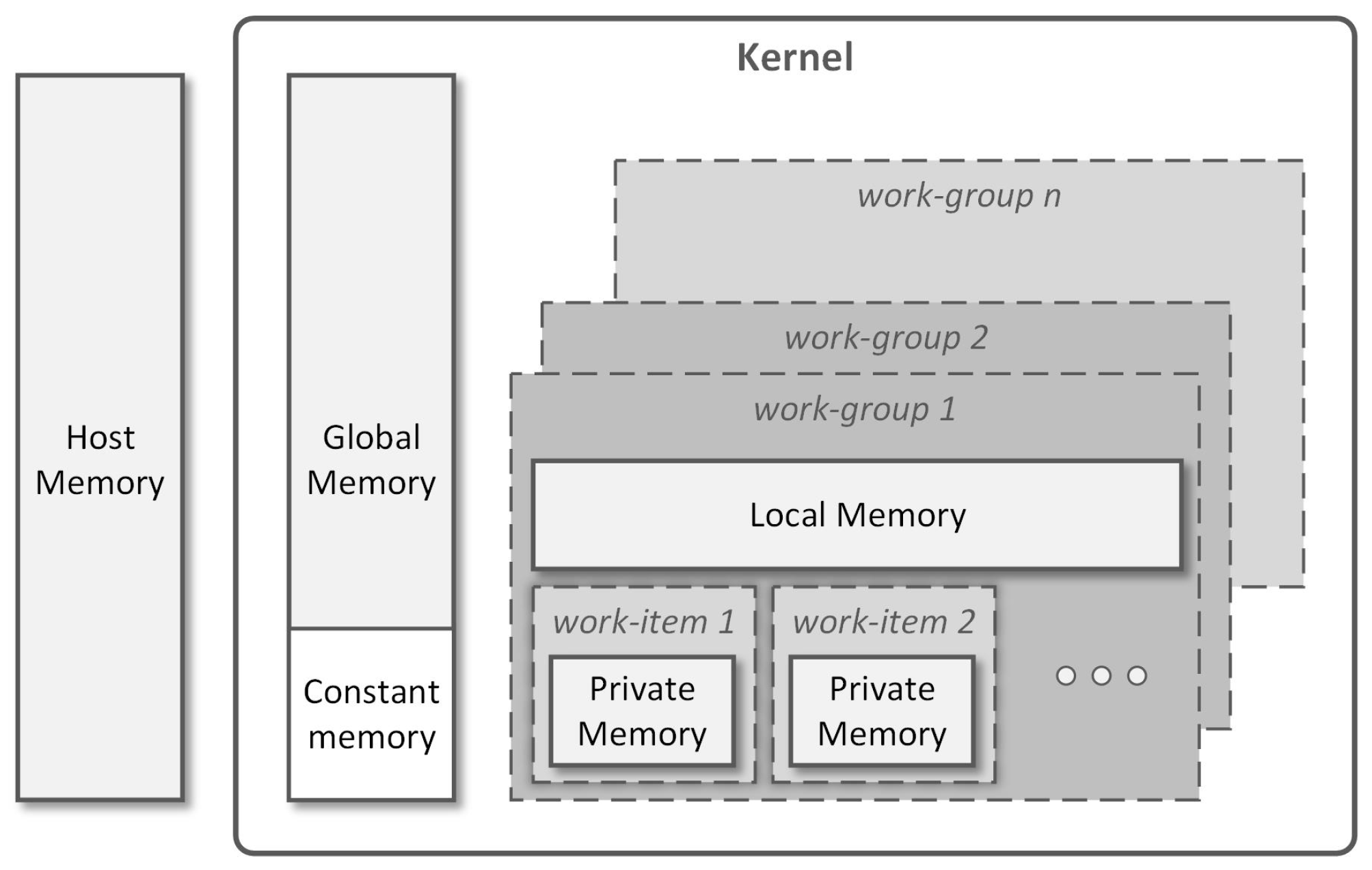
The OpenCL specification defines various memory regions available for the kernels running on the target device (Figure 3). A global memory block is shared between all processing units. It is normally the largest memory space but also the slowest. Allocations on this region are performed by the host at runtime, enabling data transfer between the host and the device. A constant memory region, available inside the global memory, stores read-only data from the device’s perspective. Only the host is allowed to write in the constant memory block. Each work-group is provided with a local memory block to be shared by the corresponding work-items. This is a low latency and high bandwidth memory region when compared to the global memory. Finally, a private memory region is available for each individual work-item. This is where local variables are stored. Within the kernel, keywords __global, __local and __constant are used to specify the region where variables are stored.

Figure 3.
Memory model for a kernel executing in the target device (adapted from [21]).
3.3. Programming Routines
The accelerated 3DupIC performs several calculations, involving matrix multiplication, matrix transpose and reductions. Next, a brief description of the parallel implementation of each of these operations is provided. It is important to mention that all operations outlined in this paper assume that matrices are stored in column-major order, so that the elements of a matrix A with m rows and n columns can be indexed in the following way:
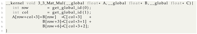
3.3.1. Matrix Multiplication
Consider the following matrix multiplication , where , and are square matrices:
To develop the matrix multiplication in a concurrent way, lets focus on the calculation of a single element. Taking, for example, , it is obtained by taking the dot product between the second row of B and the third column of C: . Replacing element indexes, assuming a column-major matrix ordering (Equation (13)), we obtain the following: . More generally, for the element in row i and column j, indexes can be defined as . Finally, the matrix multiplication can be obtained by repeating the previous operation for all elements of A. This is the same as repeating the kernel function nine times from Listing 1, launched with a 2D work size of .
| Listing 1. Matrix Multiplication Kernel. |
 |
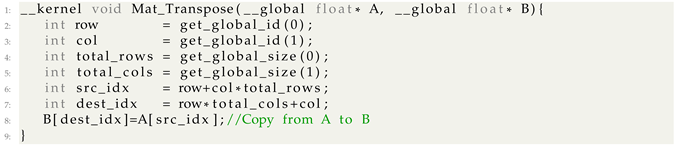
3.3.2. Matrix Transpose
The matrix transpose operation rearranges the matrix elements to produce a mirrored version across the diagonal:
This operation can be performed by simply swapping the element indexes: . A generic kernel function used to produce the index swap operation is provided in Listing 2. To transpose an m by n matrix, the kernel function should be launched with a two-dimensional NDRange and a total work size of . In this way, one work-item will be executed for each matrix element, producing the full inversion of the input matrix.
| Listing 2. Matrix Transpose Kernel. |
 |
3.3.3. Reduction
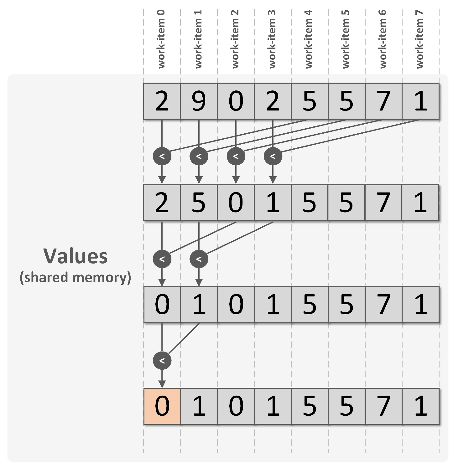
Parallel reduction operations are used to concurrently condense data into a single element using associativity binary operators. Typical problems solved with reductions include searching for the minimum or the maximum value inside an array, or summing all array elements. For a detailed explanation of reductions and practical recipes, the Raymond Tay’s book is recommended [22]. To illustrate the reduction operation, lets consider simple case of pre-initialized eight-element array (data), stored in the global memory block, from which we want to find the minimum value. Assume the reduction kernel is launched with a one-dimensional NDRange, imposing a work size of eight and a work-group size also equal to eight, which means that a total of eight work-items will be executed, all in the same work-group.
The parallel implementation to search for the minimum is provided in Listing 3. The algorithm is illustrated in Figure 4 to reveal the iterative nature of the reduction process.

Figure 4.
Illustration of a parallel reduction operation to find the minimum value of an eight-element array. Prior to the reduction itself, the eight work-items start by copying a single element value from the global to the local memory block, shared inside the work-group. Three comparison iterations are performed until the minimum value is stored in the first position of the shared array.
| Listing 3. Min() Reduction Kernel. |
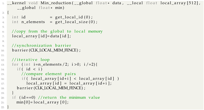 |
In a reduction, all work-items within a work-group cooperate to solve the problem, which implies the need for a shared memory area to store intermediate results. Local memory constitutes the best option in this particular case, as it is shared inside the work-group and provides fast access. Accordingly, the —second argument of the reduction kernel function (Listing 3)—is allocated for this purpose in the local memory region. In each iteration, multiple comparisons between element pairs are performed to select the minimum value of each pair. Only the element satisfying the search criteria passes to the next iteration. From one iteration to the next, half of the work-items become dormant, as a consequence of failing condition from line 14 in Listing 3. At the last iteration, the minimum value is stored in the first element of the shared array. The final result is written to the min variable by work-item index 0 (line 21 in Listing 3).
During the iterative process, the local_array is repeatedly read and written by different work-items. After writing operations (lines 7 and 17), the synchronization barriers from lines 10 and 18 stop the work-items inside the work-group until the barrier is reached by every work-item, ensuring the writing operations are finished before the work-items are allowed to continue.
3.3.4. Generic Matrix Multiplication
For small and fixed-size matrices, the multiplication operation can be easily hard-coded to be executed by a single work-item. Alternatively, a simple parallel implementation following Listing 1 is also possible. However, a new strategy is necessary to multiply large size matrices with a variable shape, as is often required by the 3DupIC. Please consider the following matrix multiplication case:
To compute Matrix A, a total of individual elements need to be calculated according to the following expression:
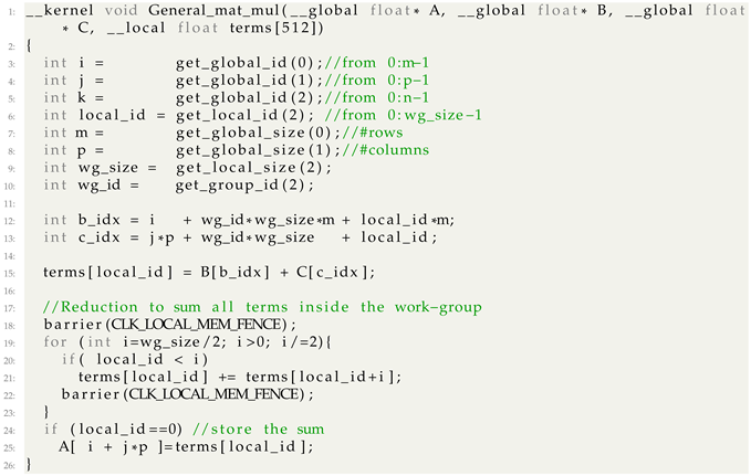
where is the element of A at row i and column j. According to (17), n multiplications are performed to calculate a single element of A. Therefore, the complexity of the generic matrix multiplication problem is . Accordingly, our kernel function (Listing 4) is designed to be launched with a three-dimensional NDRange of , where the first dimension indexes the matrix rows m, the second dimension indexes the matrix columns p, and the n multiplications, necessary to calculate each matrix element, are associated with the third dimension. Each individual work-item becomes responsible for computing a single term of the sum: (line 15, Listing 4). Finally, a reduction operation is performed (lines 18 to 25, Listing 4) to sum all partial terms and store the result (line 25, Listing 4). All indexes are computed according to (13).
The implementation presented in Listing 4 assumes a maximum work-group size of 512, meaning that only matrices with can be multiplied using this kernel. In fact, in the 3DupIC, this value is often exceeded. In those situations, a similar strategy can be used, but instead of storing the reduction value inside the final matrix, a larger size auxiliary matrix should be used to store this intermediate result. To complete the summation of the values stored in the auxiliary matrix, additional reductions should be performed until the value of is obtained.
| Listing 4. Generic Matrix Multiplication Kernel. |
 |
4. Accelerated 3DupIC
The parallel implementation of the 3DupIC algorithm is organized in two main blocks: the first group of kernel functions is concerned with finding compatible point matches between scans, performing all calculations between Equations (1) and (8); in the second step, a series of large matrix operations is executed to solve Equation (10).
4.1. Point Matching Step
The kernel functions concerned with finding the point matches between the target and reference scans are summarized in Table 1. Rows in the table specify the local and global work sizes applied for each kernel. The last column indicates the elements computed by the kernels, also referencing the equation used for their calculation.

Table 1.
Kernels used in the point matching step. The outputs are identified by the symbol and corresponding equation.
The first kernel entry in the table (Scan_initialization) is applied only once, as soon as a new target scan becomes available. Here, a simple outlier detection test is executed for each point to reject measurements very close to the sonar, within a threshold of 50 cm. Each Echoscope 3D scan usually contains a small amount of low range outlier measurements. This is the only filtering applied to the sonar scans during the entire process. Additionally, the probabilistic beam model is constructed for each measurement (Equation (2)), and extrinsic calibration parameters are applied to transform each beam from the sonar to the body reference frame, by partially applying Equations (3) and (4).
Subsequently, the algorithm enters an iterative cycle, where the robot displacement solution is consecutively refined. The Transform_scan kernel executes a work-item for each scan point to transform the beam model to the same reference frame of the reference scan. The last term of Equation (7) is also calculated.
Matching_part1 is assigned with a 2D work size of 16,384 × 16,384 to test all matching hypothesis by comparing each point from the target scan with all points in the reference scan. Each work-item computes the Mahalanobis distance (Equation (5)) and performs the statistic compatibility test (second term of Equation (8)). For each point in the target scan, all 16,384 points in the reference scan are evaluated, leading to 64 work-groups with 256 work-items per target scan point. A reduction is performed within the work-group to find the reference point with the smallest Mahalanobis distance. This brute-force search corresponds to the most heavy computation of the 3DupIC algorithm. From this process, 64 matching hypotheses are generated for each point in the target scan, requiring a second reduction using kernel Matching_part2 to find the matching pair.
4.2. Optimization Step
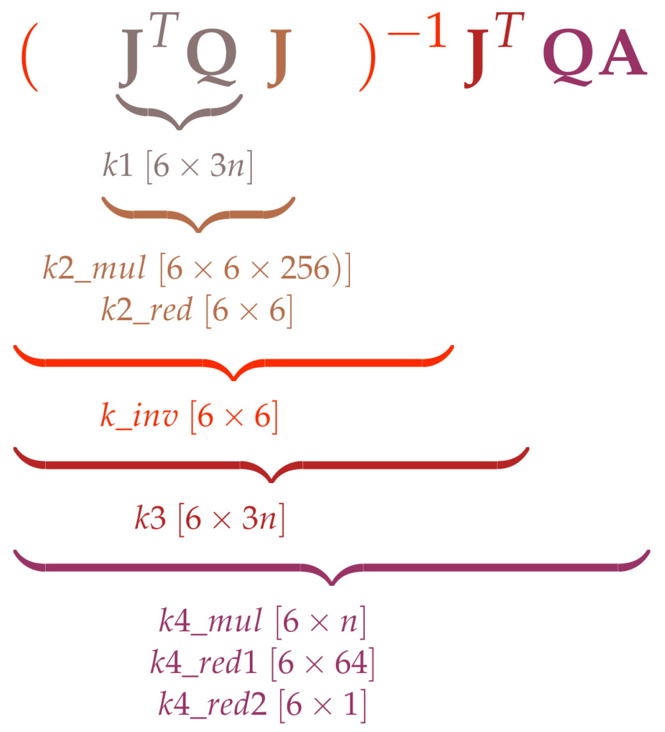
The optimization step computes the robot displacement that minimizes the Mahalanobis distance between previously established point matches, by solving the normal equation (Equation (10)). As most calculations consist of matrix multiplications and transpose operations, the generic kernel functions presented in the previous section are used here. A total of eight kernels are executed, as illustrated in Figure 5. The operations are executed sequentially, with the first multiplication being performed by kernel and producing a matrix, where n represents the number of point matched pairs. Kernel multiplies the result from kernel with matrix using the generic matrix multiplication kernel from Listing 4. A second reduction kernel () is necessary to sum all partial terms.
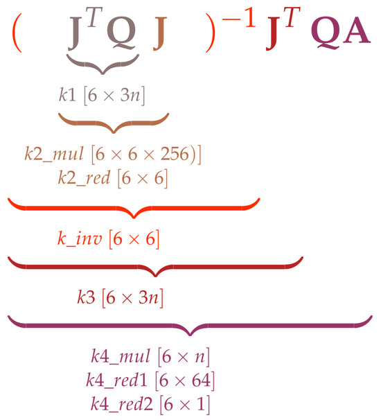
Figure 5.
Illustration of the kernel functions that, when applied sequentially, solve the normal equation. The values inside the square brackets represent the size of the output matrix produced by each kernel.
The inversion of the matrix is performed using the adjoint method implemented by kernel . The result of the inversion kernel is multiplied by , resulting in a matrix. Finally, the result from is multiplied by through kernel . The final solution is computed with two consecutive reductions (kernels and ) to perform a row-wise sum of the matrix produced by kernel .
5. Results
Considering that the Echoscope 3D sonar is usually carried by our EVA AUV, all experiments presented next were performed using an identical embedded computer to the one available onboard the real robot. The computer has an 11th Gen Intel Core i7-1185GRE processor, running a Fedora 38 distribution of the Linux operating system, and an integrated GPU Intel Iris Xe Graphics (TGL GT2) with OpenCL 3.0 support. To ensure realistic performance metrics, the algorithm was tested with real data, which were collected during field trials for the ¡VAMOS! project, held at the Silvermines flooded quarry in the Republic of Ireland.
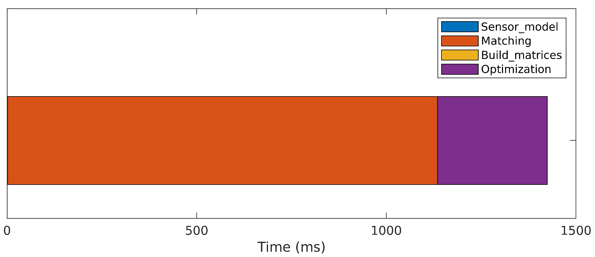
The results of a sequential version of the algorithm, executed on the CPU, are presented in Figure 6. Almost 1.5 s are necessary to perform a single iteration on average. The matching step, where all possible point matches between both scans are tested using the Mahalanobis distance, is the most expensive operation, consuming approximately 80% of the total iteration time. The optimization step, where large matrix manipulations are necessary to solve the normal equation (Equation (10)), spends most of the remaining time. The construction of the probabilistic sensor model (Equations (1)–(4)) and concatenations to build Matrices A, J and Q (Equations (11) and (12)) take negligible processing time.
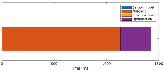
Figure 6.
Processing time required to perform a single iteration of the original 3DupIC method in a sequential manner on the CPU.
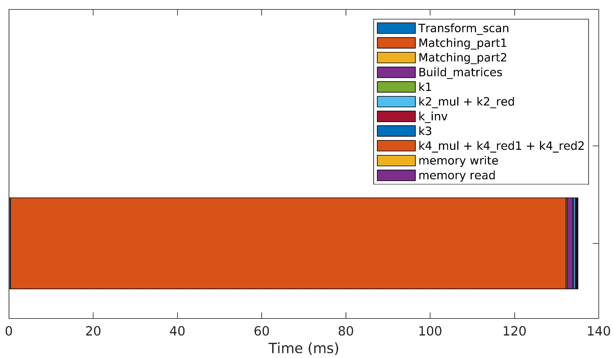
A tenfold speedup is achieved by the parallelized version, as depicted in Figure 7. The stacked bar plot shows the contribution of each kernel to the overall time necessary to execute a single iteration of the parallelized 3DupIC method. Each iteration takes just under 140 ms to execute, which is more than 10 times faster compared to the CPU experiment. Similarly to the sequential implementation, most of the time is spent on the matching step (98%). The matching operation performs a brute-force search, testing the compatibility of all points in the reference scan for each point in the target scan. This is a complex problem with over possible combinations. Significant acceleration is also observed in the optimization step, which i executed in under one millisecond.
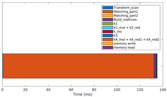
Figure 7.
Time spent on a single iteration of the original 3DupIC method when executed in a parallelized manner on the GPU.
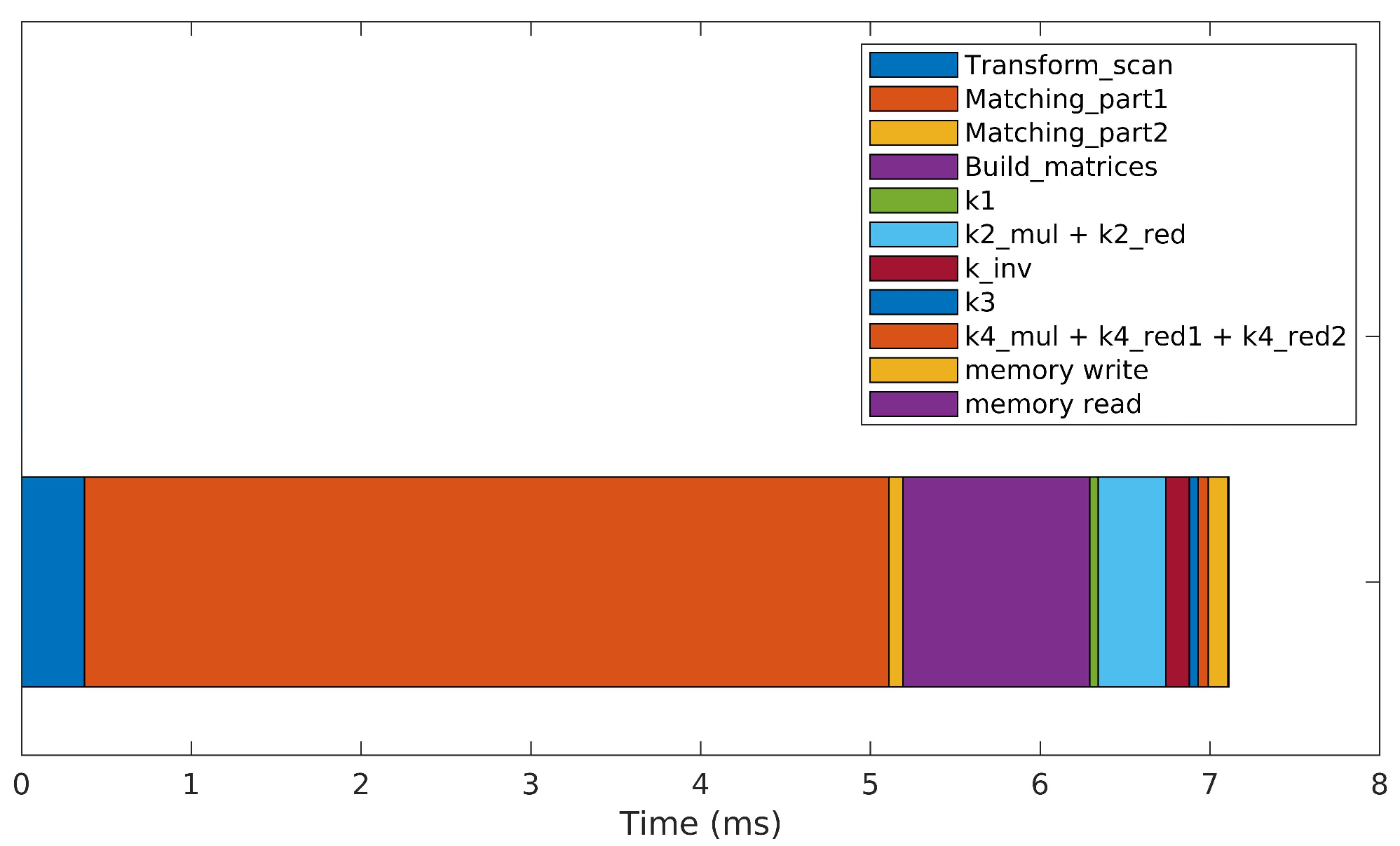
In an effort to further improve the algorithm’s performance, an optimized searching strategy was implemented, reducing the search to a small -point window. This search window is placed around the expected position where the matching point should lie, computed by geometrically transforming a given target point to the reference frame of the reference scan. This drastically reduces the computational load associated with the Matching_part1 kernel, leading to the processing times depicted in Figure 8. The optimized version takes around seven milliseconds to perform a single iteration, which constitutes a crucial improvement to reach real-time performance. The optimized implementation is 20 times faster than the brute-force approach and 200 times faster than the brute-force version running on the CPU.

Figure 8.
Processing time required to perform a single iteration of the optimized 3DupIC that reduces the matching point search to a small window of points.
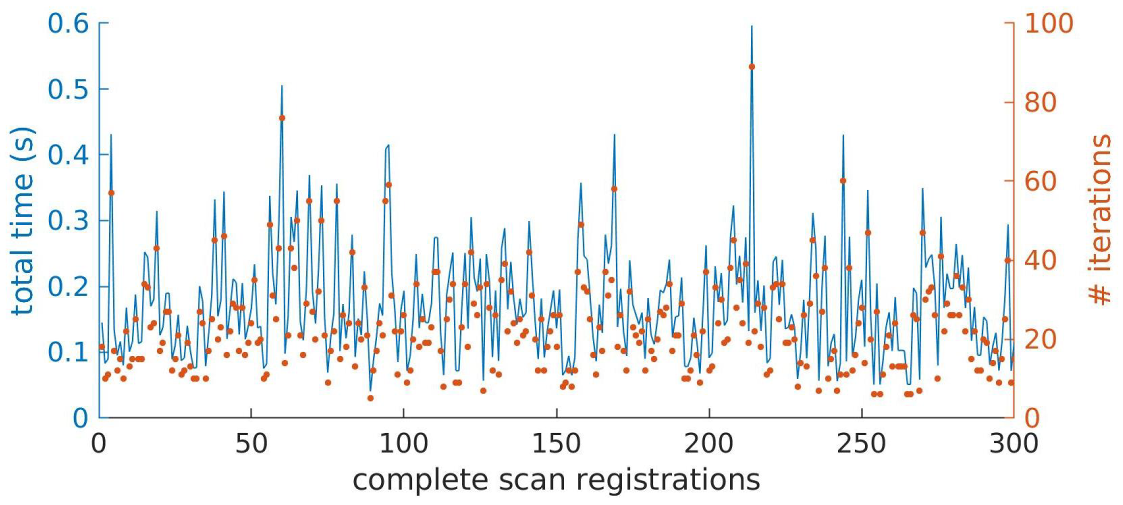
Figure 9 represents the total time and the number of iterations necessary to achieve convergence for 300 different scan registration cases, performed over a trajectory of approximately 150 m. The values where obtained for the optimized version of the algorithm, with the simplified matching approach. From the figure, a clear relation can be identified between the total processing time and the number of iterations performed. On average, 23.5 iterations and 0.1728 s are necessary to complete one scan registration, but these values can reach up to 0.6 ms for situations where the number of iterations approaches 90.
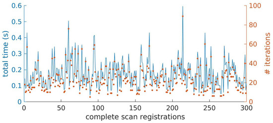
Figure 9.
Representation of the total time (left axis and line) and number of iterations (right axis and dots) necessary to perform 300 different scan registrations (horizontal axis).
Results demonstrate the capability of registering at least one key scan per second. Assuming a maximum surveying speed of 2 m per second, a new scan is registered every 2 m of displacement. For a surveying altitude of 2 m and a robot moving in a straight line at 2 m/s, the expected overlap between scans is approximately 66%. Therefore, even in this worst-case scenario, we can conclude that our parallel implementation of the 3DupIC method achieves real-time performance, so it can be executed onboard the EVA AUV during a real surveying mission.
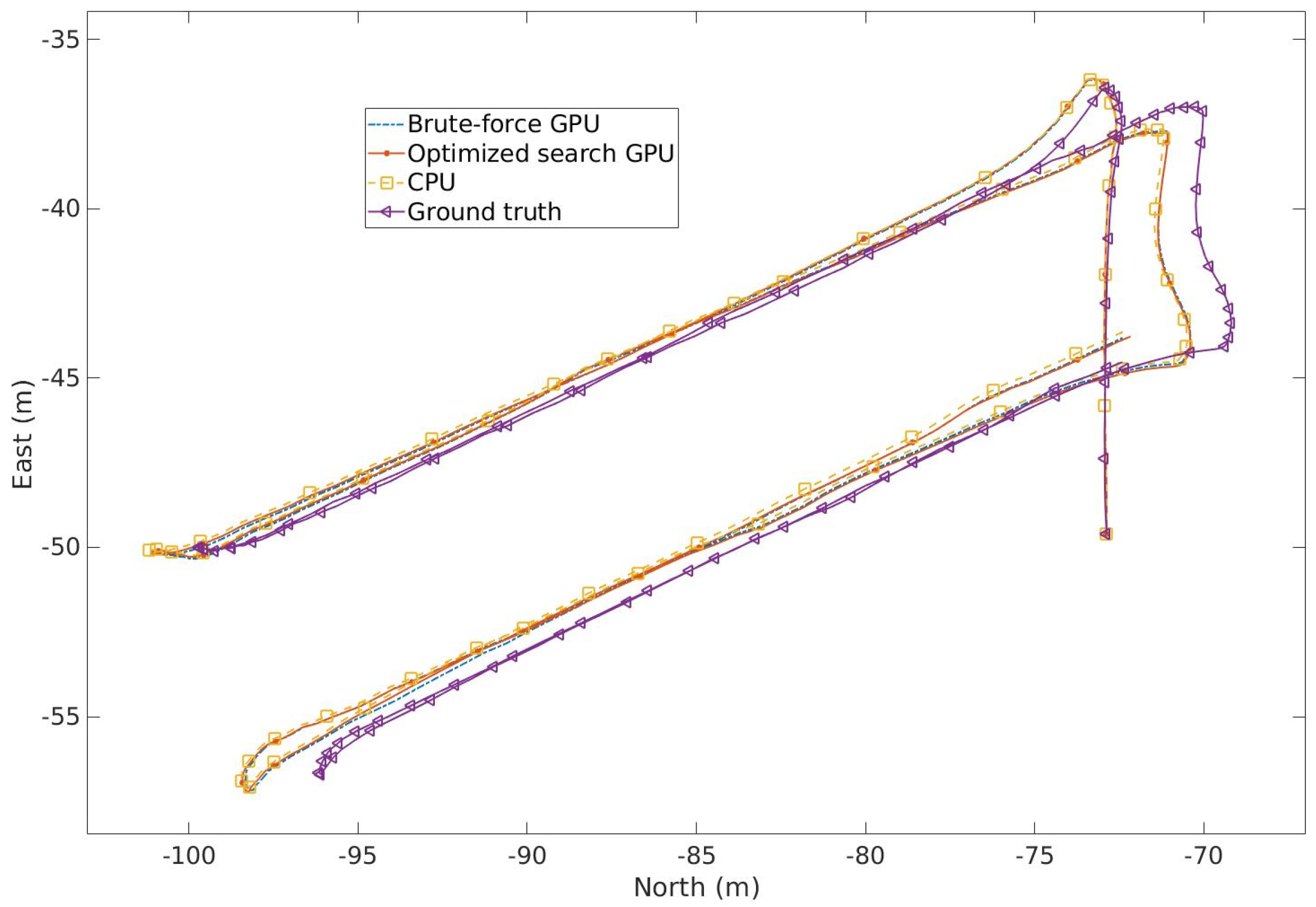
A detailed analysis of the 3DupIC registration accuracy can be found in [19] and is beyond the scope of this article. However, the illustration of the trajectories produced by the three variants (Figure 10) serves to demonstrate the consistency of the results. Although the trajectories produced by the three scan matching solutions are consistent, minor discrepancies can be observed. The deviations between the CPU produced trajectory and the parallelized versions are attributed to numerical approximations resulting from the use of single-precision data types in the GPU implementation. A slight difference is also observed between the trajectories of the parallelized versions, stemming from the different matching strategies used. Since the scan matching was used to register consecutive scans and no loops were closed, some degree of random walk is expected due to the aforementioned factors. The noticeable difference between the scan matching results and the ground truth trajectory is explained by the poor initialization of scan matching, particularly concerning the initial velocity of the vehicle due to low-quality DVL measurements.
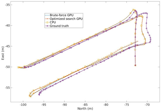
Figure 10.
Comparison between the trajectories produced by the reported implementations and the ground truth solution.
6. Conclusions
A collection of kernels for generic vector and matrix manipulation was presented. These building block easily adapt to vectors and matrices of different sizes, making them suitable for accelerating complex problems involving large-size vector and matrix operations. The adoption of the OpenCL framework facilitates code reusage due to its multi-platform support.
Taking advantages of the parallel processing kernels, an accelerated version of the 3DupIC algorithm was implemented. The results demonstrate the ability to achieve real-time performance, even when running the algorithm on a low-power integrated GPU. The optimized 3DupIC version simplifies the point matching task, running 20 times faster than the parallelized brute-force implementation and 200 times faster than the CPU implementation. The three methods produce similar trajectories with negligible random walk, which validates the simplified matching strategy.
To the authors’ knowledge, there is no other report of a scan matching method capable of registering 3D scans from an Echoscope sonar in six degrees of freedom and in real time. This advancement enables the use of the 3DupIC technique in future field operations, either to improve mapping consistency, provide relative localization corrections, or develop a SLAM process. A self-calibration procedure using scan matching is currently being developed to refine the transformation between the sonar and the body reference frame, aiming to enhance the global accuracy of the computed trajectories.
Author Contributions
Conceptualization, A.F.; methodology, A.F.; software, A.F.; validation, A.F., J.A., A.M. and E.S.; formal analysis, A.F., J.A., A.M. and E.S.; investigation, A.F., J.A., A.M. and E.S.; writing—original draft preparation, A.F. and J.A.; writing—review and editing, A.F., J.A., A.M. and E.S.; visualization, A.F.; supervision, A.M. and E.S.; project administration, J.A.; funding acquisition, J.A. and E.S. All authors have read and agreed to the published version of the manuscript.
Funding
This work was financed by national funds through the Portuguese funding agency, FCT - Fundação para a Ciência e a Tecnologia, within project UIDB/50014/2020. DOI:10.54499/UIDB/50014/ 2020|https://doi.org/10.54499/uidb/50014/2020 (accessed on 6 November 2024).
Data Availability Statement
Access to the dataset requires an explicit request to the corresponding author and subsequent approval.
Conflicts of Interest
The authors declare no conflicts of interest.
Abbreviations
The following abbreviations are used in this manuscript:
| 3D | Three-dimensional |
| 3DupIC | 3D underwater probabilistic iterative correspondence |
| API | Application programming interface |
| AUV | Autonomous underwater vehicle |
| CPU | Central processing unit |
| DVL | Doppler Velocity Log |
| GNSS | Global Navigation Satellite System |
| GPU | Graphics processing unit |
| ICP | Iterative closest point |
| IMU | Inertial motion unit |
| OpenCL | Open Computing Language |
| pIC | Probabilistic iterative correspondence |
| SLAM | Simultaneous localization and mapping |
References
- Zhang, B.; Ji, D.; Liu, S.; Zhu, X.; Xu, W. Autonomous Underwater Vehicle navigation: A review. Ocean. Eng. 2023, 273, 113861. [Google Scholar] [CrossRef]
- Majumder, S.; Scheding, S.; Durrant-Whyte, H. Sensor fusion and map building for underwater navigation. In Proceedings of the Australian Conference on Robotics and Automation, Melbourne, Australia, 30 August–1 September 2000; pp. 25–30. [Google Scholar]
- Chen, L.; Wang, S.; McDonald-Maier, K.; Hu, H. Towards autonomous localization and mapping of AUVs: A survey. Int. J. Intelligent Unmanned Syst. 2013, 1, 97–120. [Google Scholar] [CrossRef]
- Ferreira, A.; Matias, B.; Almeida, J.; Silva, E. Real-time GNSS precise positioning: RTKLIB for ROS. Int. J. Adv. Robot. Syst. 2020, 17, 172988142090452. [Google Scholar] [CrossRef]
- Almeida, J.; Matias, B.; Ferreira, A.; Almeida, C.; Martins, A.; Silva, E. Underwater Localization System Combining iUSBL with Dynamic SBL in ¡VAMOS! Trials. Sensors 2020, 20, 4710. [Google Scholar] [CrossRef] [PubMed]
- Besl, P.J.; McKay, N.D. A method for registration of 3-D shapes. IEEE Trans. Pattern Anal. Mach. Intell. 1992, 14, 239–256. [Google Scholar] [CrossRef]
- Rusinkiewicz, S.; Levoy, M. Efficient variants of the ICP algorithm. In Proceedings of the Third International Conference on 3-D Digital Imaging and Modeling, Quebec City, QC, Canada, 28 May–1 June 2001; pp. 145–152. [Google Scholar] [CrossRef]
- Vizzo, I.; Guadagnino, T.; Mersch, B.; Wiesmann, L.; Behley, J.; Stachniss, C. Kiss-icp: In defense of point-to-point icp–simple, accurate, and robust registration if done the right way. IEEE Robot. Autom. Lett. 2023, 8, 1029–1036. [Google Scholar] [CrossRef]
- Greenspan, M.; Yurick, M. Approximate k-d tree search for efficient ICP. In Proceedings of the Fourth International Conference on 3-D Digital Imaging and Modeling, Banff, AB, Canada, 6–10 October 2003; pp. 442–448. [Google Scholar] [CrossRef]
- Lu, F.; Milios, E. Robot pose estimation in unknown environments by matching 2D range scans. In Proceedings of the 1994 IEEE Conference on Computer Vision and Pattern Recognition, Seattle, WA, USA, 21–23 June 1994; pp. 935–938. [Google Scholar] [CrossRef]
- Zhang, Z. Iterative Point Matching for Registration of Free-form Curves and Surfaces. Int. J. Comput. Vis. 1994, 10, 119–152. [Google Scholar] [CrossRef]
- Minguez, J.; Lamiraux, F.; Montesano, L. Metric-Based Scan Matching Algorithms for Mobile Robot Displacement Estimation. In Proceedings of the 2005 IEEE International Conference on Robotics and Automation, Barcelona, Spain, 18–22 April 2005; pp. 3557–3563. [Google Scholar] [CrossRef]
- Torroba, I.; Bore, N.; Folkesson, J. A Comparison of Submap Registration Methods for Multibeam Bathymetric Mapping. In Proceedings of the 2018 IEEE/OES Autonomous Underwater Vehicle Workshop (AUV), Porto, Portugal, 6–9 November 2018; pp. 1–6. [Google Scholar] [CrossRef]
- Montesano, L.; Minguez, J.; Montano, L. Probabilistic scan matching for motion estimation in unstructured environments. In Proceedings of the 2005 IEEE/RSJ International Conference on Intelligent Robots and Systems, Edmonton, AB, Canada, 2–6 August 2005; pp. 3499–3504. [Google Scholar]
- Burguera, A. A novel approach to register sonar data for underwater robot localization. In Proceedings of the 2017 Intelligent Systems Conference (IntelliSys), London, UK, 7–8 September 2017; pp. 1034–1043. [Google Scholar] [CrossRef]
- Hernàndez Bes, E.; Ridao Rodríguez, P.; Ribas Romagós, D.; Batlle i Grabulosa, J. MSISpIC: A Probabilistic Scan Matching Algorithm Using a Mechanical Scanned Imaging Sonar. J. Phys. Agents 2009, 3, 3–11. [Google Scholar] [CrossRef]
- Zandara, S.; Ridao, P.; Mallios, A.; Ribas, D. MBpIC-SLAM: Probabilistic Surface Matching for Bathymetry Based SLAM. IFAC Proc. Vol. 2012, 45, 126–131. [Google Scholar] [CrossRef]
- Palomer, A.; Ridao, P.; Ribas, D. Multibeam 3D Underwater SLAM with Probabilistic Registration. Sensors 2016, 16, 560. [Google Scholar] [CrossRef] [PubMed]
- Ferreira, A.; Almeida, J.; Martins, A.; Matos, A.; Silva, E. 3DupIC: An Underwater Scan Matching Method for Three-Dimensional Sonar Registration. Sensors 2022, 22, 3631. [Google Scholar] [CrossRef] [PubMed]
- Stone, J.E.; Gohara, D.; Shi, G. OpenCL: A Parallel Programming Standard for Heterogeneous Computing Systems. Comput. Sci. Eng. 2010, 12, 66–73. [Google Scholar] [CrossRef]
- Kaeli, D.; Mistry, P.; Schaa, D.; Zhang, D. Heterogeneous Computing with OpenCL 2.0, 3rd ed.; Elsevier Science: Amsterdam, The Netherlands, 2015; ISBN 978-0128014141. [Google Scholar]
- Raymond, T. OpenCL Parallel Programming Development Cookbook; Packt Publishing Ltd.: Birmingham, UK, 2013; ISBN 978-1-84969-452-0. [Google Scholar]
Disclaimer/Publisher’s Note: The statements, opinions and data contained in all publications are solely those of the individual author(s) and contributor(s) and not of MDPI and/or the editor(s). MDPI and/or the editor(s) disclaim responsibility for any injury to people or property resulting from any ideas, methods, instructions or products referred to in the content. |
© 2025 by the authors. Licensee MDPI, Basel, Switzerland. This article is an open access article distributed under the terms and conditions of the Creative Commons Attribution (CC BY) license (https://creativecommons.org/licenses/by/4.0/).