
Estimating the Photovoltaic Potential of Building Facades and Roofs Using the Industry Foundation Classes

 ,
,
Abstract
:1. Introduction
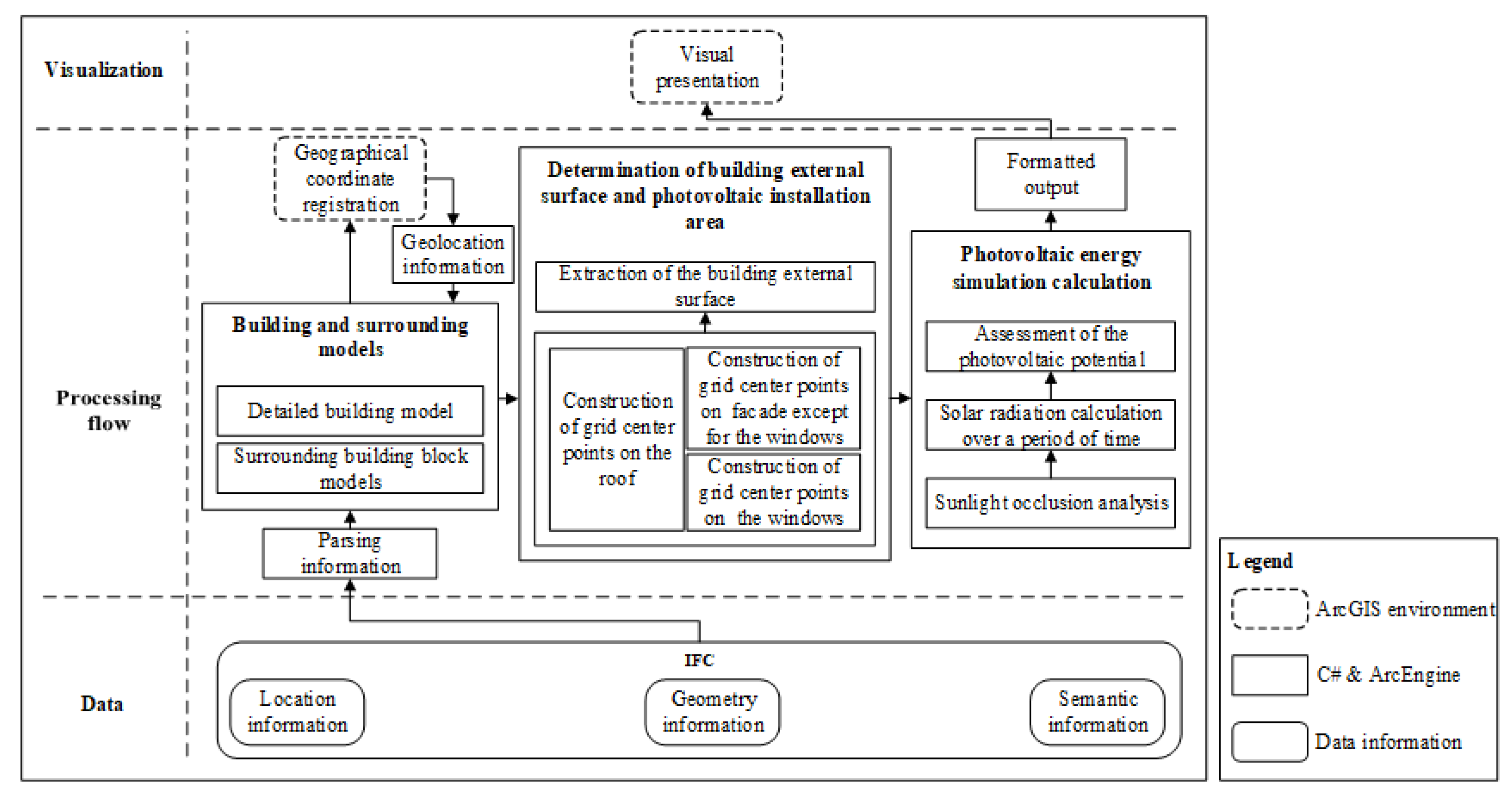
2. Methods
2.1. Analysis of IFC Data
2.2. Determination of Building External Surface and Photovoltaic Installation Area
2.3. Photovoltaic Energy Simulation Calculation
3. Simulation Results
3.1. Extraction of Available Installation Areas of the Building
3.2. Estimation of Photovoltaic Energy Generation Potential
4. Discussion
4.1. Comparison with Other Methods
4.2. Relationship between Calculation Time and Accuracy
5. Conclusions
Author Contributions
Funding
Institutional Review Board Statement
Informed Consent Statement
Data Availability Statement
Conflicts of Interest
References
- Cheng, L.; Xu, H.; Li, S.; Chen, Y.; Zhang, F.; Li, M. Use of LiDAR for calculating solar irradiance on roofs and facades of buildings at city scale: Methodology, validation, and analysis. ISPRS-J. Photogramm. Remote Sens. 2018, 138, 12–29. [Google Scholar] [CrossRef]
- Othman, A.R.; Rushdi, A.T. Potential of building integrated photovoltaic application on roof top of residential development in Shah Alam. Procedia-Soc. Behav. Sci. 2014, 153, 491–500. [Google Scholar] [CrossRef] [Green Version]
- Karteris, M.; Theodoridou, I.; Mallinis, G.; Papadopoulos, A.M. Facade photovoltaic systems on multifamily buildings: An urban scale evaluation analysis using geographical information systems. Renew. Sustain. Energy Rev. 2014, 39, 912–933. [Google Scholar] [CrossRef]
- Theodoridou, I.; Karteris, M.; Mallinis, G.; Papadopoulos, A.M.; Hegger, M. Assessment of retrofitting measures and solar systems’ potential in urban areas using Geographical Information Systems: Application to a Mediterranean city. Renew. Sustain. Energy Rev. 2012, 16, 6239–6261. [Google Scholar] [CrossRef]
- Liu, G.X.; Wu, W.X.; Ge, Q.S.; Dai, E.; Wan, Z.; Zhou, Y. A GIS method for assessing roof-mounted solar energy potential: A case study in Jiangsu, China. Environ. Eng. Manag. J. 2011, 10, 843–848. [Google Scholar]
- Kabir, M.H.; Endlicher, W.; Jägermeyr, J. Calculation of bright roof-tops for solar PV applications in Dhaka Megacity, Bangladesh. Renew. Energy 2010, 35, 1760–1764. [Google Scholar] [CrossRef]
- Fath, K.; Stengel, J.; Sprenger, W.; Wilson, H.R.; Schultmann, F.; Kuhn, T.E. A method for predicting the economic potential of (building-integrated) photovoltaics in urban areas based on hourly Radiance simulations. Sol. Energy 2015, 116, 357–370. [Google Scholar] [CrossRef]
- Strzalka, A.; Alam, N.; Duminil, E.; Coors, V.; Eicker, U. Large scale integration of photovoltaics in cities. Appl. Energy 2012, 93, 413–421. [Google Scholar] [CrossRef]
- Hofierka, J.; Kaňuk, J. Assessment of photovoltaic potential in urban areas using open-source solar radiation tools. Renew. Energy 2009, 34, 2206–2214. [Google Scholar] [CrossRef]
- Redweik, P.; Catita, C.; Brito, M. Solar energy potential on roofs and facades in an urban landscape. Sol. Energy 2013, 97, 332–341. [Google Scholar] [CrossRef]
- Szabó, S.; Enyedi, P.; Horváth, M.; Kovács, Z.; Burai, P.; Csoknyai, T.; Szabó, G. Automated registration of potential locations for solar energy production with Light Detection and Ranging (LiDAR) and small format photogrammetry. J. Clean. Prod. 2016, 112, 3820–3829. [Google Scholar] [CrossRef]
- Jakubiec, J.A.; Reinhart, C.F. A method for predicting city-wide electricity gains from photovoltaic panels based on LiDAR and GIS data combined with hourly Daysim simulations. Sol. Energy 2013, 93, 127–143. [Google Scholar] [CrossRef]
- Rodríguez, L.R.; Duminil, E.; Ramos, J.S.; Eicker, U. Assessment of the photovoltaic potential at urban level based on 3D city models: A case study and new methodological approach. Sol. Energy 2017, 146, 264–275. [Google Scholar] [CrossRef]
- Garnett, R.; Freeburn, J.T. Visual acceptance of library-generated citygml lod3 building models. Cartograph. Int. J. Geogr. Inf. Geovis. 2014, 49, 218–224. [Google Scholar] [CrossRef]
- Haala, N.; Kada, M. Panoramic scenes for texture mapping of 3D city models. In Proceedings of the ISPRS Working Group V/5: Panoramic Photogrammetry Workshop, Berlin, Germany, 24–25 February 2005; Volume 36. Part 5/W8. [Google Scholar]
- Grammatikopoulos, L.; Kalisperakis, I.; Petsa, E. Automatic Image Orientation for Accurate Texture Mapping of 3D City Models. In Proceedings of the International Conference ‘Science in Technology’ SCinTE, Athens, Greece, 5–7 November 2015. [Google Scholar]
- Biljecki, F.; Stoter, J.; Ledoux, H.; Zlatanova, S.; Çöltekin, A. Applications of 3D city models: State of the art review. ISPRS Int. Geo-Inf. 2015, 4, 2842–2889. [Google Scholar] [CrossRef] [Green Version]
- Wong, M.S.; Zhu, R.; Liu, Z.; Lu, L.; Peng, J.; Tang, Z.; Lo, C.H.; Chan, W.K. Estimation of Hong Kong’s solar energy potential using GIS and remote sensing technologies. Renew. Energy 2016, 99, 325–335. [Google Scholar] [CrossRef]
- Zhang, W.; Wong, N.H.; Zhang, Y.; Chen, Y.; Tong, S.; Zheng, Z.; Chen, J. Evaluation of the photovoltaic potential in built environment using spatial data captured by unmanned aerial vehicles. Energy Sci. Eng. 2019, 7, 2011–2025. [Google Scholar] [CrossRef] [Green Version]
- Azhar, S. Building information modeling (BIM): Trends, benefits, risks, and challenges for the AEC industry. Leadersh. Manag. Eng. 2011, 11, 241–252. [Google Scholar] [CrossRef]
- Wang, H.; Pan, Y.; Luo, X. Integration of BIM and GIS in sustainable built environment: A review and bibliometric analysis. Autom. Constr. 2019, 103, 41–52. [Google Scholar] [CrossRef]
- Pang, Y.Y.; Zhang, C.; Zhou, L.C.; Lin, B.X.; Lv, G.N. Extracting Indoor Space Information in Complex Building Environments. ISPRS Int. Geo-Inf. 2018, 7, 321. [Google Scholar] [CrossRef] [Green Version]
- Gimenez, L.; Robert, S.; Suard, F.; Zreik, K. Automatic reconstruction of 3D building models from scanned 2D floor plans. Autom. Constr. 2016, 63, 48–56. [Google Scholar] [CrossRef]
- Bahar, Y.N.; Pere, C.; Landrieu, J.; Nicolle, C. A thermal simulation tool for building and its interoperability through the building information modeling (BIM) platform. Buildings 2013, 3, 380–398. [Google Scholar] [CrossRef] [Green Version]
- Kamel, E.; Memari, A.M. Review of BIM’s application in energy simulation: Tools, issues, and solutions. Autom. Constr. 2019, 97, 164–180. [Google Scholar] [CrossRef]
- Li, H.X.; Ma, Z.L.; Liu, H.X.; Wang, J.; Al-Hussein, M.; Mills, A. Exploring and verifying BIM-based energy simulation for building operations. Eng. Constr. Archit. Manag. 2020, 27, 1679–1702. [Google Scholar] [CrossRef]
- Spiridigliozzi, G.; Pompei, L.; Cornaro, C.; Santoli, L.D.; Bisegna, F. BIM-BEM Support Tools for Early Stages of Zero-Energy Building Design; IOP Conference Series: Materials Science and Engineering; IOP Publishing: Bristol, UK, 2019; Volume 609, p. 072075. [Google Scholar]
- Salimzadeh, N.; Vahdatikhaki, F.; Hammad, A. BIM-based surface-specific solar simulation of buildings. ISARC. In Proceedings of the 35th International Symposium on Automation and Robotics in Construction, Berlin, Germany, 20–25 July 2018; IAARC Publications: Berlin, Germany, 2018; Volume 35, pp. 889–896. [Google Scholar]
- Salimzadeh, N.; Vahdatikhaki, F.; Hammad, A. Parametric modeling and surface-specific sensitivity analysis of PV module layout on building skin using BIM. Energy Build. 2020, 216, 109953. [Google Scholar] [CrossRef]
- Dimyadi, J.A.W.; Spearpoint, M.J.; Amor, R. Generating Fire Dynamics Simulator geometrical input using an IFC-based building information model. J. Inf. Technol. Constr. 2007, 12, 443–457. [Google Scholar]
- Laakso, M.; Kiviniemi, A.O. The IFC standard: A review of history, development, and standardization. J. Inf. Technol. Constr. 2012, 17, 134–161. [Google Scholar]
- Eastman, C.; Teicholz, P.; Sacks, R.; Liston, K. BIM Handbook: A Guide to Building Information Modeling for Owners, Managers, Designers, Engineers, and Contractors; John Wiley Sons, Inc.: Hoboken, NJ, USA, 2008. [Google Scholar]
- Kim, H.; Shen, Z.; Kim, I.; Kim, K.; Stumpf, A.; Yu, J. BIM IFC information mapping to building energy analysis (BEA) model with manually extended material information. Autom. Constr. 2016, 68, 183–193. [Google Scholar] [CrossRef]
- Deng, Y.; Cheng, J.C.; Anumba, C. Mapping between BIM and 3D GIS in different levels of detail using schema mediation and instance comparison. Autom. Constr. 2016, 67, 1–21. [Google Scholar] [CrossRef]
- Zhu, J.; Tan, Y.; Wang, X.; Wu, P. BIM/GIS integration for web GIS-based bridge management. Ann. GIS 2021, 27, 99–109. [Google Scholar] [CrossRef] [Green Version]
- Liu, Z.; Chen, K.; Peh, L.; Tan, K.W. A feasibility study of building information modeling for green mark new non-residential building (NRB): 2015 analysis. Energy Procedia 2017, 143, 80–87. [Google Scholar] [CrossRef]
- Lu, Y.; Wu, Z.; Chang, R.; Li, Y. Building Information Modeling (BIM) for green buildings: A critical review and future directions. Autom. Constr. 2017, 83, 134–148. [Google Scholar] [CrossRef]
- Lappalainen, K.; Valkealahti, S. Effects of PV array layout, electrical configuration and geographic orientation on mismatch losses caused by moving clouds. Sol. Energy 2017, 144, 548–555. [Google Scholar] [CrossRef]
- Rodrigo, P.; Velázquez, R.; Fernández, E.F.; Almonacid, F.; Pérez-Higueras, P.J. Analysis of electrical mismatches in high-concentrator photovoltaic power plants with distributed inverter configurations. Energy. 2016, 107, 374–387. [Google Scholar] [CrossRef]
- International Organization for Standardization. ISO TC184/SC4, ISO 10303-11:1994. In Industrial Automation Systems and Integration—Product Data Representation and Exchange—Part 11: Description Methods: The EXPRESS Language Reference Manual; International Organization for Standardization: Geneva, Switzerland, 1994. [Google Scholar]
- Angelis-Dimakis, A.; Biberacher, M.; Dominguez, J.; Fiorese, G.; Gadocha, S.; Gnansounou, E.; Guariso, G.; Kartalidis, A.; Panichelli, L.; Pinedo, I.; et al. Methods and tools to evaluate the availability of renewable energy sources. Renew. Sustain. Energy Rev. 2011, 15, 1182–1200. [Google Scholar] [CrossRef]
- Catita, C.; Redweik, P.; Pereira, J.; Brito, M.C. Extending solar potential analysis in buildings to vertical facades. Comput. Geosci. 2014, 66, 1–12. [Google Scholar] [CrossRef]
- Dubayah, R. Estimating net solar radiation using Landsat Thematic Mapper and digital elevation data. Water Resour. Res. 1992, 28, 2469–2484. [Google Scholar] [CrossRef]
- Fu, P.; Rich, P.M. Design and Implementation of the Solar Analyst: An Arcview Extension for Modeling Solar Radiation at Landscape Scales. In Proceedings of the Nineteenth Annual ESRI User Conference, San Diego, CA, USA, 26–30 July1999; Volume 1, pp. 1–31. [Google Scholar]
- Hay, J.E. Calculation of monthly mean solar radiation for horizontal and inclined surfaces. Sol. Energy 1979, 23, 301–307. [Google Scholar] [CrossRef]
- Hofierka, J.; Zlocha, M. A New 3-D solar radiation model for 3-D city models. Trans. GIS 2012, 16, 681–690. [Google Scholar] [CrossRef]
- Iqbal, M. An Introduction to Solar Radiation; Academic Press: New York, NY, USA, 1983. [Google Scholar]
- Kumar, L.; Skidmore, A.K.; Knowles, E. Modelling topographic variation in solar radiation in a GIS environment. Int. J. Geogr. Inf. Sci. 1997, 11, 475–497. [Google Scholar] [CrossRef]
- Liu, B.Y.H.; Jordan, R.C. The interrelationship and characteristic distribution of direct, diffuse and total solar radiation. Sol. Energy 1960, 4, 1–19. [Google Scholar] [CrossRef]
- Perez, R.; Seals, R.; Ineichen, P.; Stewart, R.; Menicucci, D. A new simplified version of the Perez diffuse irradiance model for tilted surfaces. Sol. Energy 1987, 39, 221–231. [Google Scholar] [CrossRef] [Green Version]
- Carl, C. Calculating Solar Photovoltaic Potential on Residential Rooftops in Kailua Kona, Hawaii; University of Southern California: Los Angeles, CA, USA, 2014. [Google Scholar]
- Lukač, N.; Žlaus, D.; Seme, S.; Žalik, B.; Štumberger, G. Rating of roofs’ surfaces regarding their solar potential and suitability for PV systems, based on LiDAR data. Appl. Energy 2013, 102, 803–812. [Google Scholar] [CrossRef]
- Lukač, N.; Žalik, B. GPU-based roofs’ solar potential estimation using LiDAR data. Comput. Geosci. 2013, 52, 34–41. [Google Scholar] [CrossRef]
- Zheng, Y.; Weng, Q. Assessing solar potential of commercial and residential buildings in Indianapolis using LiDAR and GIS modelling. In Proceedings of the 2014 Third International Workshop on Earth Observation and Remote Sensing Applications (EORSA), Changsha, China, 11–14 June 2014; IEEE: Piscataway, NJ, USA, 2014; pp. 398–402. [Google Scholar]
- Duffie, J.A.; Beckman, W.A. Solar Engineering of Thermal Processes; Wiley: New York, NY, USA, 1991. [Google Scholar]
- Kreith, F.; Kreider, J.F. Principles of Solar Engineering; Hemisphere Publishing Corp.: Washington, DC, USA, 1978. [Google Scholar]
- Gul, M.S.; Muneer, T.; Kambezidis, H.D. Models for obtaining solar radiation from other meteorological data. Sol. Energy 1998, 64, 99–108. [Google Scholar] [CrossRef]
- Kasten, F.; Czeplak, G. Solar and terrestrial radiation dependent on the amount and type of cloud. Sol. Energy 1980, 24, 177–189. [Google Scholar] [CrossRef]
- Cartwright, T.J. Modeling the World in a Spreadsheet: Environmental Simulation on a Microcomputer; Johns Hopkins University Press: Baltimore, MD, USA, 1993. [Google Scholar]
- Gates, D.M. Biophysical Ecology; Springer: New York, NY, USA, 1980. [Google Scholar]
- Schallenberg-Rodríguez, J. Photovoltaic techno-economical potential on roofs in regions and islands: The case of the Canary Islands: Methodological review and methodology proposal. Renew. Sustain. Energy Rev. 1980, 20, 219–239. [Google Scholar] [CrossRef]
- Panasonic. Solar Power Generation System for Residential Use. Homes and Living. 2014. Available online: http://sumai.panasonic.jp/catalog/solar.html (accessed on 1 May 2021).
- Yuan, J.; Farnham, C.; Emura, K.; Lu, S. A method to estimate the potential of rooftop photovoltaic power generation for a region. Urban Clim. 2016, 17, 1–19. [Google Scholar] [CrossRef]
- Carneiro, C.; Morello, E.; Desthieux, G.; Golay, F. Urban Environment Quality Indicators: Application to Solar Radiation and Morphological Analysis on Built Area. In Proceedings of the 3rd WSEAS International Conference on Visualization, Imaging and Simulation. World Scientific and Engineering Academy and Society (WSEAS), Faro, Portugal, 3–5 November 2010; pp. 141–148. [Google Scholar]
- NASA. 2019. Available online: https://ladsweb.modaps.eosdis.nasa.gov/ (accessed on 5 July 2020).
- Gimenez, L.; Hippolyte, J.L.; Robert, S.; Suard, F.; Zreik, K. Review: Reconstruction of 3D building information models from 2D scanned plans. J. Build. Eng. 2015, 2, 24–35. [Google Scholar] [CrossRef]
- Volk, R.; Stengel, J.; Schultmann, F. Building Information Modeling (BIM) for existing buildings—Literature review and future needs. Autom. Constr. 2014, 38, 109–127. [Google Scholar] [CrossRef] [Green Version]
- Ledoux, H.; Meijers, M. Extruding building footprints to create topologically consistent 3D city models. In Urban and Regional Data Management. UDMS Annual; Krek, A., Rumor, M., Zlatanova, S., Fendel, E., Eds.; CRC Press: Boca Raton, FL, USA, 2009; pp. 39–48. [Google Scholar]


| Building Element | Actual Area (m2) | Industry Foundation Classes (IFC) Extraction Area (m2) | Available Installation Area (m2) | Proportion of Available Area (%) |
|---|---|---|---|---|
| Roof | 783.48 | 783.48 | 755 | 96.36 |
| Facade (excluding windows) | 17,399.79 | 17,399.79 | 6659 | 38.27 |
| Windows | 2726.37 | 2726.37 | 1581 | 57.99 |
| Entire building (excluding windows) | 18,183.27 | 18,183.27 | 7414 | 40.77 |
| Entire building | 20,909.64 | 20,909.64 | 8995 | 43.02 |
| Time Period | Photovoltaic Energy Generation (MWh) | Time Period | Photovoltaic Energy Generation (MWh) |
|---|---|---|---|
| January | 38.51 | October | 91.45 |
| February | 59.55 | November | 53.79 |
| March | 97.55 | December | 35.48 |
| April | 120.59 | Spring | 342.99 |
| May | 102.78 | Summer | 346.93 |
| June | 119.94 | Autumn | 194.51 |
| July | 122.22 | Winter | 170.25 |
| August | 116.23 | Annual | 1054.69 |
| September | 99.84 |
| Method | Semantic Information | Data Acquisition Difficulty | Accuracy | Information Integrity | Extracted Building Elements |
|---|---|---|---|---|---|
| Industry Foundation Classes (IFC) | Yes | Medium | High | High | Roof, Facade, Window |
| Direct extruding | No | Easy | Low | Low | Roof, Facade |
| High-definition image | No | Medium | Low | Low | Roof |
| Point cloud data | No | Difficult | High | Medium | Roof, Facade |
Publisher’s Note: MDPI stays neutral with regard to jurisdictional claims in published maps and institutional affiliations. |
© 2021 by the authors. Licensee MDPI, Basel, Switzerland. This article is an open access article distributed under the terms and conditions of the Creative Commons Attribution (CC BY) license (https://creativecommons.org/licenses/by/4.0/).
Share and Cite
Lu, X.; Li, G.; Wang, A.; Xiong, Q.; Lin, B.; Lv, G. Estimating the Photovoltaic Potential of Building Facades and Roofs Using the Industry Foundation Classes. ISPRS Int. J. Geo-Inf. 2021, 10, 827. https://doi.org/10.3390/ijgi10120827
Lu X, Li G, Wang A, Xiong Q, Lin B, Lv G. Estimating the Photovoltaic Potential of Building Facades and Roofs Using the Industry Foundation Classes. ISPRS International Journal of Geo-Information. 2021; 10(12):827. https://doi.org/10.3390/ijgi10120827
Chicago/Turabian StyleLu, Xiu, Guannan Li, Andong Wang, Qingqin Xiong, Bingxian Lin, and Guonian Lv. 2021. "Estimating the Photovoltaic Potential of Building Facades and Roofs Using the Industry Foundation Classes" ISPRS International Journal of Geo-Information 10, no. 12: 827. https://doi.org/10.3390/ijgi10120827
APA StyleLu, X., Li, G., Wang, A., Xiong, Q., Lin, B., & Lv, G. (2021). Estimating the Photovoltaic Potential of Building Facades and Roofs Using the Industry Foundation Classes. ISPRS International Journal of Geo-Information, 10(12), 827. https://doi.org/10.3390/ijgi10120827