Abstract
As communication technology and smartphones develop, many indoor positioning applications based on Bluetooth low energy (BLE) beacons have emerged. However, in a complex BLE network, it can be challenging to select the optimal reference beacon, and accurate positioning becomes difficult. Fortunately, if the BLE network is displayed on a map, we can intuitively grasp the structure and density of the beacons in each area, which is important information for accurate positioning. Therefore, in this study we developed a map-aided indoor positioning algorithm to model the relationship between beacons in the positioning area in a parking lot. Specifically, the algorithm split all beacons into multiple cell areas to find the optimal reference beacon in that area. Then, the optimal reference beacon is used to find the preferred reference beacons among the real-time beacons. Finally, the positioning results were calculated and evaluated according to the preferred beacons. According to the results, our method can optimize the selection of reference beacons in different areas. The average positioning accuracy was 2.09 m and the results can be scored accurately. The results verify that our algorithm can effectively use map information to guide the selection of reference beacons in complex environments.
1. Introduction
The development and popularization of communication technology have allowed the integration of indoor positioning technologies in smartphones [1,2,3,4]. The positioning services can be used for multiple purposes such as finding cars in underground parking lots [5] and shopping in retail stores [6]. However, owing to complex indoor environments, using a single technology to achieve positioning in various places is a challenging concept. Indoor positioning methods using multiple technologies such as Wi-Fi, Bluetooth, and audio have emerged [7] to cater to varying requirements. In various technologies, smartphones can directly obtain Bluetooth low energy (BLE) signals using BLE beacons that can have separate batteries. The characteristics of low cost and simple deployment have popularized BLE beacons as a positioning solution for mobile phones [8,9,10]. In addition, BLE beacon deployment rules are free, and different structures and densities can be deployed according to requirements. This enables range-based positioning technology to achieve good results [10].
Indoor positioning and maps are usually used in conjunction to display positioning results to users. The user’s position in the scene is visually displayed by projecting the results onto the indoor map. Furthermore, integrating positioning technology with maps can provide improved indoor location services, such as check-in, indoor navigation, and other services [2]. Map information can effectively constrain positioning results and paths, and is used in many areas of research to improve positioning results. In terms of positioning constraints, mapping elements such as doors and walls is critical to restrict and correct unreasonable results. Map information has been primarily applied to perform post-processing operations after acquiring positioning results. For example, using wall constraints to avoid positioning trajectories through the wall [11,12,13], and utilizing basic heading information of buildings to reduce heading errors [14,15]. In terms of path constraints, it is critical to understand the relationship between topological connections and paths, and correct path deviations. To achieve this, previous studies have estimated the user’s route from the location estimation results, then considered the building’s passable areas to construct a link node topology map to correct the estimated route [16,17]. However, this method contains two processes of location estimation and trajectory estimation, which can easily lead to errors [18]. Yamamoto et al. proposed that the received signal strength indicator (RSSI) of BLE can be combined with map information to directly estimate the global optimal path [18]. This method does not require position estimation, and effectively improves the accuracy.
Different from the constraints of the map on the positioning results and trajectory in the existing research, we found that map information also has a constraint on the beacons. When the beacons are displayed on a map, the distribution and connectivity of the beacons are clear at a glance. For example, we can directly see which areas are more densely distributed and where the distribution is more reasonable. If this information can be modeled as prior knowledge, the beacon selection and result evaluation during positioning can be optimized. Thus, in practice, the usability of the positioning algorithm can be enhanced. On the one hand, the best combination of reference beacons can be selected in different areas. On the other hand, different beacon deployment structures and densities are given different evaluations. For example, densely deployed areas usually get better positioning results than sparse areas and so are evaluated as better.
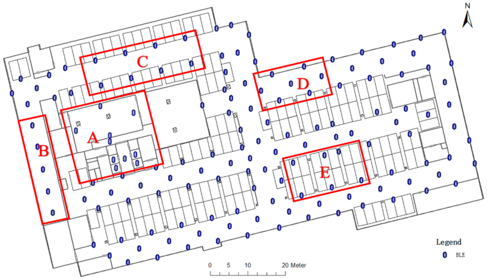
In an ideal experimental environment, when beacons were deployed in a regular structure and reasonable spacing, optimal results were usually achieved [19]. However, in real-world conditions, the physical environment is usually more complicated, which results in beacons not being deployed according to target rules and the disruption of signals. For these reasons, the signal composition for real-time positioning is extremely complicated. Figure 1 shows the actual deployment of BLE beacons in an underground parking lot. The deployment of beacons and the signal coverage in each region were different. Theoretically, the density and structure of Area-D are optimal, and the best positioning accuracy can be obtained. However, the deployments Area-A and -B are not suitable for the trilateration positioning algorithm. Modeling the algorithm to select the appropriate beacon and algorithm for positioning according to the beacons around the device greatly affects the positioning effect in practical applications.
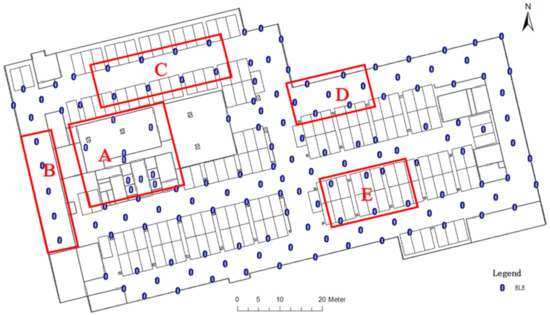
Figure 1.
Deployment of BLE beacons with different densities and spatial layouts in underground parking lots: Area-A is the deployment of rooms and elevators, Area-B is a straight-line deployment for the tunnel, Area-C is deployed on two pillars, Area-D is a cross deployment on both sides of the road, and Area-E is a symmetrical deployment above the parking space.
Owing to the complex structure of beacon deployment, it is difficult to determine a suitable positioning method and evaluate the availability of beacons from only real-time beacon sequences. This paper proposes a positioning method for BLE beacons aided by map information and improves the positioning effect by selecting appropriate reference beacons and positioning algorithms. The visual relationship between adjacent beacons in the area is modeled through a combination of map information and BLE location; a large positioning area is divided into multiple small cell areas with their respective layout shapes (points, lines, and polygons). Each cell area has a set of optimal reference beacons whose combinations are constructed using spatial relationships. A BLE beacon signal coverage rating map is constructed and divided into high, medium, and low levels to quantify the BLE beacon coverage of each cell area. In the positioning stage, sequences with severe signal fluctuations are eliminated according to the degree of suitability of the received signal strength indicator (RSSI) ranking of real-time beacons and their distribution in the actual space. Next, a reference beacon is selected from the relatively stable beacon sequences for positioning. Experiments demonstrate that this method can effectively improve positioning in a complex beacon deployment environment. Thus, a complete positioning algorithm framework is developed. The algorithm can determine the cell area based on the real-time beacon sequence and can accurately select the appropriate algorithm and reference beacon to improve positioning.
Section 2 introduces related research on BLE positioning and map-added positioning. Section 3 describes the composition of the algorithm in detail. Section 4 describes the experimental setup and the results. Section 5 discusses the algorithm and experimental performance of this study, and finally summarizes the work of this paper and provides suggestions for future research.
2. Related Research
Current approaches to indoor localization can be categorized as infrastructure-based and infrastructure-less [20]. Infrastructure-based approaches usually require existing infrastructures such as WIFI and BLE, and the use of smartphones to receive the RSSI of the beacon to achieve positioning [21]. The RSSI reflects the distance between the device and the beacon. However, since RSSI is easily affected by environmental obstacles and multipath factors [21,22,23], a filtering algorithm is usually required [24,25,26] to enhance the accuracy of RSSI. In addition, the deployment structure of the beacons also greatly affects the availability of RSSI [27]. Increasing the deployment density of beacons can ensure that sufficient reference beacons are within the visual range of the device [28]. Moreover, high density will cause significant cross-talk between the beacons [29].
Due to the complexity of the actual signal environment, the optimal selection of reference beacons or positioning algorithms is useful for accurate positioning [30,31,32,33]. The approximate point-in-triangulation (APIT) algorithm [32] starts from the position of the beacon, and decides whether to filter the reference beacon by judging whether the unknown node is located in a triangle formed by any three beacons, the accuracy is greatly improved compared to before the optimization. Orujov et al. compared several positioning algorithms, then proposed and implemented a fuzzy logic based scheme to select the most fitting algorithm depending upon the size of the room, the number of beacons available and the strength of the signal [33]. In follow-up research, they further used fuzzy logic type-2 to optimize the fingerprint positioning algorithm [20]. This method obtained an average positioning accuracy of 0.43 m, which also verified the high applicability of the fingerprint positioning algorithm. Existing studies have shown that selecting appropriate positioning algorithms and reference beacons can effectively improve positioning accuracy. However, there is still a lack of effective application of prior information such as the spatial distribution relationship of beacons. In this study, we modeled the spatial relationship of beacons in a scene, and explored how this type of information can be used for the optimization of beacons and positioning algorithms.
Infrastructure-less approaches require no support from the existing infrastructure. For example, some studies use the built-in sensor of mobile phones to achieve the continuous positioning of pedestrians [34,35] or use geomagnetism for fingerprint positioning [3]. In the realization of continuous positioning, algorithms such as Kalman filter [12] and particle filter [11,13] are usually used to achieve the fusion of different positioning methods. Indoor maps are used to constrain the emergence of problems such as wall penetration during the fusion process [11,12,13,36]. Wang et al. proposed a maximum likelihood particle filter algorithm, which merges the particle prediction and updates steps into a single step, and avoids the waste of unnecessary particles as in the classic particle filter algorithm [37]. However, the constraint effect of the map information on the reference beacon is rarely studied. By using the relationship between the scene and the beacon, the rationality of the combination of beacons can be restricted. For example, in a room, the beacon combination with the strongest RSSI is usually the beacon deployed inside the room. Here, we investigated the constraints the map information has on the combination of reference beacons, and how the independent reference beacons are used in beacon combinations.
3. Research Method
3.1. Overview
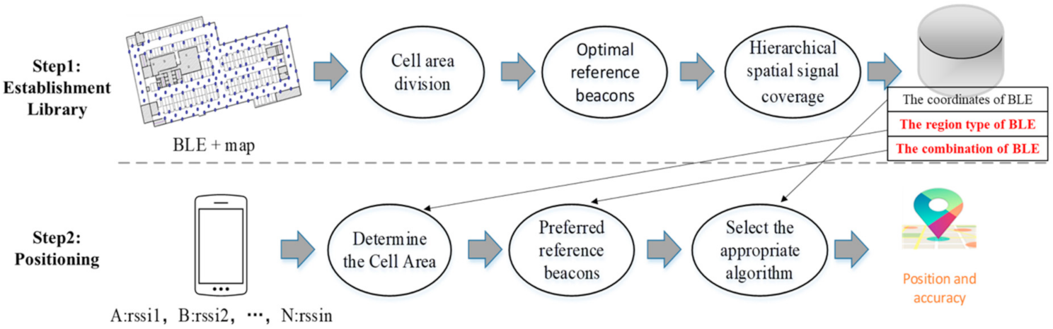
The framework of the proposed method is shown in Figure 2. The method consists of two parts: establishment library and positioning. In the establishment library phase, map information and BLE are used to divide the positioning area into multiple cell areas, and each area has a set of optimal reference beacons. Previously independent beacons will be optimally combined for positioning. In the positioning phase, the real-time beacon sequence is used to determine the cell area to which the device belongs. The optimal beacon combination is used to select reference beacons from real-time beacons to achieve accurate positioning. The procedure of the whole algorithm framework is described in Algorithm 1.
| Algorithm 1 Proposed localization algorithm. |
|

Figure 2.
The whole algorithm workflow. The thick arrow is the algorithm flow and the thin arrow indicates the specific information mainly used in the operation.
3.2. Establish-Library
The establishment library mainly divides the entire area into multiple cell areas, and each cell area has its optimal reference beacon combination, layout, density, etc.
3.2.1. Cell Area Division
Map Information
Map information is usually used to mark out the BLE settings location, or used to assist in constraining the positioning results [3,11,12,13]. However, the map information can also constrain the relationship between beacons and assist in the division of areas. When there is insufficient map information, the BLE beacon alone works in the area, and we cannot know the BLE deployment structure and density in different areas. When BLE is displayed on the map, the detailed information of BLE can be obtained from a global perspective, and its functions are mainly manifested in two aspects:
- To divide beacons base on the cell area. According to the boundary information of the physical area in the map, beacons are divided into their physical area. Combining wall constraints to further split the physical area into multiple virtual areas.
- To establish precise spatial connections between BLE. Combined with restriction information such as walls, it can be judged whether the connection of each beacon is reasonable, and the distribution density and structure of the beacons can be calculated.
Physical Area
Because the RSSI is greatly affected by obstacles, areas with physical separation (walls, doors, etc.) are directly divided into areas based on partition information. When the indoor map is created, the rooms, corridors, elevators, and other areas are separated, and each area corresponds to a physical area. We can categorize the beacon nodes into the physical area to which they belong, as shown in Figure 3, based on the different physical areas and the beacon nodes in them. There are four beacons in the room as a reference, while elevators and walkways have a single beacon node, which is the final cell area. The parking-space area is relatively empty and there are a large number of beacons that need to be further divided. When the smartphone is inside the physical area, the beacons in the area have a better reference. When the area is without beacon deployment, this indicates that there is no better reference beacon in the area, and obtaining good positioning results is difficult.
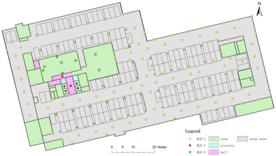
Figure 3.
Physical area division.
Virtual Area
When the physical area is large or has many beacons, directly positioning using all beacons in the area is not beneficial. It is necessary to further divide the large physical area into cell areas. If there are more than two beacons in the physical area, the algorithm will try to divide the area. Because there is no actual physical barrier, the further divided area is called the virtual area. The final division result is obtained through the virtual area division rule. Similar to the physical area, each virtual area corresponds to a set of optimal reference beacons, whose deployment structure and density are different.
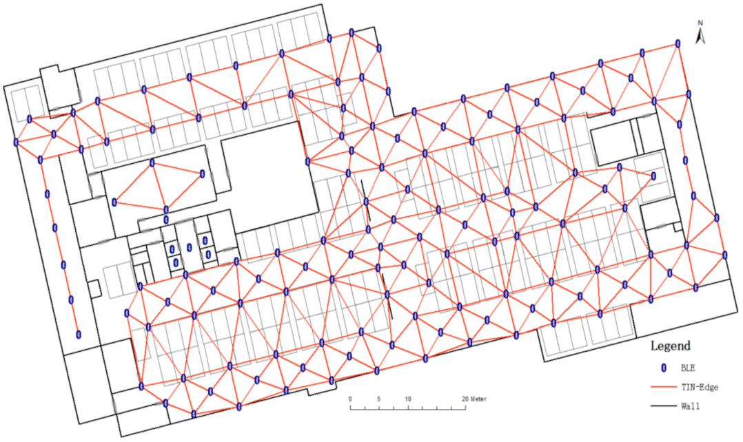
In indoor positioning, triangle-distributed beacons are often selected for positioning [22]. Based on the position of beacons, this study uses the triangulated irregular network (TIN) algorithm [38] to segregate beacons into spatially related triangles. The TIN algorithm prioritizes the characteristic of constructing an acute triangle, so that the closest beacons in space are connected, thereby achieving a more reasonable triangulation of the entire area. Figure 4 shows the result of the TIN algorithm; the two beacons are connected by a red line, which is called TIN-Edge in the present paper, indicating that there is an association between the two beacons. In particular, the TIN algorithm is only applicable when there are more than 3 beacons in the area. When the number of beacons is not more than 3, the connecting line between the beacons is TIN-Edge.
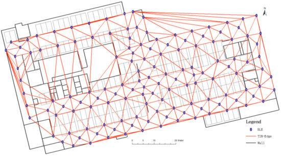
Figure 4.
Connection relationship between beacons generated by TIN.
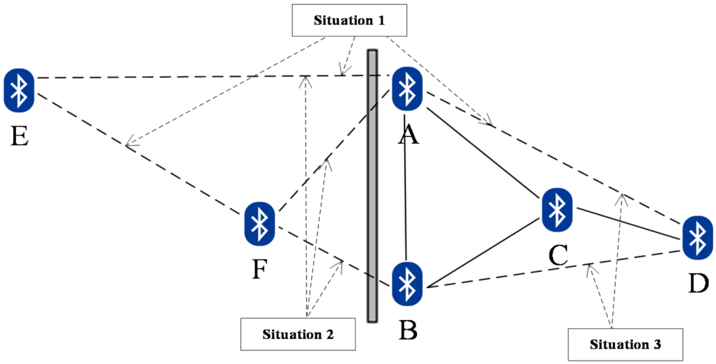
When directly using the TIN algorithm to establish the spatial connection relationship between the beacons, the actual environment was not considered. As shown in Figure 4, there are unreasonable situations such as the connection through the wall, long-distance, and multiple connections edge close to overlapping. Unreasonable connection conditions must be processed in conjunction with the map information. Three unreasonable situations are displayed and analyzed in detail, as shown in Figure 5.

Figure 5.
Three types of unreasonable spatial connections.
Situation 1: long distance. The RSSI and availability decreased as the distance increased. When a certain distance threshold is exceeded, the correlation between the two beacons is extremely weak. In this study, a threshold of 20 m was selected to eliminate excessively long connected edges.
Situation 2: connection through the wall. There is no connection relationship between the two beacons completely blocked by the wall, and the connecting edge through the wall can be eliminated by using map information.
Situation 3: multiple connected edges are close to overlapping. The beacon layout is close to linear; that is, there is a triangle with a large obtuse angle in the beacon connection. In this study, the obtuse angle threshold was 135° to eliminate the bottom edge of the triangle.
The above three situations may exist simultaneously in some scenarios. After removing the connecting edges of the above three cases, the spatial connection between the beacons is obtained, as shown in Figure 6. To facilitate the unified management of the cell area, TIN-Edge is also used to represent the beacons that have a connection relationship in the physical area.

Figure 6.
Virtual area division.
The beacons were connected by TIN-Edge, and the final spatial virtual area was constructed with TIN-edge as the center edge of the area. Depending on location, the optimal combination of beacons can be linear, triangular, quadrilateral, etc. The details are presented in the next section.
3.2.2. Optimal Combination of Beacons
For a spatial physical area that does not need to be divided, the optimal reference beacon combination of the cell area includes all the beacons in the area. For a large space divided into multiple virtual areas, the TIN-Edge connection relationship between the beacons is used to search for the optimal reference beacon combination. The beacon relationship constructed in the previous section is expressed using “Node-TIN-Edge-Node”.
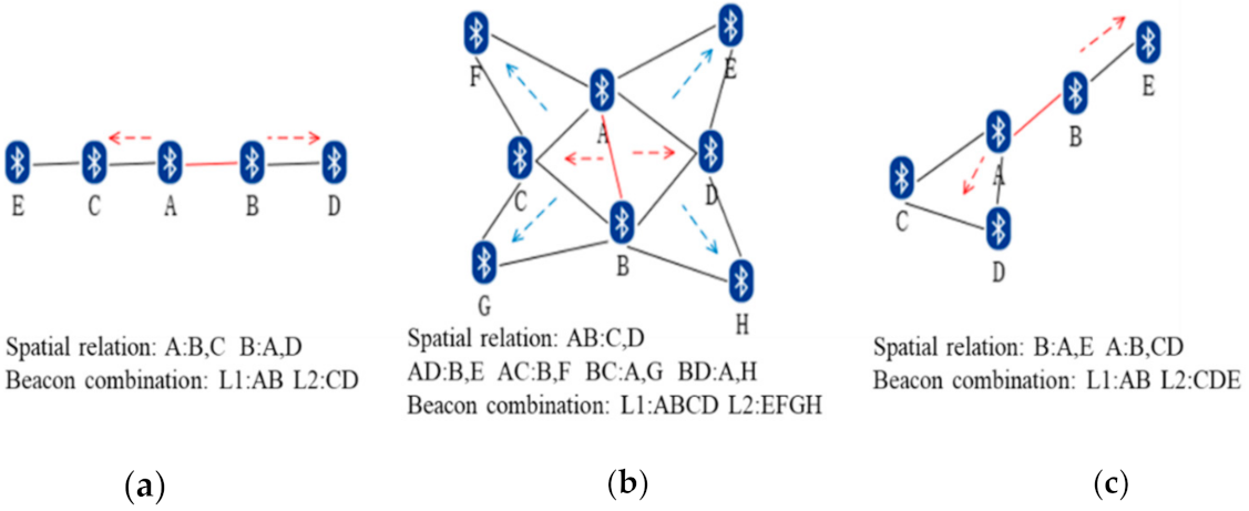
Based on the deployment of the beacon, the layout type of the reference beacon combination can be divided into four types: dots, lines, polygons, and mixed. In addition to the fact that the dot is an independent beacon node and has no correlation with other beacons, the spatial relations among the beacons differ based on layout types. Figure 7 shows the spatial relationship and optimal combination of the reference beacons of virtual area AB in different layouts. Figure 7a is a linear layout; its basic structure is line segments, and the spatial relationship is “A: B, C.” Figure 7b is a polygonal layout; the basic composition is triangles, and the spatial relationship is “AB: C, D.” Figure 7c presents a mixed layout where the basic structure includes triangles and line segments. The basic structure of the center of the area was used as the main body to construct the spatial relationship. In Figure 7c, AB is the line segment, and the spatial relationship is “A: B, C, D.” Using the spatial relationship between the beacons, the optimal reference beacon combination of the cell areas of different layouts can be obtained, and all the cell areas can be traversed to obtain the optimal reference combination. In addition, when a sub-optimal reference beacon in the cell area is required, the next-level associated beacon can also be determined based on the optimal reference beacon. L1 and L2 in each sub-picture in Figure 7 represent the optimal reference beacon combination and the suboptimal reference beacon combination of the cell area. When regional beacons are deployed linearly, the combination of L1 and L2 is used as the final reference beacon. When the beacon has a polygonal layout, L1 alone can meet the requirements of the reference beacon.

Figure 7.
The optimal reference beacon combination in the area-AB under different layouts: (a) linear layout, (b) polygonal layout, (c) mixed layout.
When stored in the library, the index of a single beacon area is the BLE point. For multiple beacon areas, the connecting edge of the BLE pair in the center of the area is used as the index of the area. For example, the edge AB in Figure 7.
3.2.3. Hierarchical Spatial Signal Coverage
The effect of the reference beacon on the cell area differs based on layouts. Different shapes and densities result in different areas having different positioning accuracies. In theory, a cell area with a reasonable density and layout usually has a better positioning accuracy [39]. In our research, according to the maximum diameter R of each cell area (the virtual area is the maximum interval between BLE beacons), the area is divided into 3 types: R < 6 m, 6 ≤ R < 12 m, and R ≥ 12 m. At the same time, the distribution of beacons in each area is as follows: polygon, line, and point. Based on the layout and density information of the beacon, the optimal reference beacons of each cell area can be scored, which is called Score_level. According to the area size and layout type, the optimal reference beacon can be divided into 9 situations. In order to simplify the calculation, this study only distinguishes situations where there is a significant difference in accuracy. Specifically, taking the score of the Polygon type as the reference standard, the score is set between 1–3, where 3 is the best and 1 is the worst. The score decreases as the area size increases. In addition, the positioning accuracy of line and point types is usually worse than that of Polygon type. Their score is also reduced by one compared to the Polygon type with the same area size. When the score is less than 1, it is set to 1. Table 1 shows the Score_level set by the algorithm in various situations. The higher the value, the higher the positioning effect of the area.

Table 1.
The score level of the reference beacon in the cell area.
Using ArcGIS buffer analysis tools, the beacon coverage of the entire area can be roughly displayed as a beacon coverage rating map, as shown in Figure 8. Areas with better positioning accuracy have better beacon density and deployment structure while areas with low ratings have poor beacon coverage. In addition, areas with high ratings primarily cover roads with high traffic frequency, which meet the positioning requirements of parking lots, and indicate that the overall beacon deployment structure is reasonable.
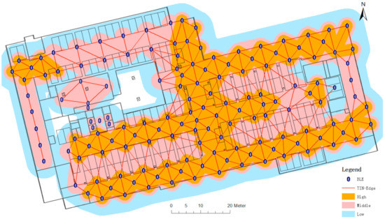
Figure 8.
Reference beacon coverage rating map of the area.
3.3. Positioning
After processing, as described in Section 3.2, the entire area is divided into multiple cell areas, and the cell area has an optimal combination of reference beacons (LO). The real-time BLE beacon sequence sorted by RSSI is referred to as LM-N where N is the number of beacons (for example, LM-4 represents the first four beacons in the sorting). The function mach_ratio (LO, LM-N) represents the ratio of the number of matching elements in the list LO and LM-N to LO. The positioning stage mainly uses LM-N and LO to recognize the cell area, and then the best reference beacons are used to select the most accurate positioning.
3.3.1. Recognize the Cell Area
A beacon with a larger RSSI usually has higher credibility [2,33,37]. Therefore, the LM-4 is used to recognize the cell area where the device is located, and this process mainly consists of two steps.
First, the area index is used to roughly find the cell area from the area library as an alternative option and construct query conditions from LM-4 by the following two methods:
- Point-index: the beacon with the largest RSSI of LM-4 is used as the point-index to the area with the single optimal beacon;
- Edge-index: two beacons of the LM-4 are used to form the edge-index of the area with multiple optimal beacons.
Second, according to the matching situation of LO and LM-4, the cell area is recognized. Based on the optimal number of reference beacons in the region, the successful matching of LO and LM-4 can be divided into the following two types:
- Single optimal beacon: the largest RSSI of LM-4 is greater than the threshold value −75, and is significantly larger than the second-largest RSSI;
- Multiple optimal beacons: match_ratio (LO, LM-4) > 0.75, That is, at least 3 beacons of LO are in LM-4, if the beacon’s number of LO is less than 4, all of them need to be matched.
3.3.2. Preferred Reference Beacons
When the area is identified, the LO of the area will be matched with scanned beacons LM-N, and then the optimal reference beacons are preferred from the LM-N. The matching results of LO and LM-N can be divided into the following three situations (the matching scores (Score_match) are shown in Table 2):
Table 2.
The Score_match of different situations.
- Good: match_ratio (LO, LM-4) = 1, LM-4 contains all the beacons of LO, indicating that the signal of these beacons is relatively stable;
- Fair: match_ratio (LO, LM-4) < 1 and match_ratio (LO, LM-8) = 1, LM-4 does not contain all the beacons of LO, and LM-8 contains all the beacons of LO, indicating that the signal of these beacons is generally stable;
- Poor: match_ratio (LO, LM-8) < 1, LM-8 does not contain all the beacons of LO, indicating that the signal of these beacons may have large noise.
Based on the optimized reference beacon, the position (P) can be calculated, and the score of P, called Score_group, can be calculated by Score_match and Score_level with Formula (1).
3.3.3. Positioning and Evaluation
Multiple sets of P and Score_group are usually generated, and we use a weighted average to obtain the final position here the weight is the ratio of each score of P to the total score, as shown in Formula (2).
The score of the average of the score of each position, as in Formula (3). The higher the score, the better the positioning accuracy.
The positioning phase following the procedure is described in Algorithm 2.
| Algorithm 2 Proposed localization algorithm with optimal beacons. |
| Input: LM-N and the library of optimal beacon combination Output: and |
|
4. Experiment and Result
4.1. Experimental Setup
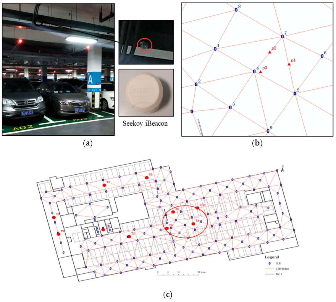
The first floor of the underground parking lot of the Wuhan Survey, Design, and Research Institute, Hubei, China, was selected as the experimental site. The actual environment and beacon deployment are shown in Figure 9a. The BLE beacon used is “Seeck Beacon”. Limited by the actual environment, the BLE is deployed on the roof or pillar. The layout structure and density of parking areas, elevator halls, and corridors are different, and the beacon interval is between 5–15 m. The experiment separately analyzed the area recognition based on the real-time BLE beacon sequence and the positioning accuracy after beacon filtering and demonstrated the dynamic positioning effect.
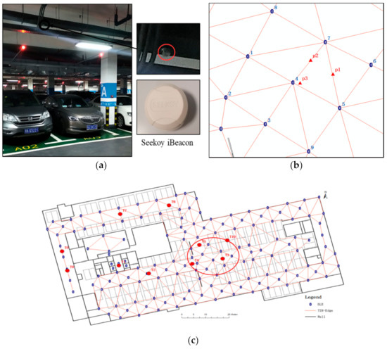
Figure 9.
Experimental scene. (a) Parking lot environment and beacon deployment. (b) Test points for virtual area recognition. (c) Test points for accuracy evaluation.
The area recognition situation is divided into two situations: physical and virtual area recognition. The physical area recognition primarily includes the room, corridor (near the beacon), elevator, and parking area, and it is judged whether the physical area identified by the algorithm is consistent with the actual situation. At the junction of physical regions, the algorithm discards this type of signal sequence when the recognition of each region is unstable, and such anomalies will be ignored in the experiment.
Virtual area recognition was primarily performed at points p1, p2, and p3 (Figure 9b). The site is shown in Figure 9b corresponds to the area in the red circle of Figure 9c in the center of the experimental area. This site has the highest beacon coverage, but problems such as crosstalk between signals are more distinct. Virtual area recognition primarily analyzes whether the cell area matched by LM-4 is area A (4-5-6-7), area B (1-4-5-7), or area C (4-9-5-7). The cell area that does not belong to the above areas is determined to be another area. If the cell area cannot be found by matching LM-4, then the match failed and is determined to be none.
The signal sequence collected at the T1–T10 positions in Figure 9 different was used to analyze the positioning accuracy of the reference beacon selected by different methods. Using four types of beacons to calculate the positioning result: the optimal reference beacon combination of the area where the known sampling points are located, the beacons with top four RSSI of beacon sequences (the general method), the beacons optimized by the APIT algorithm, and the reference beacons selected by our algorithm. The positioning results were used to evaluate the accuracy and stability of different algorithms.
The experiment uses Oppo R17 to collect BLE beacon data and collect a set of BLE beacon sequences at a frequency of 1 s. Fifty sets of signal sequences were collected at each sampling point.
4.2. Area Recognition Results
The results of the physical area recognition are shown in Table 3, where the recognition accuracy rate is 100%. The physical partition in the physical area has a significant attenuation of the RSSI, and the BLE of each physical area has a large distance, which ensures the accuracy in physical area recognition.
Table 3.
Physical area recognition results.
The results of virtual area recognition are listed in Table 4. The recognition result includes three types: matched, other, and none. “Matched” means the recognized area is a purpose area. “Other” means the recognized area is a virtual area but not a purpose area, and “none” means no virtual area is recognized. In contrast to the high accuracy rate of the physical area, the recognition of the virtual area fluctuates greatly, but it still maintains a greater probability of matching to the correct virtual area. The matching rate of P1 reached 88%, while only one set of sequences did not match; the matching rate of P2 and P3 points was lower than P1, with P3 being the lowest. The matching rate of the center of the region is higher than that of the edge of the region. When sampling at P3, the distance between the device and the beacons 1, 3, 5, and 7 are close, resulting in unstable region recognition. In addition, the area division in this article does not include areas such as areas (4-5-7-8), which will also cause the beacon sequence to be available but remain unmatched. Owing to the large overlap between virtual areas, there is a high probability that the device is located in the center of the virtual area. In general, virtual area recognition has a higher matching rate, meeting positioning requirements.
Table 4.
Virtual area recognition results.
4.3. Preferred Beacons and Positioning
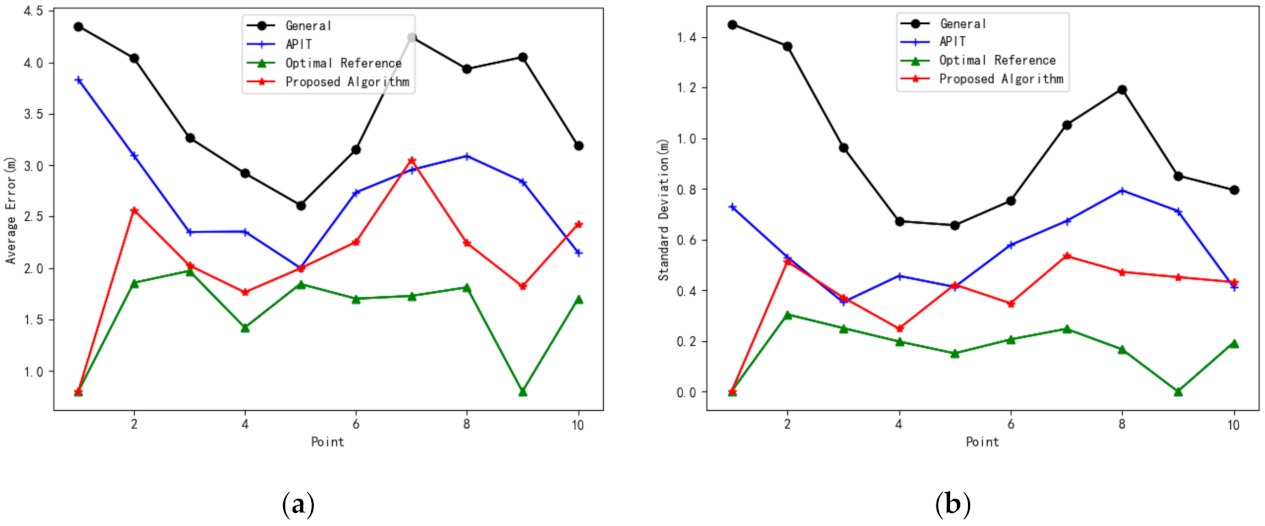
The distributions of the average error and standard deviation of the positions calculated using different methods at sampling points T1–T10 are shown in Figure 10. When the general method is used for direct positioning, the error, and standard deviation are large, and the fluctuation of the signal causes the overall positioning to be poor. The accuracy is relatively higher only in the center of the area (T3, T4, and T5). However, using the regional optimal reference beacon combination to select the beacon positioning provides the best positioning accuracy and stability, indicating the significance of accurately selecting the reference beacon for positioning accuracy. Compared with the APIT algorithm, our algorithm performs better and is closer to the optimal reference, especially when the nearest reference beacon layout does not meet the triangular structure, such as T0, T8, T9, etc. Furthermore, our algorithm considers the positioning value of the beacon while selecting the reference beacon. By determining the positioning value of the beacon sequence, our method can identify and eliminate the beacon sequence with large fluctuations, thereby ensuring positioning accuracy.
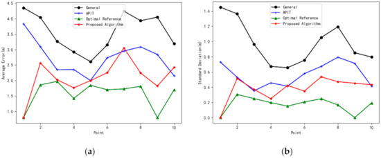
Figure 10.
Average error and standard deviation of different methods. (a) Average error. (b) Standard deviation of error.
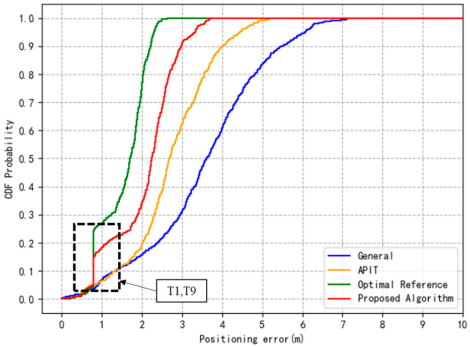
We further analyzed the overall positioning errors of the different methods at the T1-T10 test points. Figure 11 is the distribution histogram of the positioning error, Figure 12 is the cumulative distribution plot of the positioning error, and Table 5 is the statistical value of the average positioning error and standard deviation of each method. The analysis results show that the optimal reference method has significantly better positioning accuracy, and more than 80% of the positioning errors are within 2 m. It shows the superiority of positioning with the best reference beacons. Our algorithm and APIT algorithm are more accurate than the general method, and our algorithm is closer to the optimal reference than APIT. These results verify the effectiveness of our algorithm in the selection of reference beacons. Finally, the average positioning error of our algorithm in the experiment was 2.09 m.
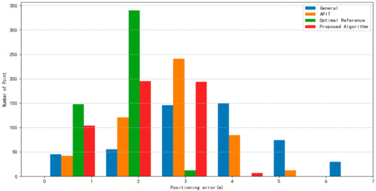
Figure 11.
Histogram plot of the positioning error.
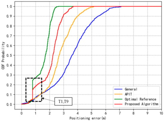
Figure 12.
The cumulative distribution function of the positioning error. The jump in the position of the black frame is caused by the test results of T1 and T9.
Table 5.
Statistical result of different methods.
4.4. Dynamic Positioning Case
The tester holds the smartphone and travels from point S to point E according to the green route in Figure 11, and the positioning result output of our algorithm is also shown in the figure. The result is displayed in different colors according to the score of the location (high, medium, and low levels). Successful output result indicates that the beacon sequence meets the algorithm-filter conditions. Figure 11 shows that the high-level points are mostly located in the center of the cell area, which is consistent with the conclusion of Section 4.2; thus, the central area has better signal coverage. The middle-level points are primarily detected along the direction of travel and also have good performance. The low-level points deviate slightly from the route.
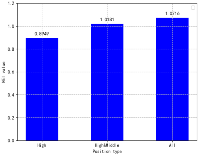
We evaluated the navigated paths using a navigation efficiency index (NEI) based on [42]. The closer the NEI is to 1, the closer it is to the true trajectory. We divided navigation paths into three cases to calculate NEI (Figure 14): high-scoring positions (High), high and middle scoring positions (High&Middle), and all the positions (All). Figure 13 and Figure 14 show that the best performance is in the High&Middle case, and the NEI value is 1.0181. Although high-scoring positions have high accuracy, too many missing points lead to missing trajectories and a low NEI value. However, adding a low-scoring position results in a large NEI due to its positioning error. In actual positioning, the positioning results can be reasonably applied according to the score guidance.
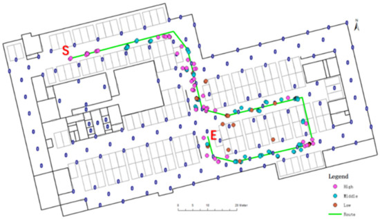
Figure 13.
A Case of dynamic positioning.

Figure 14.
Navigation efficiency index (NEI) versus position type.
5. Discussion
The map information-assisted BLE positioning algorithm proposed in this paper verifies that by selecting good BLE sequences for positioning and discarding poor ones, the accuracy of positioning can be effectively guaranteed. The real-time BLE sequence is relatively disrupted when the RSSI is affected by the environment, but when the BLE sequence is highly available, the RSSI is consistent with the actual distance.
By dividing the positioning area into multiple cell areas for analysis, the positioning algorithm and optimal reference beacon can be determined by area, which is more suitable for actual needs. For example, different areas require positioning with different accuracies, and beacons are deployed in different situations, such as single-point or multi-point deployment. In addition, in a multi-source scene where there are other positioning sources such as audio and light, the use of map information to assist area division can assist collaborative management of different sources in the multi-source scene, while enabling different positioning technologies in different areas.
However, there are still some limitations in this study. First of all, cell area recognition and reference beacon selection rely on the real-time signal sequence. If the signal contains large noise jitter, this algorithm will easily fail. Second, this study improves positioning by optimizing reference beacons without directly optimizing RSSI and positioning solution algorithms. In a real-world application, it must be used in conjunction with related algorithms. Finally, our algorithm is based on distance-based positioning. As fingerprint algorithms usually have better accuracy, the applicability of the algorithm to fingerprint positioning requires further research.
6. Conclusions
This paper proposes an indoor positioning algorithm assisted by map information in a complex beacon deployment environment. Based on the constraints of map information on beacons, the algorithm aggregates independent beacons into optimal reference beacon combinations with the cell area as the center. Then, the optimal reference beacon combination is used to select the reference beacons from the real-time beacon sequence to achieve accurate positioning. Experiments in an actual parking lot environment show that the algorithm can accurately model complex beacon deployments and can significantly improve the accuracy of positioning. However, this algorithm mainly improves the selection of reference beacons, and it needs to be combined with related algorithms to achieve accurate positioning.
Author Contributions
Wuping Liu performed the research, analyzed the data, and wrote the paper. Xinyan Zhu co-designed the research and extensively updated the paper. Wei Guo co-designed the research. All authors have read and agreed to the published version of the manuscript.
Funding
This research was funded by the National Key R&D Program of China, grant number 2016YFB0502200 and 2016YFB0502203.
Conflicts of Interest
The authors declare no conflict of interest.
References
- Liu, J.; Chen, R.; Pei, L.; Guinness, R.; Kuusniemi, H. A hybrid smartphone indoor positioning solution for mobile LBS. Sensors 2012, 12, 17208–17233. [Google Scholar] [CrossRef]
- Subedi, S.; Pyun, J.Y. A survey of smartphone-based indoor positioning system using RF-based wireless technologies. Sensors 2020, 20, 7230. [Google Scholar] [CrossRef] [PubMed]
- Davidson, P.; Piché, R. A survey of selected indoor positioning methods for smartphones. IEEE Commun. Surv. Tutor. 2016, 19, 1347–1370. [Google Scholar] [CrossRef]
- Xiao, J.; Zhou, Z.; Yi, Y.; Ni, L.M. A survey on wireless indoor localization from the device perspective. ACM Comput. Surv. 2016, 49, 1–31. [Google Scholar] [CrossRef]
- Wang, S.S. A BLE-based pedestrian navigation system for car searching in indoor parking garages. Sensors 2018, 18, 1442. [Google Scholar] [CrossRef]
- Stavrou, V.; Bardaki, C.; Papakyriakopoulos, D.; Pramatari, K. An ensemble filter for indoor positioning in a retail store using Bluetooth low energy beacons. Sensors 2019, 19, 4550. [Google Scholar] [CrossRef] [PubMed] [Green Version]
- Kunhoth, J.; Karkar, A.G.; Al-Maadeed, S.; Al-Ali, A. Indoor positioning and wayfinding systems: A survey. Hum. Centric Comput. Inf. Sci. 2020, 10, 1–41. [Google Scholar] [CrossRef]
- Palumbo, F.; Barsocchi, P.; Chessa, S.; Augusto, J.C. A stigmergic approach to indoor localization using Bluetooth low energy beacons. In Proceedings of the 12th IEEE International Conference on Advanced Video and Signal Based Surveillance (AVSS), Karlsruhe, Germany, 25–28 August 2015; IEEE Publications: Piscataway, NJ, USA, 2015; Volume 2015, pp. 1–6. [Google Scholar]
- Rida, M.E.; Liu, F.; Jadi, Y.; Algawhari, A.A.A.; Askourih, A. Indoor location position based on Bluetooth signal strength. In Proceedings of the 2nd International Conference on Information Science and Control Engineering, Shanghai, China, 24–26 April 2015; IEEE Publications: Piscataway, NJ, USA, 2015; Volume 2015, pp. 769–773. [Google Scholar]
- Zhu, J.; Luo, H.; Chen, Z.; Li, Z. RSSI based Bluetooth low energy indoor positioning. In Proceedings of the International Conference on Indoor Positioning and Indoor Navigation (IPIN), Busan, Korea, 27–30 October 2014; IEEE Publications: Piscataway, NJ, USA, 2014; Volume 2014, pp. 526–533. [Google Scholar]
- Klepal, M.; Beauregard, S. A backtracking particle filter for fusing building plans with PDR displacement estimates. In Proceedings of the 5th Workshop on Positioning, Navigation and Communication, Hannover, Germany, 27 March 2008; IEEE Publications: Piscataway, NJ, USA, 2008; Volume 2008, pp. 207–212. [Google Scholar]
- Davidson, P.; Collin, J.; Takala, J. Map-aided autonomous pedestrian navigation system. In Proceedings of the 18th International Conference Integrated Navigation Systems, Saint Petersburg, Russia, 30 May–1 June 2011; pp. 314–318. [Google Scholar]
- Nurminen, H.; Ristimäki, A.; Ali-Löytty, S.; Piché, R. Particle filter and smoother for indoor localization. In Proceedings of the International Conference on Indoor Positioning and Indoor Navigation, Montbeliard, France, 28–31 October 2013; IEEE Publications: Piscataway, NJ, USA, 2013; pp. 1–10. [Google Scholar]
- Abdulrahim, K.; Hide, C.; Moore, T.; Hill, C. Integrating low cost IMU with building heading in indoor pedestrian navigation. JGPS 2011, 10, 30–38. [Google Scholar] [CrossRef] [Green Version]
- Davidson, P.; Kirkko-Jaakkola, M.; Collin, J.; Takala, J. Navigation algorithm combining building plans with autonomous sensor data. Gyroscopy Navig. 2015, 6, 188–196. [Google Scholar] [CrossRef]
- Gilliéron, P.Y.; Büchel, D.; Spassov, I.; Merminod, B. Indoor navigation performance analysis. In Proceedings of the 8th European Navigation Conference GNSS, Rotterdam, The Netherlands, 17–19 May 2004. [Google Scholar]
- Koivisto, M.; Nurminen, H.; Ali-Loytty, S.; Piché, R. Graph-based map matching for indoor positioning. In Proceedings of the 10th International Conference on Information, Communications and Signal Processing (ICICS), Singapore, 2–4 December 2015; IEEE Publications: Piscataway, NJ, USA, 2015; Volume 2015, pp. 1–5. [Google Scholar]
- Yamamoto, D.; Tanaka, R.; Kajioka, S.; Matsuo, H.; Takahashi, N. Global map matching using BLE beacons for indoor route and stay estimation. In Proceedings of the 26th ACM SIGSPATIAL International Conference on Advances in Geographic Information Systems, Seattle, DC, USA, 6–9 November 2018; pp. 309–318. [Google Scholar]
- Aomumpai, S.; Prommak, C. On the impact of reference node placement in wireless indoor positioning systems. Int. J. Electr. Comput. Eng. 2011, 5, 1704–1708. [Google Scholar]
- Orujov, F.; Maskeliūnas, R.; Damaševičius, R.; Wei, W.; Li, Y. Smartphone based intelligent indoor positioning using fuzzy logic. Future Gener. Comput. Syst. 2018, 89, 335–348. [Google Scholar] [CrossRef]
- Obreja, S.G.; Vulpe, A. Evaluation of an indoor localization solution based on Bluetooth low energy beacons. In Proceedings of the 13th International Conference on Communications (COMM), Bucharest, Romania, 18–20 June 2020; IEEE Publications: Piscataway, NJ, USA, 2020; Volume 2020, pp. 227–231. [Google Scholar]
- Wang, Y.; Yang, X.; Zhao, Y.; Liu, Y.; Cuthbert, L. Bluetooth positioning using RSSI and triangulation methods. In Proceedings of the 10th Consumer Communications and Networking Conference (CCNC), Las Vegas, NV, USA, 11–14 January 2013; IEEE Publications: Piscataway, NJ, USA, 2013; Volume 2013, pp. 837–842. [Google Scholar]
- Kaczmarek, M.; Ruminski, J.; Bujnowski, A. Accuracy analysis of the RSSI BLE SensorTag signal for indoor localization purposes fed. In Proceedings of the Conference on Computer Science and Information Systems (FedCSIS), Gdansk, Poland, 11–14 September 2016; IEEE Publications: Piscataway, NJ, USA, 2016; Volume 2016, pp. 1413–1416. [Google Scholar]
- Zhang, K.; Zhang, Y.; Wan, S. Research of RSSI indoor ranging algorithm based on Gaussian-Kalman linear filtering. In Proceedings of the IEEE Advanced Information Management, Communicates, Electronic and Automation Control Conference (IMCEC), Xi’an, China, 3–5 October 2016; IEEE Publications: Piscataway, NJ, USA, 2016; Volume 2016, pp. 1628–1632. [Google Scholar]
- Mackey, A.; Spachos, P.; Song, L.; Plataniotis, K.N. Improving BLE beacon proximity estimation accuracy through Bayesian filtering. IEEE Internet Things J. 2020, 7, 3160–3169. [Google Scholar] [CrossRef] [Green Version]
- Lam, C.H.; Ng, P.C.; She, J. Improved distance estimation with BLE beacon using Kalman filter and SVM. In Proceedings of the IEEE International Conference on Communications (ICC), Kansas City, MO, USA, 20–24 May 2018; IEEE Publications: Piscataway, NJ, USA, 2018; Volume 2018, pp. 1–6. [Google Scholar]
- Rajagopal, N.; Chayapathy, S.; Sinopoli, B.; Rowe, A. Beacon placement for range-based indoor localization. In Proceedings of the 2016 International Conference on Indoor Positioning and Indoor Navigation (IPIN), Alcala de Henares, Spain, 4–7 October 2016; IEEE: Piscataway, NJ, USA, 2016; pp. 1–8. [Google Scholar]
- Bulusu, N.; Heidemann, J.; Estrin, D. Adaptive beacon placement. In Proceedings of the 21st International Conference on Distributed Computing Systems, Mesa, AZ, USA, 16–19 April 2001; IEEE Publications: Piscataway, NJ, USA, 2001; pp. 489–498. [Google Scholar]
- Ng, P.C.; She, J.; Park, S. High resolution beacon-based proximity detection for dense deployment. IEEE Trans. Mob. Comput. 2017, 17, 1369–1382. [Google Scholar] [CrossRef]
- Juri, A.A.; Arslan, T.; Wang, F. Obstruction-aware Bluetooth low energy indoor positioning. In Proceedings of the 29th International Technical Meeting of the Satellite Division of the Institute of Navigation (ION GNSS+ 2016), Oregon, Portland, 12–16 September 2016; pp. 2254–2261. [Google Scholar]
- Tomic, S.; Beko, M.; Dinis, R.; Dimic, G.; Tuba, M. Distributed RSS-based localization in wireless sensor networks with node selection mechanism. In Doctoral Conference on Computing, Electrical and Industrial Systems; Springer: Cham, Switzerland, 2015; pp. 204–214. [Google Scholar]
- He, T.; Huang, C.; Blum, B.M.; Stankovic, J.A. Range-free localization schemes for large scale sensor networks. In Proceedings of the 9th Annual International Conference on Mobile Computing and Networking, San Diego, CA, USA, 14–19 September 2003; pp. 81–95. [Google Scholar]
- Al-Madani, B.; Orujov, F.; Maskeliūnas, R.; Wei, W.; Li, Y. Fuzzy logic type-2 based wireless indoor localization system for navigation of visually impaired people in buildings. Sensors 2019, 19, 2114. [Google Scholar] [CrossRef] [PubMed] [Green Version]
- Lee, K.; Nam, Y.; Min, S.D. An indoor localization solution using Bluetooth RSSI and multiple sensors on a smartphone. Multimedia Tool. Appl. 2018, 77, 12635–12654. [Google Scholar] [CrossRef]
- Liu, L.; Li, B.; Yang, L.; Liu, T. Real-time indoor positioning approach using iBeacons and smartphone sensors. Appl. Sci. 2003, 10, 2003. [Google Scholar] [CrossRef] [Green Version]
- Li, Y.S.; Ning, F.S. Low-cost indoor positioning application based on map assistance and mobile phone sensors. Sensors 2018, 18, 4285. [Google Scholar] [CrossRef] [PubMed] [Green Version]
- Wang, W.; Marelli, D.; Fu, M. Dynamic Indoor Localization Using Maximum Likelihood Particle Filtering. Sensors 2021, 21, 1090. [Google Scholar] [CrossRef]
- Bhargava, N.; Bhargava, R.; Tanwar, P.S. Triangulated irregular network model from mass points. Int. J. Adv. Comput. Res. 2013, 3, 172. [Google Scholar]
- Sadowski, S.; Spachos, P. Optimization of BLE beacon density for RSSI-based indoor localization. In Proceedings of the IEEE International Conference on Communications Workshops (ICC Workshops), Shanghai, China, 20–24 May 2019; IEEE Publications: Piscataway, NJ, USA, 2019; Volume 2019, pp. 1–6. [Google Scholar]
- Liang, S.C.; Liao, L.H.; Lee, Y.C. Localization algorithm based on improved weighted centroid in wireless sensor networks. J. Netw. 2014, 9, 183. [Google Scholar] [CrossRef]
- Chuku, N.; Pal, A.; Nasipuri, A. An RSSI based localization scheme for wireless sensor networks to mitigate shadowing effects. In Proceedings of the IEEE Southeastcon, Jacksonville, FL, USA, 4–7 April 2013; IEEE Publications: Piscataway, NJ, USA, 2013; Volume 2013, pp. 1–6. [Google Scholar]
- Ganz, A.; Schafer, J.; Gandhi, S.; Puleo, E.; Wilson, C.; Robertson, M. PERCEPT indoor navigation system for the blind and visually impaired: Architecture and experimentation. Int. J. Telemed. Appl. 2012, 2012, 19. [Google Scholar] [CrossRef] [PubMed]


Publisher’s Note: MDPI stays neutral with regard to jurisdictional claims in published maps and institutional affiliations. |
© 2021 by the authors. Licensee MDPI, Basel, Switzerland. This article is an open access article distributed under the terms and conditions of the Creative Commons Attribution (CC BY) license (https://creativecommons.org/licenses/by/4.0/).