Indoor Emergency Path Planning Based on the Q-Learning Optimization Algorithm

Abstract

The internal structure of buildings is becoming increasingly complex. Providing a scientific and reasonable evacuation route for trapped persons in a complex indoor environment is important for reducing casualties and property losses. In emergency and disaster relief environments, indoor path planning has great uncertainty and higher safety requirements. Q-learning is a value-based reinforcement learning algorithm that can complete path planning tasks through autonomous learning without establishing mathematical models and environmental maps. Therefore, we propose an indoor emergency path planning method based on the Q-learning optimization algorithm. First, a grid environment model is established. The discount rate of the exploration factor is used to optimize the Q-learning algorithm, and the exploration factor in the ε-greedy strategy is dynamically adjusted before selecting random actions to accelerate the convergence of the Q-learning algorithm in a large-scale grid environment. An indoor emergency path planning experiment based on the Q-learning optimization algorithm was carried out using simulated data and real indoor environment data. The proposed Q-learning optimization algorithm basically converges after 500 iterative learning rounds, which is nearly 2000 rounds higher than the convergence rate of the Q-learning algorithm. The SASRA algorithm has no obvious convergence trend in 5000 iterations of learning. The results show that the proposed Q-learning optimization algorithm is superior to the SARSA algorithm and the classic Q-learning algorithm in terms of solving time and convergence speed when planning the shortest path in a grid environment. The convergence speed of the proposed Q- learning optimization algorithm is approximately five times faster than that of the classic Q- learning algorithm. The proposed Q-learning optimization algorithm in the grid environment can successfully plan the shortest path to avoid obstacle areas in a short time.

1. Introduction

In recent years, with the advancement of urbanization, the internal structure of urban buildings has become more complex and variable. The hidden danger of urban disasters is partially aggravated by the highly concentrated urban population and resources [1]. Urban disasters are complex and occur suddenly, and the intricate spatial structure of urban buildings significantly affects emergency rescue [2,3]. From the summary and analysis of many emergency cases, the probability of casualties caused by improper evacuation is shown to be increasing [3]. In actual disaster scenarios, most casualties are caused by a lack of timely and effective rescue. It is of great significance to scientifically and reasonably analyze the internal structure of the indoor environment, quickly determine the dynamic changes of the evacuees’ positions, and realize the rapid and safe evacuation and rescue of personnel in emergencies [4]. Considering the increasing frequency of disaster events and increasing demand for disaster prevention and mitigation, new technologies and theoretical knowledge such as deep learning and reinforcement learning should be applied scientifically and rationally to design reasonable emergency evacuation path planning according to the internal environment of the disaster area. Reasonable path planning can arrange the orderly transfer of the affected people and effectively shorten the evacuation time, which is one of the current leading issues of social public security urgently being solved and a research hotspot of relevant scholars at home and abroad [5].

Since the mid-twentieth century, many scholars have carried out extensive research on path planning in emergency rescue situations [6]. Around the 1960s, with the rapid development of computer science, various path planning algorithms endlessly emerged. The path planning algorithm has developed from the original traditional algorithm and graphics algorithm to a bionic search algorithm and artificial intelligence algorithm. These path planning algorithms have different characteristics in the development stages, and the scope of their application and scenarios are different. In practical applications, the problem to be solved and the characteristics of the algorithm are considered comprehensively, and an appropriate path planning algorithm is selected [7]. In recent years, with the development of intelligence science and the boom in artificial intelligence, artificial intelligence path planning technology has rapidly become the focus of research by experts and scholars, while reinforcement learning algorithms have received more attention [8]. Reinforcement learning can be used to solve obstacle avoidance, path planning, and other problems collaboratively without establishing mathematical models and environmental maps for path planning problems. Lu et al. [9] proposed a neural network based on a reinforcement learning algorithm, conducted local path planning experiments, and obtained path planning results in an environment without prior knowledge. He et al. [10] proposed a combination of Q-learning and fuzzy logic technology to achieve self-learning of mobile robots and path planning in uncertain environments. Hyansu et al. [11] proposed a combination of deep Q-learning and CNN so that the robot can move flexibly and efficiently in various environments. Maw et al. [12] proposed a hybrid path planning algorithm that uses the path planning algorithm of the time graph for global planning and deep reinforcement learning for local planning so that unmanned aerial vehicles (UAVs) can avoid collisions in real time. Junior et al. [13] proposed a Q-learning algorithm based on a reward matrix to meet the route planning requirements of marine robots. Due to its characteristics, reinforcement learning has been widely used for path planning, especially for local path planning in unknown environments. However, reinforcement learning has the inherent problem of balancing exploration and utilization. In reinforcement learning, the environment is unknown to the agent. Excessive exploration of the environment by the agent will reduce the efficiency of the solution, and excessive use of the environment will cause the agent to miss the optimal solution. Therefore, the balance of exploration and utilization is an important research topic in reinforcement learning. Jaradat et al. [14] applied the Q-learning algorithm for the navigation of mobile robots in a dynamic environment and controlled the size of the Q value table to increase the speed of the navigation algorithm. Wang et al. [15] combined the two algorithms based on the better final performance of the Q-learning algorithm and the faster convergence of the SARSA (State-Action-Reward-State-Action) algorithm and proposed a reverse Q-learning algorithm, which improved the learning rate and algorithm performance. Zeng et al. [16] proposed a supervised reinforcement learning algorithm based on nominal control and introduced supervision into the Q-learning algorithm, thereby accelerating the algorithm convergence. Fang et al. [17] proposed a heuristic reinforcement learning algorithm based on state backtracking, which improved the action selection strategy of reinforcement learning, removed meaningless exploration steps, and greatly improved the learning rate. Song et al. [18] established a mapping relationship between the existing or learned environmental information and the initial value of the Q value table and accelerated learning by adjusting the initial value in the Q value table [19,20]. Zhang et al. [21] used an enhanced exploration strategy to replace ε-greedy in the traditional Q-learning algorithm and proposed a self-adaptive reinforcement exploration Q-learning (SARE-Q) algorithm to improve the exploration efficiency. Zhuang et al. [22] proposed a multi-destination global path planning algorithm based on the optimal obstacle value. According to the Q-learning algorithm, the parameters of the reward function were optimized to improve the path planning efficiency of a mobile robot driving in multiple destinations. Soong et al. [23] introduced the concept of partially guided Q-learning and initialized the Q-table through the flower pollination algorithm (FPA) to accelerate the convergence of Q-learning. ε- greedy strategy is a common method to solve the problem of balance between exploration and utilization. On the basis of Q-learning combined with ε-greedy, Li C et al. [24] proposed a parameter dynamic adjustment strategy and trial-and-error action deletion mechanism, which not only realized the balance between adaptive adjustment and utilization in the learning process, but also improved the exploration efficiency of the agent. Yang T et al. [25] proposed an ε-greedy strategy that adaptively adjusts the exploration factor, which improves the quality of the strategy learned by the agent and better balances exploration and utilization.

The abovementioned scholars have made helpful advances to improve the efficiency of reinforcement learning algorithms. However, in large and complex emergency environments, it is difficult for reinforcement learning algorithms to achieve the desired results. Since there is no prior learning knowledge, the agent can only randomly select actions for blind search, which leads to the disadvantages of low learning efficiency and slow convergence speed in the complex environment. Therefore, this paper proposes a path planning algorithm based on a grid environment and optimizes the Q-learning algorithm by introducing the calculation of the exploratory factor discount rate. The discount rate of the exploration factor is calculated before the agent selects random actions to solve the problem of blind searching in the learning process. The main contributions are summarized as follows:

• Aimed at the path planning problem of indoor complex environments in disaster scenarios, a grid environment model is established, and the Q-learning algorithm is adopted to implement the path planning problem of the grid environment.
• Aimed at the problems of slow convergence speed and low accuracy of the Q-learning algorithm in a large-scale grid environment, the exploration factor in the ε-greedy strategy is dynamically adjusted, and the discount rate variable of the exploration factor is introduced. Before random actions are selected, the discount rate of the exploration factor is calculated to optimize the Q-learning algorithm in the grid environment.
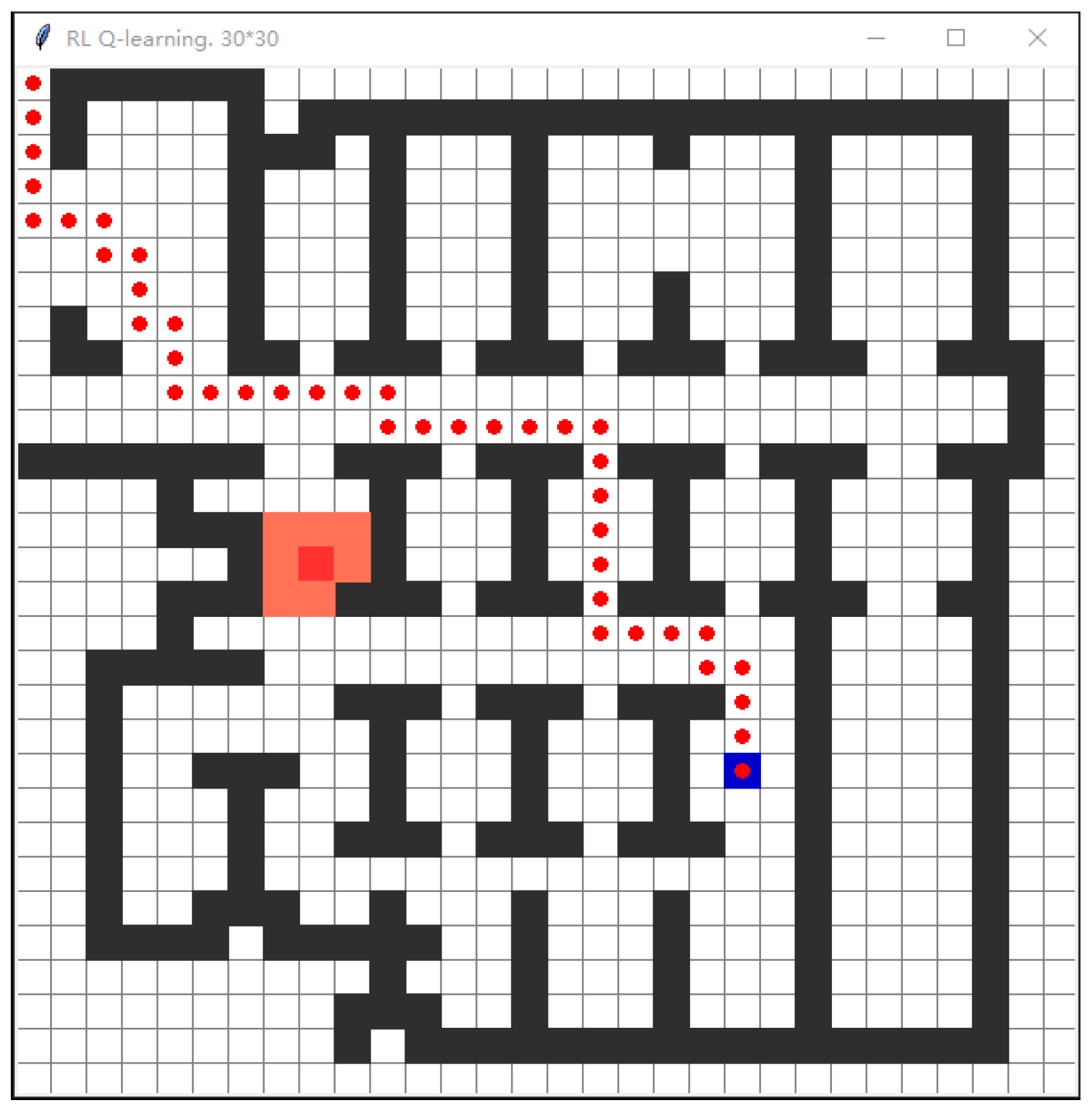
• An indoor emergency path planning experiment based on the Q-learning optimization algorithm is carried out using simulated data and real indoor environment data of an office building. The results show that the Q-learning optimization algorithm is better than both the SARSA algorithm and the Q-learning algorithm in terms of solving time and convergence when planning the shortest path in a grid environment. The Q-learning optimization algorithm has a convergence speed that is approximately five times faster than that of the classic Q-learning algorithm. In the grid environment, the Q-learning optimization algorithm can successfully plan the shortest path to avoid obstacles in a short time.

The rest of the paper is organized as below: Section 1 introduces indoor emergency path planning based on the proposed Q-learning optimization algorithm in grid environment. Section 2 introduces the algorithm simulation experiment and the experiment of indoor emergency path planning based on the proposed Q-learning optimization algorithm. Section 3 concludes this paper and shows the interesting future work related to our studies.

2. Indoor Emergency Path Planning Method

Based on the advantage that Q-learning in reinforcement learning can solve obstacle avoidance, path planning, and other problems in a unified way without establishing a mathematical model and environment map, this paper proposes an indoor emergency path planning method based on Q-learning. First, the grid graph method is used to model the grid environment. Next, the path planning strategy of the Q-learning algorithm is designed based on the grid environment, and then the Q-learning algorithm based on the grid environment is optimized by the dynamic adjustment of exploration factors.

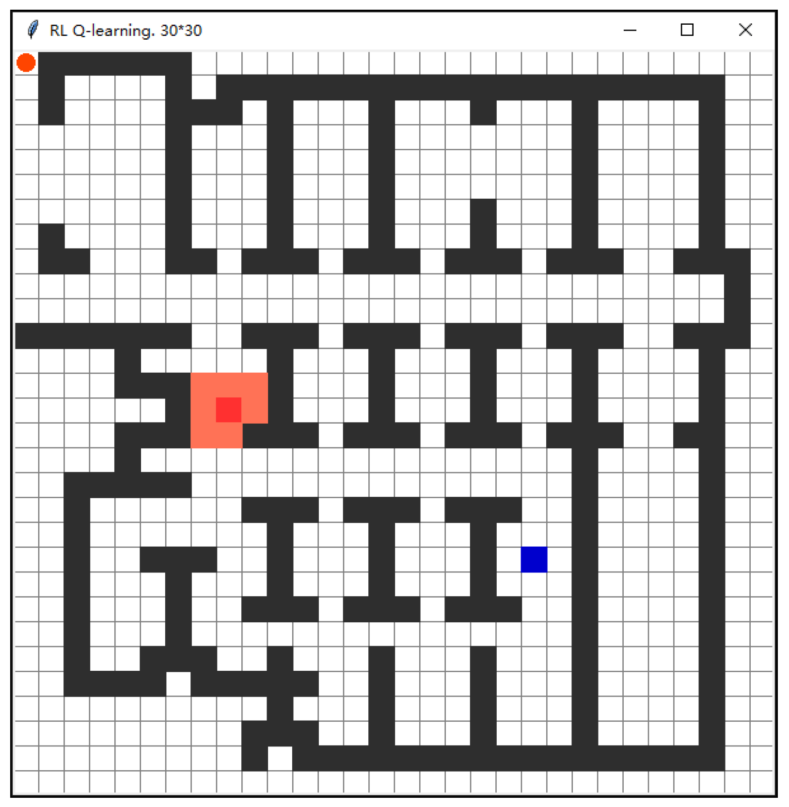
2.1. Grid Environment Modeling

The environmental modeling problem refers to how to effectively express environmental information through specific models. Environmental modeling is necessary to perform before path planning. Before global path planning, it is necessary to model the environment where the emergency personnel are located and obtain complex environmental information. This allows the emergency personnel to know the location of fixed obstacles in the environment in advance, which is an essential step in path planning.

Common methods used in environmental modeling include the viewable method [26], cell tree method [27], link graph method [28], grid graph method [29], etc. The advantages and disadvantages of these four methods are shown in

Table 1. Comparison of advantages and disadvantages of the four modeling methods.

Method	Advantages	Disadvantages
Viewable method	The algorithm principle is simple and easy to implement	Inefficient and inflexible
Cell tree method	Close attention to details	Not suitable for environments with small volume and large number of obstacles
Link graph method	Flexible, and the model does not need to be rebuilt when changing the starting and ending point	When the number of obstacles is large, the algorithm becomes complex
Grid graph method	Simple theory, easy to implement	The timeliness of the algorithm decreases as the number of grids increases

:

According to the characteristics of the emergency environment and the comparison of the advantages and disadvantages of modeling methods, this paper adopts the grid graph method for environmental modeling. The principle is to rasterize the environmental information and use various color features to represent the different environmental information. As shown in Figure 1, the black grid represents the impassable area, denoted by “1”; the white grid represents the free areas that can be accessed, denoted by “0”.

After learning the initial position and the target position, the agent explores and learns in a black-and-white grid environment to obtain the shortest obstacle avoidance path plan. The theoretical knowledge of the grid graph method is concise and easy to understand, which is convenient for program code writing and operation.

The grid graph information can be represented by a matrix. The matrix corresponding to the grid graph in Figure 1 is Equation (1):

$$D=\left[\begin{array}{cccccc}0& 0& 1& 0& 1& 0\\ 0& 1& 0& 0& 0& 1\\ 0& 0& 0& 0& 0& 0\\ 0& 0& 1& 0& 0& 0\\ 0& 0& 0& 0& 1& 0\\ 0& 1& 0& 0& 0& 0\end{array}\right]$$

(1)

2.2. Q-Learning Optimization Algorithm

Reinforcement learning is a method of machine learning, its essence is to find an optimal decision through continuous interaction with the environment [30]. The idea of reinforcement learning is as follows: The agent affects the environment by performing actions. The environment receives a new action, it will generate a new state and give reward feedback to the agent’s actions. Finally, the agent chooses the next action to perform according to the new state and reward feedback. The reinforcement learning model is shown in Figure 2.

Q-learning, proposed by Watkins in 1989, is a landmark discovery in the development of reinforcement learning. Q-learning obtains the optimal strategy by continuously estimating the state value function and optimizing the Q function [31,32]. Q-learning is different from the common time-difference method (TD) to some extent. It adopts the $Q(s,a)$ function of the state-action pair to carry out iterative calculations. In the learning process of the agent, it is necessary to check whether the corresponding behavior is reasonable in order to ensure the final result converges [33,34].

2.2.1. Q-Learning Algorithm

Q-learning is a reinforcement learning algorithm based on the finite Markov decision process, which is mainly composed of agent, state, action, and environment. The state at a certain moment is represented by $s$, and the action to be performed by the agent is represented by $a$. Q-learning initializes the function $Q(s,a)$ and state value $s$, and selects an action $a$ according to a strategy, such as ε-greedy [35], to obtain the next state $s^{\prime }$ and the immediate return $r$. Next, the Q value is updated according to the update rules [34]. When the agent reaches the destination during the movement, the algorithm completes an iteration. The agent returns to the initial node to continue the iteration cycle until the iterative learning process is complete [36,37].

In the Q-learning process, the optimal value function is determined and approximated by the optimal iterative calculation of the $Q(s,a)$ function. The update rules of the function are shown in Equations (2) and (3):

$$Q(s,a)=r+\gamma {\max }_{a^{\prime }}Q(s^{\prime },a^{\prime })$$

(2)

$$Q(s,a)=(1-\alpha )Q(s,a)+\alpha \left[r+\gamma {\max }_{a^{\prime }}Q(s^{\prime },a^{\prime })\right]$$

(3)

where $\gamma$ represents the discount factor, $\alpha$ represents the learning rate, and $a^{\prime }$ represents the next action.

The Q-learning process includes many episodes, and all episodes will repeat the following calculation process. When the agent is at time $t$:

• Observe the status $s_t$ at this time;
• Select the action $a_t$ to perform next;
• Continue to observe the next step $s_{t+1}$;
• Get immediate reward $r_t$;
• Update the $Q_{t-1}(s_t,a_t)$ value;

  $$Q(s_t,a_t)=\{\begin{array}{cc}(1-\alpha )Q_{t-1}(s_t,a_t)+\alpha \left[r_t+\gamma \underset{a^{\prime }}{\max Q_{t-1}(s_{t+1},a)}\right],& s=s_t,a=a_t\\ Q(s_t,a_t),& otherwise\end{array}$$

  (4)
• $t\leftarrow t+1$ goes to the next moment.

The Q function is represented and implemented by a lookup table and neural network.

When using a lookup table, the number of elements in the Cartesian product of $S\times A$ represents the size of the table. When the state set $S$ and the environment’s possible operation set $A$ are relatively large, a huge storage space will be occupied, and the learning efficiency will be greatly reduced. This has certain deficiencies for daily applications.

When using a neural network, $s_t=\left[s_{t1},s_{t2},\dots ,s_{tm}\right]$ is the corresponding state vector of the network input. The output results of each network correspond to the Q value of an action. Neural networks store input–output correspondence [33]. The Q function definition is shown in Equation (5):

$$Q_t^{\prime }=r_t+\gamma {\max }_{a\in A}\left\{Q\left(s_{t+1},a\right)\right\}$$

(5)

Equation (5) is effective only when the optimal strategy is obtained. In the process of the learning operation, Equation (6) is:

$$\Delta Q_i=r_t+\gamma {\max }_{a\in A}Q\left(s_{t+1},a_{t+1}\right)-Q\left(s_t,a_t\right)$$

(6)

where $Q(s_{t+1},a_{t+1})$ represents the corresponding Q value of the next state. The purpose of $\Delta Q$ is to reduce error. The weight adjustment calculation is shown in Equation (7):

$$\Delta W_t=\alpha \left[r_t+\gamma {\max }_{a\in A}Q(s_{t+1},a_{t+1})-Q(s_t,a_t)\right]$$

(7)

The specific algorithm is as follows:

• Initialize Q value;
• Select the status $s_t$ at time $t$;
• Update $Q(s,a)$;
• Select the next $a_i$ action according to the updated $Q(s_t,a_i)$;
• Perform action $a_i$, obtain the new state $s_{t+1}$ and immediate reward value $r_t$;
• Calculate $Q_t^{\prime }=r_t+\gamma {\max }_{a\in A}\left\{Q(s_{t+1},a)\right\}$;
• Adjust the weight of the Q network to minimize error $\Delta Q_i$, as shown in Equation (8):

  $$\Delta Q_i=\{\begin{array}{cc}{Q}^{\prime }-Q_i,\hfill & i=j\\ 0,\hfill & otherwise\end{array}$$

  (8)
• Go to 2.

2.2.2. Path Planning Strategy

When the agent uses the Q-learning algorithm to plan a path in an unknown obstacle environment, experience must be accumulated by continuously exploring the environment. The agent uses the ε-greedy strategy for action selection and obtains immediate rewards when performing state transitions. During each iteration, when the agent reaches the target location, the Q value table is updated. The agent position is instantly transferred to the starting point for loop iteration until the value function tends to converge, which means the learning process has finished. To improve the exploration efficiency and convergence speed of the value-added function, the agent will be given a negative reward if an obstacle is encountered during the learning process. Then, the agent can change directions to explore other positions, reduce the probability of falling into the local optimal solution, and reduce the consumption of the total number of episodes in trial-and-error learning.

1.

Action and state of agent

If the agent is regarded as a particle that does not need to consider the area, the size of the agent does not need to be taken into account when performing experimental analysis. The grid occupied by the particle is the current position of the agent, and the coordinates $(x_i,y_i)$ are used to represent the corresponding state information. In the grid environment, the agent moves one grid for every step. The agent can move in four directions: up, down, left, and right. The action space $A=\{0,1,2,3\}$ corresponds to the four directions of movement.

2.

Set the reward function

The reward function is the value feedback that the agent receives when exploring the environment. If the agent performs the optimal action, a larger reward will be obtained. If the agent performs a poor action, a smaller reward will be obtained. Actions with a high reward value will have an increased chance of being selected, while actions with a low reward value will have a decreased chance of being selected. In this section, the path planning strategy in the grid environment is to select the path along which the agent obtains the largest cumulative reward in the learning process. The specific reward function is defined by a nonlinear piecewise function, as shown in Equation (9):

$$r=\{\begin{array}{cc}1,& \mathrm{reach} \mathrm{the} \mathrm{target} \mathrm{position}\\ 0,& \mathrm{reach} \mathrm{other} \mathrm{position}\\ -1,& \mathrm{reach} \mathrm{the} \mathrm{obstacle} \mathrm{position}\end{array}$$

(9)

In the learning process, when the agent reaches the target location while exploring the environment, a reward value of $r=1$ is obtained and the training continues to the next plot. When the agent moves in the free zone, the reward value of feedback is $r=0$ When an agent encounters an obstacle area, the reward is $r=-1$.

3.

Action strategy selection

The ε-greedy algorithm is used to select the action strategy. The probability of $1-\epsilon$ is used to select the action with the maximum state action value. The probability $\epsilon$ is used to select the random action. Finally, the strategy with the largest cumulative reward value is selected. The calculation of the ε-greedy strategy is shown in Equation (10):

$$prob(a_t)=\{\begin{array}{cc}1-\epsilon ,& if a=\arg {\max }_{a_t\in A}Q(s,a_t)\\ \epsilon ,& others\end{array}$$

(10)

where prob(a(t)) represents the agent’s choice of action strategy.

4.

Q Value Table

The agent selects the action sequence with the maximum reward value as the optimal path in the final Q value table. In an $N\times N$ grid environment, $N^2$ status information indicates positions. Each position can move in four directions: up, down, left, and right, so there are $N^2\times 4$ values stored in the Q value table. Initially, all of the values in the Q value table are set to 0. When learning, check whether the state action exists in the table. If not, add the Q value to the corresponding position. If the state action exists, modify the Q value in the table.

2.2.3. Dynamic Adjustment of Exploration Factors

The Q-learning algorithm adopts the ε-greedy exploration strategy, which determines the decision the agent makes each time. $\epsilon$ is the exploration factor, which ranges from 0 to 1. As $\epsilon$ approaches 1, the agent is more inclined to explore the environment, i.e., to try random actions. However, if the agent is always inclined to explore the environment, random actions are not suitable for finding the final goal [35]. As $\epsilon$ approaches 0, the agent tends to take advantage of the external environment and choose the action with the largest action value function. In this case, the value function may not converge effectively, and the result will be influenced by the environment. Thus, the optimal solution can be easily missed and the final solution may not be obtained. The $\epsilon$ value is closely related to the agent’s exploration strategy, which determines the accuracy and efficiency of the final solution. Thus, selection of the $\epsilon$ value is vital [38].

This paper optimizes the Q-learning algorithm by dynamically adjusting the exploration factor in the ε-greedy strategy, introduces the discount rate of the exploration factor, and calculates the discount rate of the exploration factor before selecting random actions, as shown in Equation (11):

$$\epsilon (epsilon)\leftarrow \exp (-{\epsilon }_{deca{y}_{rate}}\times i)$$

(11)

where $i$ is the episode (number of iterations). When the initial value of $i$ is 0, the initial value of $\epsilon$ is 1 according to the formula, and the rate is at the maximum value. Many explorations have been conducted by randomly choosing actions and constantly training the Q function, and the agent has become increasingly confident about the estimated Q value. At the same time, with an increasing number of iterations, the proportion of the exploration factor will gradually decrease so that the agent will make more use of the external environment to improve the convergence speed when making the next selection.

2.3. Algorithm Flow

First, initialize the relevant parameters and set $i$ to 0. Before choosing a random action, the discount rate of the exploration factor is calculated. Then, perform the action according to the ε-greedy action strategy and move to the next position to obtain the corresponding state $s$ and immediate reward $r$. The Q value is updated according to the update rules of the value function calculation formula. When the training times do not meet the initial set value, the cycle is iterated. After meeting the requirements, Q values corresponding to all states are output, and the algorithm learning is finished.

A flow chart based on the Q-learning optimization algorithm in the grid environment is shown in Figure 3:

3. Experiment and Analysis

In the algorithm simulation experiment, the Q-learning algorithm, SARSA algorithm, and the proposed Q-learning optimization algorithm are used to plan the emergency path, and the experimental results are compared and analyzed. Aiming at the simulation scene, according to a real indoor environment, indoor emergency path planning analysis based on the proposed Q-learning optimization algorithm is performed.

3.1. Parameter Settings

After many experiments, the parameters of the proposed Q-learning optimization algorithm are set as follows: learning rate $\alpha =0.01$, exploration probability $\epsilon =0.9$, and discount factor $\gamma =0.9$. In the algorithm simulation experiment, the number of training episodes is set to 5000. The Q-learning algorithm and SARSA algorithm parameters are set to be consistent with the proposed Q-learning optimization algorithm parameter settings. In the simulation scene experiment, the number of training scenarios is increased to 10,000 due to the increased grid size.

3.2. Algorithm Simulation Experimental Analysis

The TD can be divided into two types: online control algorithm SARSA and offline control algorithm Q-learning. The largest difference between Q-learning and the SARSA algorithm is the method for updating the Q value. The Q-learning algorithm is bolder in the choice of actions and is more inclined to select a behavior that is not related to a strategy corresponding to the current state but a behavior that represents the maximum action value. The SARSA algorithm is more conservative in its selection and will update the Q value according to its own learning rhythm [39]. The following is based on the Q-learning algorithm, SARSA algorithm, and the proposed Q-learning optimization algorithm to determine the shortest path under the grid environment model and compare and analyze the experimental results.

3.2.1. Environmental Spatial Modeling

In this experiment, the Tkinter toolkit [40] was used to build an environmental model. In the algorithm simulation experiment, a grid environment with 20 pixels and a total number of 25 × 25 grids is constructed as an obstacle map. The agent selects and executes actions under this environmental model. The total number of grids in the environment is the number of states of the agent’s activity. As shown in Figure 4, there are a total of 625 states. The agent is represented by a red circle. The agent moves a grid on the map each time it performs an action. The initial point for this experiment is $(1,1)$, and the target point is the blue grid at the lower right corner $(21,21)$. The white grid represents the passable area, and the black grid represents the obstacle area. In Tkinter, the position of the rectangle is represented by the coordinates of two diagonal points, and the circle representing the agent is the inscribed circle of the rectangle. This has considerable convenience for representing the location. In the program, the map environment and the location of the agent can be designed by adjusting the grid coordinates. By observing the operation interface in Figure 4, the real-time position of the agent is known at each moment so that we can observe when the agent can plan the shortest path, which provides a reference for setting and adjusting the parameters.

3.2.2. Comparison and Analysis of Experimental Results

The simulation result of path planning for the agent from the starting position to the target position using the SARSA algorithm in a grid environment is shown in Figure 5a. The shortest path was 102 steps, and the longest path was 3682 steps. The simulation results of path planning using the Q-learning algorithm strategy are shown in Figure 5b. The shortest path was 42 steps, and the longest path was 1340 steps. The result of the proposed Q-learning optimization algorithm is shown in Figure 5c. The shortest path also was 42 steps, and the longest path was 1227 steps. There is little difference between the path planning results of the Q-learning algorithm and the proposed Q-learning optimization algorithm, but the results are significantly better than the results using the SARSA algorithm.

In the training process, since there is not any signal accumulation in the early stage of learning, a large amount of time is spent finding the path at the beginning, during which obstacles are constantly encountered. However, with continuous learning, the knowledge accumulated by the agent continues to increase, and the number of steps required in the path finding process is gradually reduced. Figure 6a shows that the SARSA algorithm does not have an obvious convergence trend in the process of 5000 iterations of learning. Figure 6b shows that the Q-learning algorithm tends to converge around the 2500th step through continuous exploration of the environment and the accumulation of knowledge. Figure 6c shows that the convergence speed of the proposed Q-learning optimization algorithm is significantly faster when the exploration factor is optimized. It has basically converged around the 500th step, which is nearly 2000 steps less than the convergence rate before optimization. In the same environment, the total elapsed time of the SASRA algorithm is 164.86 s, the total elapsed time of the Q-learning algorithm is 68.692 s, and the total elapsed time of the proposed Q-learning optimization algorithm is 13.738 s.

The Q-learning algorithm continuously accumulates rewards during the learning process and maximizes the cumulative reward value as the learning goal. At the beginning of learning, the agent is randomly selected and easily hits obstacles. When hitting an obstacle, the reward value is −1, so the initial reward value is negative or approximately 0. As the number of training sessions increases, the number of times the agent hits obstacles continue to decrease, and the accumulated rewards gradually increase. From Figure 7a, as the number of training iterations increases, the cumulative reward of the SARSA algorithm increases by approximately 0, and there is not an obvious trend of change during the training process. From Figure 7b, the cumulative reward of the Q-learning algorithm increases gradually with increasing training times and finally approaches 10. From Figure 7c, the cumulative reward change of the proposed Q-learning optimization algorithm is more stable than that of the previous algorithm, and approaches 10 at approximately 3000 steps.

The above experimental results are integrated into

Table 2. Performance comparison of the three algorithms.

Algorithm Performance	SARSA Algorithm	Q-Learning Algorithm	Proposed Q-Learning Optimization Algorithm
Shortest path steps	102	42	42
Longest path steps	3682	1340	1227
Convergence	No convergence trend after 5000 iterations	Approximately 2500 iterations tend to converge	Basically converged after 500 iterations
Computational time	164.86 s	68.692 s	13.738 s
Cumulative rewards	Has been hovering around 0 value	Approximately 5000 iterations converge to 10	About 3000 iterations converged to 10

. Based on the experimental results shown in Table 2, the Q-learning algorithm performs better than the SARSA algorithm in terms of path selection and convergence. Compared with the SARSA algorithm, the Q-learning algorithm is more suitable for emergency path planning in the grid environment. At the same time, compared with the classic Q-learning algorithm, the proposed Q-learning optimization algorithm has significantly improved solution efficiency, and the convergence speed is also significantly faster. This proves the proposed Q-learning optimization algorithm is effective in the grid environment.

3.3. Simulation Scene Experiment Analysis

To verify the effectiveness of the proposed algorithm, a simulation experiment was carried out with an office building in Beijing as the environment. When a fire breaks out on one floor of an office building, it poses a serious threat to the personal and property safety of the local people. For fire obstacle information that is changing, a Q-learning optimization algorithm in the grid environment is used to plan the rescue path in order to evacuate the trapped people.

3.3.1. Experimental Data and Scene Construction

The simulation environment is the internal scene of an office building in Beijing. To visually display the movement position of rescuers during the evacuation process, Glodon software is used to construct a 3D virtual environment map of the scene. The office building environment in the event of a fire can be modeled as shown in Figure 8. The blue rectangle represents people that need to be rescued, and the red and yellow concentric circles show where the fire occurs. This floor of the office building has only one exit in the top left corner. Rescuers are in the position shown by the cylinder in the upper left corner and move towards the target point for rescue. If rescuers want to evacuate the scene as soon as possible, they must consider the impact of distance and also the impact of different path sections and exit information on evacuation time. Therefore, the research content of this section can be verified through the 3D scene model, as shown in Figure 8.

Based on the structural characteristics of uniformly distributed indoor wall buildings, the grid graph method is used to construct an indoor grid map, as shown in Figure 9. According to the office building scene, a grid map of 30 × 30 is constructed. During the construction of the grid map, the unit grid is set as a rectangle of equal length and width. Combining the uniformity and compactness of the length and width of the building, an indoor grid environment is constructed, as shown in Figure 10.

3.3.2. Analysis of Experimental Results

The Q-learning optimization algorithm is used to carry out the shortest path planning experiment for an indoor environment without a fire and obstacles when fires occur. The experimental results are shown in Figure 11 and Figure 12.

During the training process, as shown in Figure 13a, the Q-learning optimization algorithm in the non-fire scenario gradually accumulates knowledge during the learning process, and the number of steps required from the initial point to the target point gradually decreases and tends to converge around the 4000th step. From Figure 13b, the Q-learning optimization algorithm in the fire scenario tends to converge when the number of steps is approximately 6600 as the learning process progresses. As the complexity of the indoor environment increases, the efficiency of the agent exploring the path is reduced to some extent. However, there is little difference between the two, and the shortest path can still be obtained in a short time to achieve convergence.

In the training process, as the agent continuously learns, the cumulative reward of the Q-learning optimization algorithm in the fire-free scenario continues to accumulate, which is synchronized with the change in the number of steps. As shown in Figure 14a, when the number of steps is approximately 4000, the cumulative reward begins to increase significantly and finally approaches 10. However, as the learning process continues in the fire scenario, the cumulative reward value of the Q-learning optimization algorithm begins to increase when the number of steps is approximately 6600 and finally approaches 10, as shown in Figure 14b. Although the cumulative reward efficiency is lower in the more complex environment, the convergence results are not affected.

The experimental results show that the algorithm achieves reasonable path planning for both environments and determines the shortest path without collision from the starting point to the end point in a short time. Figure 11 retrains and learns on the basis of the shortest path planned in Figure 10 so that the path planned in the fire environment completely avoids the obstacle sections in the fire area. The algorithm is shown to have good adaptability to the obstacle environment, can identify obstacles in a short time, and reasonably avoid obstacles for path planning and reach the destination. This illustrates the feasibility of the algorithm for path planning in an indoor obstacle environment.

4. Conclusions

Aiming at the problem of indoor path planning in an emergency disaster relief environment, this paper uses the Q-learning algorithm to propose an emergency path planning method based on the grid environment. Considering the lack of prior knowledge of indoor disaster environments, the Tkinter toolkit is used to build the grid map environment. The exploration factor in the ε-greedy strategy is adjusted dynamically. Before selecting a random action, the Q-learning algorithm is optimized by adding a calculation of the exploration factor discount rate, which improves the convergence speed of the Q-learning algorithm. The SARSA algorithm, Q-learning algorithm, and Q-learning optimization algorithm are compared and analyzed in the algorithm simulation experiment. The Q-learning algorithm outperforms the SARSA algorithm in path selection and convergence, and the Q-learning algorithm is more suitable for path planning in the grid environment model. Compared with the SARSA algorithm and Q-learning algorithm, the Q-learning optimization algorithm proposed in this paper greatly improves the solving efficiency and accelerates the convergence rate. Finally, using a fire in an office building in Beijing and the need of relevant personnel for rescue as an example of an emergency, the indoor emergency path planning experiment was analyzed. According to the real indoor environment of the office building, a more complex grid obstacle environment was established as the indoor experiment scene. Experimental results verified the effectiveness of the proposed Q-learning optimization algorithm for path planning in indoor obstacle environments.

With the development of artificial intelligence, path planning algorithms based on reinforcement learning are constantly being updated and optimized. The indoor environment addressed in this paper is static, and the complexity and variability of the actual indoor environment and other factors can be taken into account in subsequent studies. When disasters occur, the disaster area may continue to spread, and the path planning solution in dynamic and complex indoor environments may require further research.

References

1. Mao, J.H. Research on Emergency Rescue Organization under Urban Emergency. Master’s Thesis, Chang’an University, Xi’an, China, 2019. [Google Scholar]
2. Wu, Q.H. Severity of the fire status and the impendency of establishing the related courses. Fire Sci. Technol. 2005, 2, 145–152. [Google Scholar]
3. Meng, H.L. Security question in the fire evacuation. China Public Secur. 2005, 1, 71–74. [Google Scholar]
4. Zhu, Q.; Hu, M.Y.; Xu, M.Y. 3D building information model for facilitating dynamic analysis of indoor fire emergency. Geomat. Inf. Sci. Wuhan Univ. 2014, 39, 762–766+872. [Google Scholar]
5. Ni, W. Research on Emergency Evacuation Algorithm Based on Urban Traffic Network. Master’s Thesis, Hefei University of Technology, Hefei, China, 2018. [Google Scholar]
6. Zhang, Y.H. Research on Path Planning Algorithm of Emergency Rescue Vehicle in Vehicle-Road Cooperative Environment. Master’s Thesis, Beijing Jiaotong University, Beijing, China, 2019. [Google Scholar]
7. Wang, J. Research and Simulation of Dynamic Route Recommendation Method Based on Traffic Situation Cognition. Master’s Thesis, Beijing University of Posts and Telecommunications, Beijing, China, 2019. [Google Scholar]
8. Li, C. Research on Intelligent Transportation Forecasting and Multi-Path Planning Based on Q-Learning. Master’s Thesis, Central South University, Changsha, China, 2014. [Google Scholar]
9. Lu, J.; Xu, L.; Zhou, X.P. Research on reinforcement learning and its application to mobile robot. J. Harbin Eng. Univ. 2004, 25, 176–179. [Google Scholar]
10. He, D.F.; Sun, S.D. Fuzzy logic navigation of mobile robot with on-line self-learning. J. Xi’an Technol. Univ. 2007, 4, 325–329. [Google Scholar]
11. Bae, H.; Kim, G.; Kim, J.; Qian, D.; Lee, S. Multi-Robot Path Planning Method Using Reinforcement Learning. Appl. Sci. 2019, 9, 3057. [Google Scholar] [CrossRef] [Green Version]
12. Aye, M.A.; Maxim, T.; Anh, N.T.; JaeWoo, L. iADA*-RL: Anytime Graph-Based Path Planning with Deep Reinforcement Learning for an Autonomous UAV. Appl. Sci. 2021, 11, 3948. [Google Scholar]
13. Junior, A.G.D.S.; Santos, D.; Negreiros, A.; Boas, J.; Gonalves, L. High-Level Path Planning for an Autonomous Sailboat Robot Using Q-Learning. Sensors 2020, 20, 1550. [Google Scholar] [CrossRef] [Green Version]
14. Jaradat, M.A.K.; Al-Rousan, M.; Quadan, L. Reinforcement based mobile robot navigation in dynamic environment. Robot. Comput. Integr. Manuf. 2010, 27, 135–149. [Google Scholar] [CrossRef]
15. Hao, W.Y.; Li, T.S.; Jui, L.C. Backward Q-learning: The combination of Sarsa algorithm and Q-learning. Eng. Appl. Artif. Intell. 2013, 26, 2184–2193. [Google Scholar]
16. Zeng, J.Y.; Liang, Z.H. Research on the application of supervised reinforcement learning in path planning. Comput. Appl. Softw. 2018, 35, 185–188+244. [Google Scholar]
17. Min, F.; Hao, L.; Zhang, X. A Heuristic Reinforcement Learning Based on State Backtracking Method. In Proceedings of the 2012 IEEE/WIC/ACM International Joint Conferences on Web Intelligence (WI) and Intelligent Agent Technologies (IAT), Macau, China, 4–7 December 2012. [Google Scholar]
18. Song, Y.; Li, Y.-b.; Li, C.-h.; Zhang, G.-f. An efficient initialization approach of Q-learning for mobile robots. Int. J. Control Autom. Syst. 2012, 10, 166–172. [Google Scholar] [CrossRef]
19. Song, J.J. Research on Reinforcement Learning Problem Based on Memory in Partial Observational Markov Decision Process. Master’s Thesis, Tiangong University, Tianjin, China, 2017. [Google Scholar]
20. Wang, Z.Z.; Xing, H.C.; Zhang, Z.Z.; Ni, Q.J. Twoclasses of abstract modes about matkov decision processes. Comput. Sci. 2008, 35, 6–14. [Google Scholar]
21. Lieping, Z.; Liu, T.; Shenglan, Z.; Zhengzhong, W.; Xianhao, S.; Zuqiong, Z. A Self-Adaptive Reinforcement-Exploration Q-Learning Algorithm. Symmetry 2021, 13, 1057. [Google Scholar]
22. Hongchao, Z.; Kailun, D.; Yuming, Q.; Ning, W.; Lei, D. Multi-Destination Path Planning Method Research of Mobile Robots Based on Goal of Passing through the Fewest Obstacles. Appl. Sci. 2021, 11, 7378. [Google Scholar]
23. Ee, S.L.; Ong, P.; Kah, C.C. Solving the optimal path planning of a mobile robot using improved Q-learning. Robot. Auton. Syst. 2018, 115, 143–161. [Google Scholar]
24. Li, C.; Li, M.J.; Du, J.J. A modified method to reinforcement learning action strategy ε-greedy. Comput. Technol. Autom. 2019, 38, 5. [Google Scholar]
25. Yang, T.; Qin, J. Adaptive ε-greedy strategy based on average episodic cumulative reward. Comput. Eng. Appl. 2021, 57, 148–155. [Google Scholar]
26. Li, D.; Sun, X.; Peng, J.; Sun, B. A Modified Dijkstra’s Algorithm Based on Visibility Graph. Electron. Opt. Control 2010, 17, 40–43. [Google Scholar]
27. Yan, J.F.; Tao, S.H.; Xia, F.Y. Breadth First P2P Search Algorithm Based on Unit Tree Structure. Comput. Eng. 2011, 37, 135–137. [Google Scholar]
28. Li, G.; Shi, H. Path planning for mobile robot based on particle swarm optimization. In Proceedings of the 2008 Chinese Control and Decision Conference, Yantai, China, 2–4 July 2008. [Google Scholar]
29. Ge, W.; Wang, B.; University, H.N. Global Path Planning Method for Mobile Logistics Robot Based on Raster Graph Method. Bull. Sci. Technol. 2019, 35, 72–75. [Google Scholar]
30. Zhou, X.; Bai, T.; Gao, Y.; Han, Y. Vision-Based Robot Navigation through Combining Unsupervised Learning and Hierarchical Reinforcement Learning. Sensors 2019, 19, 1576. [Google Scholar] [CrossRef] [PubMed] [Green Version]
31. Tan, C.; Han, R.; Ye, R.; Chen, K. Adaptive Learning Recommendation Strategy Based on Deep Q-learning. Appl. Psychol. Meas. 2020, 44, 251–266. [Google Scholar] [CrossRef] [PubMed]
32. Wang, Y.; Liu, Y.; Chen, W.; Ma, Z.-M.; Liu, T.-Y. Target transfer Q-learning and its convergence analysis. Neurocomputing 2020, 392, 11–22. [Google Scholar] [CrossRef] [Green Version]
33. Wu, H.Y. Research on Navigation of Autonomous Mobile Robot Based on Reinforcement Learning. Master’s Thesis, Northeast Normal University, Shenyang, China, 2009. [Google Scholar]
34. Liu, Z.G.; Yin, X.C.; Hu, Y. CPSS LR-DDoS Detection and Defense in Edge Computing Utilizing DCNN Q-Learning. IEEE Access 2020, 8, 42120–42130. [Google Scholar] [CrossRef]
35. Roozegar, M.; Mahjoob, M.J.; Esfandyari, M.J.; Panahi, M.S. XCS-based reinforcement learning algorithm for motion planning of a spherical mobile robot. Appl. Intell. 2016, 45, 736–746. [Google Scholar] [CrossRef]
36. Qu, Z.; Hou, C.; Hou, C.; Wang, W. Radar Signal Intra-Pulse Modulation Recognition Based on Convolutional Neural Network and Deep Q-Learning Network. IEEE Access 2020, 8, 49125–49136. [Google Scholar] [CrossRef]
37. Alshehri, A.; Badawy, A.; Huang, H. FQ-AGO: Fuzzy Logic Q-Learning Based Asymmetric Link Aware and Geographic Opportunistic Routing Scheme for MANETs. Electronics 2020, 9, 576. [Google Scholar] [CrossRef] [Green Version]
38. Zhao, Y.N. Research on Path Planning Based on Reinforcement Learning. Master’s Thesis, Harbin Institute of Technology, Harbin, China, 2017. [Google Scholar]
39. Chen, L. Research on Reinforcement Learning Algorithm of Moving Vehicle Path Planning in Special Traffic Environment. Master’s Thesis, Beijing Jiaotong University, Beijing, China, 2019. [Google Scholar]
40. Zhao, H.B.; Yan, S.Y. Global sliding mode control experiment of Arneodo Chaotic System based on Tkinter. Sci. Technol. Innov. Her. 2020, 17, 3. [Google Scholar]
Figure 1. Raster map.
Ijgi 11 00066 g001
Figure 2. Reinforcement learning basic model.
Ijgi 11 00066 g002
Figure 3. Flow chart of the Q-learning optimization algorithm in the grid environment.
Ijgi 11 00066 g003
Figure 4. The 25 × 25 simulation grid obstacle environment.
Ijgi 11 00066 g004
Figure 5. Simulation results of path planning under a 25 × 25 environment. (a) Path planning of the SARSA algorithm; (b) Path planning of the Q-learning algorithm; (c) Path planning of the proposed Q-learning optimization algorithm.
Ijgi 11 00066 g005
Figure 6. Graph of step changes during training. (a) Steps of SARSA algorithm; (b) Steps of Q-learning algorithm; (c) Steps of the proposed Q-learning optimization algorithm.
Ijgi 11 00066 g006
Figure 7. Change graph of cumulative rewards during training. (a) Cumulative reward of the SARSA algorithm; (b) Cumulative reward of the Q-learning algorithm; (c) Cumulative reward of the proposed Q-learning optimization algorithm.
Ijgi 11 00066 g007
Figure 8. 3D virtual scene map of an office building fire.
Ijgi 11 00066 g008
Figure 9. No fire simulation environment.
Ijgi 11 00066 g009
Figure 10. Fire simulation environment.
Ijgi 11 00066 g010
Figure 11. Fire-free environment path planning.
Ijgi 11 00066 g011
Figure 12. Fire environment path planning.
Ijgi 11 00066 g012
Figure 13. Graph of step changes during training. (a) No change in steps in the fire environment; (b) Change in steps in the fire environment.
Ijgi 11 00066 g013
Figure 14. Change graph of cumulative rewards during training. (a) Cumulative reward for the no-fire environment; (b) Fire environment cumulative reward.
Ijgi 11 00066 g014