Abstract
This study is dedicated to modeling the spatial variation in COVID-19 prevalence using the adaptive neuro-fuzzy inference system (ANFIS) when dealing with nonlinear relationships, especially useful for small areas or small sample size problems. We compiled a broad range of socio-demographic, environmental, and climatic factors along with potentially related urban land uses to predict COVID-19 prevalence in rural districts of the Golestan province northeast of Iran with a very high-case fatality ratio (9.06%) during the first year of the pandemic (2020–2021). We also compared the ANFIS and principal component analysis (PCA)-ANFIS methods for modeling COVID-19 prevalence in a geographical information system framework. Our results showed that combined with the PCA, the ANFIS accuracy significantly increased. The PCA-ANFIS model showed a superior performance (R2 (determination coefficient) = 0.615, MAE (mean absolute error) = 0.104, MSE (mean square error) = 0.020, and RMSE (root mean square error) = 0.139) than the ANFIS model (R2 = 0.543, MAE = 0.137, MSE = 0.034, and RMSE = 0.185). The sensitivity analysis of the ANFIS model indicated that migration rate, employment rate, the number of days with rainfall, and residential apartment units were the most contributing factors in predicting COVID-19 prevalence in the Golestan province. Our findings indicated the ability of the ANFIS model in dealing with nonlinear parameters, particularly for small sample sizes. Identifying the main factors in the spread of COVID-19 may provide useful insights for health policymakers to effectively mitigate the high prevalence of the disease.
1. Introduction
Coronavirus disease 2019 (COVID-19), caused by severe acute respiratory syndrome coronavirus 2 (SARS-CoV-2) [1], has adversely affected the daily lives of humans worldwide and has caused an unprecedented socio-economic burden. The rapid diffusion of the infection has resulted in high disease prevalence and mortality in over 200 countries in less than a few months after the outbreak [2]. In mid-February 2020, the World Health Organization (WHO) announced Iran as the second epicenter of virus transmission worldwide [1]. As of 1 July 2022, Iran has reported a case fatality ratio (CFR) of 1.95%, significantly higher than the CFR worldwide (1.15%) [3]. Although preventive public health measures, such as vaccination and early testing, are necessary to cope with the disease [2] in a timely fashion, they seem insufficient to control the outbreak, especially in developing or underdeveloped countries.
With the onset of the pandemic, several attempts have been carried out for early diagnosis and forecasting of COVID-19 [4,5,6,7,8]. Although these studies have performed well in diagnosing and forecasting COVID-19, they did not account for the spatial component of the disease and potential factors affecting the spatial distribution of COVID-19. Recent studies have indicated that socio-economic [9], demographic [10], climatic [11], and environmental [12] variables can potentially influence spatial variations in COVID-19. Therefore, investigating the impacts of these variables on the spread of COVID-19 may provide guidelines for health policymakers to have a better understanding of disease-prone regions, monitor the spread, and efficiently allocate medical resources.
The geographical information system (GIS) has been leveraged frequently to examine the spatial dynamics of infectious diseases [13,14,15]. To date, many GIS-related studies on COVID-19 have been conducted from different perspectives, including spatial and temporal analysis [16], spatial modeling using environmental determinants [12,17], data mining [18], and predictive models using intelligent systems [19]. For instance [10], applied geographically weighted regression (GWR) and multiscale GWR methods in a GIS framework to explore the COVID-19 distribution in the United States. This study indicated that income inequality, black females (%), nurse practitioners (%), and household income were the most significant factors affecting COVID-19 incidence. In another GIS-based study [12], predicted the cumulative incidence of the disease throughout the continental United States by a multilayer perceptron (MLP) neural network. Their findings indicated that median household income, pancreatic cancer, leukemia, age-adjusted mortality rates of ischemic heart disease, and total precipitation are the main drivers of the spread of COVID-19.
While the spatial analysis of COVID-19 distribution has been frequently conducted in many countries, including China [16], Italy [20], Brazil [21], the United States [10,12], and India [22], relatively little attention has been paid to the spatial dynamics of the disease in Iran using machine learning (ML) algorithms and GIS techniques. For instance [23], presented risk maps of COVID-19 in Iran at the provincial level using an adaptive neuro-fuzzy inference system (ANFIS), GWR, and multiscale GWR. This study showed that older adults and population density were the most critical indicators of COVID-19 prevalence. Another study conducted by [9] modeled the COVID-19 distribution by three ML approaches, including random forest (RF), logistic regression, and ANFIS according to eight land uses (bakeries, automated teller machines (ATMs), public transport stations, supermarkets, banks, pharmacies, hospitals, and fuel stations) in Tehran, Iran. They showed that the distribution of the disease was more concentrated in pharmacies and public transport stations.
ANFIS, a robust ML approach, maintains the benefits of artificial neural networks (ANN) and fuzzy inference systems (FIS) [24]. In addition to the power of the ANFIS model in exploring complex problems, principal component analysis (PCA) can reduce the complexity of the dataset by reducing a large number of factors to a new set of fewer parameters [25,26]. PCA can be combined with ML approaches, such as the ANFIS, to reduce the convergence time and enhance its predictive performance [15,27].
Although there have been numerous studies for spatial modeling of COVID-19 using ML approaches worldwide, little attention has been paid to the ANFIS or PCA-ANFIS, mainly when dealing with small sample sizes and small areas through a fuzzy perspective. Regarding the high flexibility and versatility of the ANFIS and the ability of the PCA to increase the model’s predictive performance, the main contribution of this study is the combined use of PCA and ANFIS methods to model COVID-19 prevalence. This study aims to compare the performance of ANFIS and PCA-ANFIS models in modeling the spatial distribution of COVID-19 prevalence in the Golestan province, where its CFR was approximately 2.5 times more than the CFR in Iran (9.06% vs. 3.68%) [28]. The findings of this study may provide valuable insights for health managers to identify factors affecting COVID-19 prevalence, which may lead to developing targeted interventions in response to COVID-19 transmission.
2. Materials and Methods
2.1. Study Area
Golestan province geographically lies between longitudes 53°57′ to 56°22′ E of the Greenwich meridian and latitudes 36°30′ to 38°08′ N of the equator, located on the southeastern shores of the Caspian Sea and south of the Republic of Turkmenistan (Figure 1). The province has a total area of 20,367 square kilometers and a population of over 1.87 million. The province consists of 14 counties divided into 60 rural districts (i.e., the unit of analysis in this study) [29].
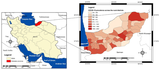
Figure 1.
Location of Golestan province and its 60 rural districts.
2.2. Data Collection and Preparation
The disease data and potentially relevant factors (n = 32) were collected based on previous studies [9,10,11,12]. The prepared dataset includes COVID-19 prevalence per 100,000 population (as the dependent variable) and socio-demographic, environmental, land use, and climatic data as independent variables. Detailed information about the variables is provided in Table 1. ArcGIS 10.2 (ESRI, Redlands, CA, USA) and Microsoft Excel 2016 were used to prepare the dataset at the rural district scale. Continuous raster grids of the climatic data were generated using the inverse distance weighting interpolation method [30]. The zonal statistic function was applied to calculate average values of the digital elevation model (DEM), normalized difference vegetation index (NDVI), and climatic variables at the rural district level. We used the min-max normalization approach [31] for dependent and independent variables to increase the computational performance of models based on Equation (1):
where Xi, Xmin, Xmax, and Xn are the initial, minimum, maximum, and normalized values, respectively.

Table 1.
Summary of the dataset used in this study.
2.3. Statistical Analysis
Initially, the linear regression (LR) method was used to select independent and main variables as inputs for modeling. This method also was used as the baseline to investigate the effects of independent variables on the dependent variable. Tests of tolerance and variance inflation factor (VIF) were applied to examine the multicollinearity of all variables [34]. To conduct the PCA, factor analysis in dimension reduction was employed [35]. In this regard, Kaiser-Meyer-Olkin (KMO) and Bartlett’s tests were used to assess the suitability and adequacy of the data for use in the PCA [15]. All statistical analyses were conducted in the SPSS software version 23.
2.4. ANFIS
The fuzzy theory is an approach to making decisions when dealing with ambiguous and inaccurate data with no explicit criteria and accurate boundaries [36,37]. Although this method is popular among researchers in numerous fields, it does not generate high accuracies in unforeseen circumstances [27]. Due to the learning abilities of the ANN to optimize the fuzzy methods, ANFIS was developed [38]. ANFIS, a combination of the ANN and Takagi-Sugeno fuzzy system, benefits from both the learning ability of ANN and the computational ability of fuzzy methods to solve the optimization issue of nonlinear functions [36]. Neuro-fuzzy models were found beneficial compared to classical models of ANNs in some studies [27,39,40,41]. ANFIS is less dependent on the knowledge of experts, can capture nonlinear structures, is adaptable, and can learn quickly [27].
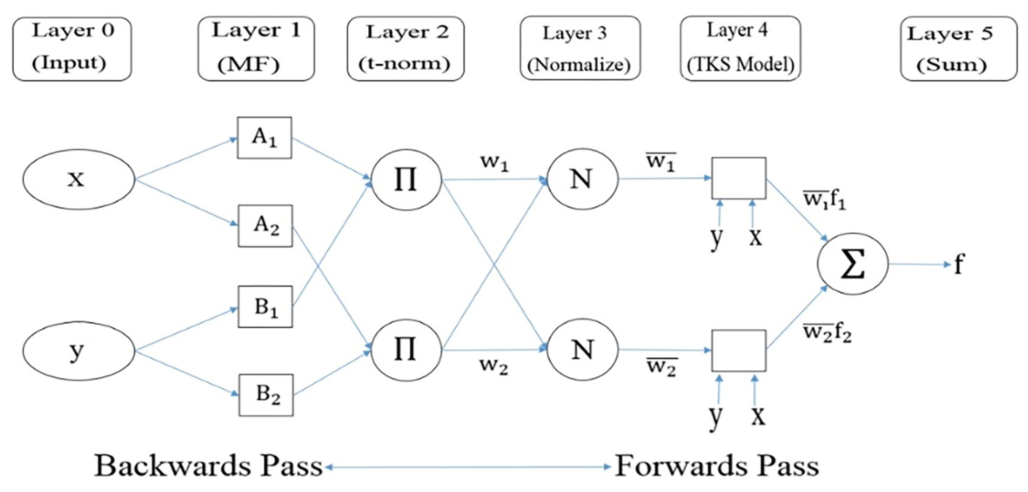
The ANFIS generates a mapping between inputs and outputs by applying fuzzy if-then rules [24]. Figure 2 illustrates the main architecture of the ANFIS with five layers and two inputs x and y (i.e., variables) in the input layer (Layer 0). More information about the structure of ANFIS is presented in [24].
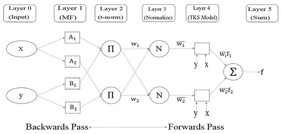
Figure 2.
The primary architecture of the ANFIS [24].
2.5. PCA
It is evident that smaller datasets are easier to visualize and explore; hence, they are faster to be processed. The PCA was first presented by Pearson to reduce the dimensions of a dataset, containing many correlated variables [35,42,43]. Therefore, it preserves the diversity in the dataset to the maximum extent [44] and reduces complexity in the dataset while controlling data loss [26]. In this method, by maximizing the correlation between the variables, the variables are transformed into principal components (PCs). The PCs are the eigenvectors of a covariance matrix and are mutually uncorrelated [35,42]. To apply the PCA-ANFIS model, we decomposed the input variables into PCs and then used them for training the ANFIS model [27]. More information about PCA is presented in [35,42,43].
2.6. Model Development and Evaluation
To implement the ANFIS model, the potentially selected variables (resulted from the LR analysis) and the COVID-19 prevalence were set as independent (inputs) and dependent variables, respectively. The ANFIS model was implemented using the ANFIS toolbox in MATLAB R2015a. In the ANFIS model, three methods of Fuzzy C-means (FCM) clustering, subtractive clustering, and grid partitioning were used to cluster the input data and to facilitate the training phase. However, as FCM clustering usually has shown a better performance than subtractive clustering and grid partitioning [14,45], this method was used in this study. The Gaussian and linear membership functions were employed in the ANFIS model. The parameters of the maximum epoch and error goal were set to thirty and zero, respectively.
We randomly divided the dataset into three categories: training data (52%, thirty-one rural districts), validation data (13%, eight rural districts), and test data (35%, twenty-one rural districts). The training data were considered to calibrate the model, and the validation data were used to avoid overfitting in the training process. The test data were considered to evaluate the ability of the model to predict the target variable. To estimate the model accuracy, four evaluation metrics were used in the model development and evaluation stages: determination coefficient (R2), mean square error (MSE), mean absolute error (MAE), and root mean square error (RMSE) [14,15]. To deal with model uncertainty (i.e., overestimation and underestimation), the training, validation, and test data were set in four different modes. In each mode, we ran the model 5 times. Then, we calculated the average of the results.
In the PCA-ANFIS model, we applied the PCA to extract the PCs. Then, the PCs were considered as inputs for the ANFIS model. To compare the performance of the ANFIS and PCA-ANFIS models, we used the same training, validation, and test data for the above-mentioned models.
Finally, sensitivity analysis was performed to explore the contribution of selected variables in predicting COVID-19 prevalence. In this regard, each factor was removed from the ANFIS model separately for the test data, and the impact of that factor on the model’s accuracy was assessed by the evaluation indicator of R2.
3. Results
Among 32 potential variables, only 17 independent variables were selected as the final input candidates, including average household size, percentage of people over 65 years, migration rate, employment rate, literacy rate, residential apartment units, educational facilities, cultural and sports facilities, religious facilities, municipal services, health facilities, NDVI, maximum wind speed, number of days with rainfall, mean dew point temperature, mean temperature, and mean soil temperature.
3.1. Statistical Analysis
The results of the LR model are presented in Table 2. The linear correlation between the desired and predicted dependent variable was R = 0.697. The R2 = 0.486 shows that 48.6% of total variations in COVID-19 prevalence can be predicted by the selected variables. The value of the Durbin–Watson test was close to two, indicating the independence of the error assumption [14].
Table 2.
The results of the LR model.
Table 3 shows the results of the collinearity of the input factors. The values of tolerance and VIF statistics (tolerance > = 0.1 and 1 < VIF < = 10) imply that multicollinearity is not a major concern. Thus, they can be used in the ANFIS model [15].
Table 3.
Multicollinearity analysis of input variables in the LR model.
The value of the KMO test was 0.719, which indicates the data are sufficient to apply the PCA. In addition, the value of Bartlett’s test (approx. Chi-Square = 709.571) indicates that the data are appropriate for the factor analysis [35].
Among seventeen components, only five components (with eigenvalues > 1) were selected as PCs (Table 4). To optimize the structure of the PCs and equalize their relative importance, we rotated them using the Varma rotation [35,46]. After rotation, the eigenvalues of the PCs were updated and included in the section of rotation sums of the squared loadings. Based on Table 4, the most important PCs in explaining the cumulative variance of the PCs (76.976%) were the PC1 (variance = 29.867%), followed by PC2 (variance = 14.329%), PC3 (variance = 12.341%), PC4 (variance = 11.458%), and PC5 (variance = 8.980%).
Table 4.
Selecting the PCs according to the total variances.
According to Table 5, the varimax rotation with Kaiser Normalization was used to obtain the loading values of each variable for each PC [47], and only the largest absolute value was selected. The variables associated with that value were considered as the candidate variables for the related PCs [35]. The PC1 has a strong positive loading with the percentage of people over 65 years (0.769), residential apartment units (0.739), educational facilities (0.673), cultural and sports facilities (0.813), religious facilities (0.821), health facilities (0.807), NDVI (0.632), and mean dew point temperature (0.580). The PC2 has a negative loading with employment rate (−0.492) and the number of days with rainfall −0.931), while it has a strong positive loading with mean soil temperature (0.910). The PC3 has a strong positive loading with the average household size (0.893) and municipal services (0.676). The PC4 has a strong negative loading with maximum wind speed (−0.839), whereas it has a strong positive loading with the mean temperature (0.835). The PC5 is associated with migration (0.711) and literacy rates (0.799).
Table 5.
The loading of each variable on each PC using the rotated component matrix (rotation converged in 10 iterations). The bold values are associated with the candidate variables for the related PCs.
3.2. Model Evaluation
According to Table 6, the PCA-ANFIS model could explain larger variations in COVID-19 prevalence (mean R2 = 0.615) than the ANFIS model (mean R2 = 0.543) on the test data.
Table 6.
Comparison of predicted COVID-19 prevalence using the ANFIS and PCA-ANFIS models.
3.3. Sensitivity Analysis
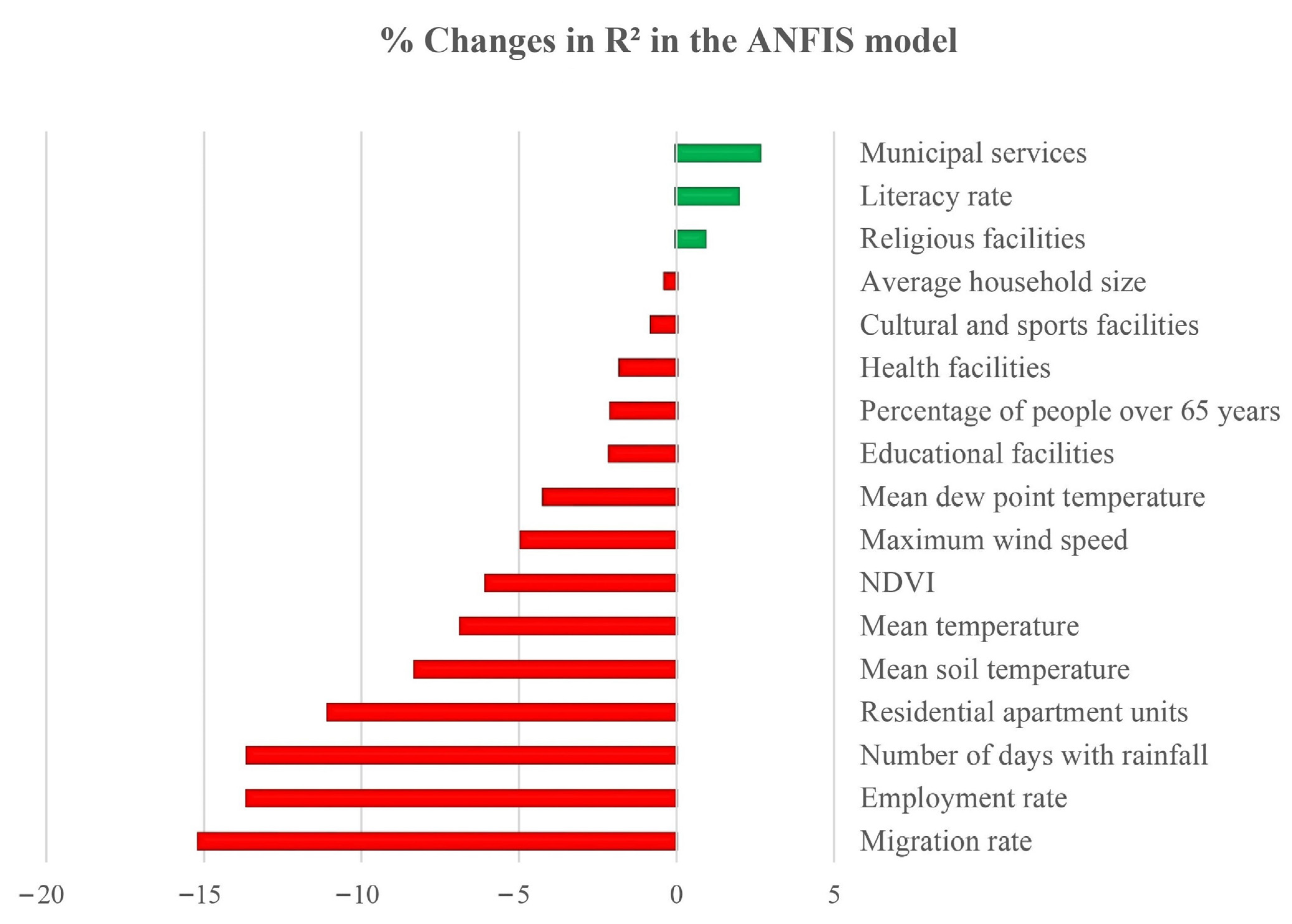
The largest reduction in the R2 occurred when the migration rate (15.16%), the employment rate (13.62%), the number of days with rainfall (13.61%), and residential apartment units (11.05%) were excluded from the ANFIS model. Therefore, these factors are considered the most contributing variables in predicting the geographical distribution of COVID-19 prevalence. Figure 3 depicts the importance of each variable on COVID-19 prevalence.
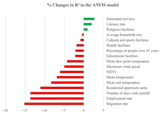
Figure 3.
The contribution of input variables in predicting the spatial distribution of COVID-19 prevalence using the ANFIS model.
4. Discussion
In this study, we assumed that the heterogeneous spatial distribution of COVID-19 prevalence could be explained by socio-demographic, environmental, climatic, and urban land uses factors. We compiled a broad range (n = 32) of these factors to predict COVID-19 prevalence at the rural district level. However, due to the relatively small sample size, traditional modeling techniques could result in overfitting. To address this problem, we used the hybrid neural network and fuzzy logic called ANFIS in a GIS framework. The ANFIS has a robust predictive capability in modeling complex and nonlinear relationships [38]. We further improved the model’s performance [15,27] using PCA. The results of this study will enable policymakers to predict the spatial distribution of COVID-19 and make decisions on designing preventive policies to control future epidemics. In addition, identifying the most contributing factors in COVID-19 prevalence provides valuable insights into the disease transmission, thereby helping more targeted interventions to weaken the spread of the disease.
Among 32 variables, only 17 variables were selected as the inputs for modeling after variable selection. The baseline LR model showed that the selected variables could explain 48.6% of the total variations in COVID-19 prevalence. We improved the performance of the model by at least 13% when using the ANFIS (R2 = 0.543) and PCA-ANFIS (R2 = 0.615) models. This might be due to the ability of ANFIS in capturing nonlinear and linear relationships [14]. The previous literature has implied that nonlinear models had superior performance compared to linear models. For example, [12] indicated that an MLP neural network with one hidden layer (as a nonlinear model) could predict COVID-19 incidence better than an LR model. Reference [11] showed that a combination of the virus optimization algorithm (VOA) with the ANFIS model improves the performance of the ANFIS model in predicting the infection rate of COVID-19. They also indicated that both ANFIS (R2 = 0.691) and ANFIS-VOA models (R2 = 0.834) performed better than LR (R2 = 0.392). Another study stated that RF and ANFIS, as nonlinear models, had higher accuracy in predicting the spatial variation in COVID-19 cases than the logistic regression model (i.e., a generalized linear model) [9]. In line with our results, previous studies also have indicated that the PCA can improve the performance of ML approaches [15,25,26,27,35].
The sensitivity analysis of the ANFIS model showed that four variables of migration rate, employment rate, number of rainfall days, and residential apartment units were among the most contributing factors in predicting COVID-19 prevalence in the Golestan province. The results are consistent with previous studies. For instance, [48,49,50] proposed that the high risk of the spread of COVID-19 was associated with areas with a higher migrant population. Areas with high rates of migrant population can catalyze disease transmission. With the increase in population movements in these areas, the number of people entering and leaving those areas increases. In turn, migrant populations have to travel a greater distance between their residence and workplace, which increases the chance of their contact with other people. It makes the migrant population more likely to contract the virus and causes long-distance transmission of COVID-19. On the other hand, areas with higher populations and higher socio-economic conditions usually attract more migrant people [51]. In this study, according to our census data [29], the rural districts with high migration rates usually had high populations, which can facilitate the COVID-19 transmission in those areas. This suggests the importance of formulating lockdown measures in the early stages of the pandemic to prevent large-scale disease transmission.
Moreover, the previous literature has suggested that a higher employment rate can increase the likelihood of COVID-19 exposure [52,53], particularly when using public transportation to commute to and from the workplace. The proximity of employed people in workplaces, such as offices, can provide a suitable environment for virus transmission. In addition, employed people are usually more exposed to touching infected work surfaces, including keyboards, public toilets, doors, and window handles, as the virus can survive for up to 72 h on high-touch surfaces [54].
Reference [55] assessed the impact of climate factors on COVID-19 transmission. They showed that precipitation, low temperature, dew/frost point, and wind speed escalate the disease incidence. Climate factors, such as low humidity and temperature, may allow the virus to retain its viability longer and subsequently prolong its infectivity [55]. On the other hand, cold and dry weather conditions may also disrupt the human immune response, thereby increasing the risk of disease [55]. In terms of health policy implications, health authorities can adjust their intervention based on different weather conditions. Contrary to the results of this study, some previous research indicated that climatic variables (e.g., temperature and humidity) were not effective in COVID-19 occurrence [10,12,23]. The differences in findings may be attributed to different geographic areas, various methods, and different spatial scales of analysis.
In our study area, the residential apartment units were more concentrated in densely populated urban areas; thus, they were more likely to be exposed to the virus. In agreement with our results, [56] concluded that residential areas are among the most significant urban land uses in the spread of COVID-19. This implies that health authorities should allocate more health resources to the residents of these populated areas to control COVID-19 transmission. To the best of our knowledge, this research is the first attempt to use a comprehensive set of urban land uses for modeling the spatial variations in COVID-19 prevalence, particularly using the ANFIS and PCA-ANFIS. Previous studies have recommended using land use variables in future works [9,11,12].
This study has some limitations that may impede the reliable prediction of the disease distribution. First, although our findings align with some previous studies, interpreting the results at the individual level may not be reliable due to ecological fallacy. Thus, the conclusions can only be drawn at the rural district scale. The lack of some main socio-economic variables (e.g., poverty, race, and insurance status) at the rural district level is another limitation. Moreover, errors and irregularity in the data collection phase can compromise the model’s accuracy. For instance, some cases may be misdiagnosed, or the asymptomatic patients not being reported may lead to unreliable estimations of disease prevalence. Examining data uncertainty should be addressed in future works.
5. Conclusions
Despite the low number of training samples, both the ANFIS and PCA-ANFIS models predicted COVID-19 prevalence in the Golestan province with decent accuracy. Regarding public health implications, the results showed how migration rate, employment rate, and the number of rainfall days could predict COVID-19 prevalence. Moreover, high contributions of residential apartment land use in predicting COVID-19 distribution imply that health authorities should allocate more medical resources to the residents of areas with a higher density of apartment units. To improve the predictability of the ANFIS model, other optimization algorithms, such as equilibrium optimizer algorithm [57], crow search algorithm [58], and Harris Hawks Optimizer [59], can be used in future works. With the increase in the amount of training data, deep learning models can be used, which can lead to higher accuracy of the model. However, the low number of training samples in this study impedes us from using the deeper networks. For future works, by considering a longer time period (if available) or finer spatial scales (which was not possible in this study), we can increase the amount of data and, in turn, adjust the deep learning models [6]. Further studies, such as agent-based models [60,61,62], can be helpful to better understand the complex spatial dynamics of COVID-19 in communities. Nonetheless, this study can be served as a helpful guideline for health policymakers to determine potential risk factors pertaining to COVID-19, particularly for areas with small sample sizes.
Author Contributions
Conceptualization, Mohammad Tabasi, Elnaz Babaie, and Abolfazl Mollalo; methodology, Mohammad Tabasi and Elnaz Babaie; software, Elnaz Babaie; validation, Mohammad Tabasi, Elnaz Babaie, and Abolfazl Mollalo; formal analysis, Mohammad Tabasi and Elnaz Babaie; investigation, Mohammad Tabasi, Elnaz Babaie, and Abolfazl Mollalo; resources, Mohammad Tabasi and Elnaz Babaie; data curation, Mohammad Tabasi; writing—original draft preparation, Mohammad Tabasi; writing—review and editing, all authors; visualization, Mohammad Tabasi and Elnaz Babaie; supervision, Ali Asghar Alesheikh and Mohsen Kalantari; project administration, Ali Asghar Alesheikh. All authors have read and agreed to the published version of the manuscript.
Funding
This research received no external funding.
Institutional Review Board Statement
Not applicable.
Informed Consent Statement
Not applicable.
Data Availability Statement
The data underlying this article will be shared on reasonable request to the corresponding author.
Acknowledgments
The authors gratefully acknowledge the support of the staff of the CDC of the Golestan province for sharing the COVID-19 dataset at the rural district level.
Conflicts of Interest
The authors declare no conflict of interest.
References
- World Health Organization. Novel Coronavirus (2019-nCoV) Situation Reports; World Health Organization: Geneva, Switzerland, 2020. Available online: https://www.who.int/emergencies/diseases/novel-coronavirus-2019/situation-reports (accessed on 4 April 2020).
- World Health Organization. Laboratory Testing Strategy Recommendations for COVID-19. 2020. Available online: https://apps.who.int/iris/bitstream/handle/10665/331509/WHO-COVID-19-lab_testing-2020.1-eng.pdf (accessed on 13 April 2020).
- Ritchie, H.; Mathieu, E.; Rodés-Guirao, L.; Appel, C.; Giattino, C.; Ortiz-Ospina, E.; Hasell, J.; Macdonald, B.; Beltekian, D.; Roser, M. Coronavirus pandemic (COVID-19). Our World Data 2020. Available online: https://ourworldindata.org/coronavirus (accessed on 10 February 2022).
- Abd Elaziz, M.; Dahou, A.; Alsaleh, N.A.; Elsheikh, A.H.; Saba, A.I.; Ahmadein, M. Boosting COVID-19 image classification using MobileNetV3 and aquila optimizer algorithm. Entropy 2021, 23, 1383. [Google Scholar] [CrossRef] [PubMed]
- Issa, M.; Helmi, A.M.; Elsheikh, A.H.; Abd Elaziz, M. A biological sub-sequences detection using integrated BA-PSO based on infection propagation mechanism: Case study COVID-19. Expert Syst. Appl. 2022, 189, 116063. [Google Scholar] [CrossRef]
- Elsheikh, A.H.; Saba, A.I.; Abd Elaziz, M.; Lu, S.; Shanmugan, S.; Muthuramalingam, T.; Kumar, R.; Mosleh, A.O.; Essa, F.A.; Shehabeldeen, T.A. Deep learning-based forecasting model for COVID-19 outbreak in Saudi Arabia. Process Saf. Environ. Prot. 2021, 149, 223–233. [Google Scholar] [CrossRef] [PubMed]
- Saba, A.I.; Elsheikh, A.H. Forecasting the prevalence of COVID-19 outbreak in Egypt using nonlinear autoregressive artificial neural networks. Process Saf. Environ. Prot. 2020, 141, 1–8. [Google Scholar] [CrossRef]
- Al-Qaness, M.A.; Saba, A.I.; Elsheikh, A.H.; Abd Elaziz, M.; Ibrahim, R.A.; Lu, S.; Hemedan, A.A.; Shanmugan, S.; Ewees, A.A. Efficient artificial intelligence forecasting models for COVID-19 outbreak in Russia and Brazil. Process Saf. Environ. Prot. 2021, 149, 399–409. [Google Scholar] [CrossRef] [PubMed]
- Razavi-Termeh, S.V.; Sadeghi-Niaraki, A.; Farhangi, F.; Choi, S.M. COVID-19 Risk Mapping with Considering Socio-Economic Criteria Using Machine Learning Algorithms. Int. J. Environ. Res. Public Health 2021, 18, 9657. [Google Scholar] [CrossRef] [PubMed]
- Mollalo, A.; Vahedi, B.; Rivera, K.M. GIS-based spatial modeling of COVID-19 incidence rate in the continental United States. Sci. Total Environ. 2020, 728, 138884. [Google Scholar] [CrossRef]
- Behnood, A.; Golafshani, E.M.; Hosseini, S.M. Determinants of the infection rate of the COVID-19 in the US using ANFIS and virus optimization algorithm (VOA). Chaos Solitons Fractals 2020, 139, 110051. [Google Scholar] [CrossRef]
- Mollalo, A.; Rivera, K.M.; Vahedi, B. Artificial neural network modeling of novel coronavirus (COVID-19) incidence rates across the continental United States. Int. J. Environ. Res. Public Health 2020, 17, 4204. [Google Scholar] [CrossRef]
- Tabasi, M.; Alesheikh, A.A. Spatiotemporal variability of Zoonotic Cutaneous Leishmaniasis based on sociodemographic heterogeneity. The case of Northeastern Iran, 2020, 2011–2016. Jpn. J. Infect. Dis. 2021, 74, 7–16. [Google Scholar] [CrossRef]
- Babaie, E.; Alesheikh, A.A.; Tabasi, M. Spatial prediction of human brucellosis (HB) using a GIS-based adaptive neuro-fuzzy inference system (ANFIS). Acta Trop. 2021, 220, 105951. [Google Scholar] [CrossRef]
- Babaie, E.; Alesheikh, A.A.; Tabasi, M. Spatial modeling of zoonotic cutaneous leishmaniasis with regard to potential environmental factors using ANFIS and PCA-ANFIS methods. Acta Trop. 2022, 228, 106296. [Google Scholar] [CrossRef]
- Jin, B.; Ji, J.; Yang, W.; Yao, Z.; Huang, D.; Xu, C. Analysis on the spatio-temporal characteristics of COVID-19 in mainland China. Process Saf. Environ. Prot. 2021, 152, 291–303. [Google Scholar] [CrossRef] [PubMed]
- Snyder, B.F.; Parks, V. Spatial variation in socio-ecological vulnerability to Covid-19 in the contiguous United States. Health Place 2020, 66, 102471. [Google Scholar] [CrossRef]
- Li, D.; Chaudhary, H.; Zhang, Z. Modeling spatiotemporal pattern of depressive symptoms caused by COVID-19 using social media data mining. Int. J. Environ. Res. Public Health 2020, 17, 4988. [Google Scholar] [CrossRef] [PubMed]
- Hossam, A.; Magdy, A.; Fawzy, A.; El-Kader, A.; Shriene, M. An integrated IoT system to control the spread of COVID-19 in Egypt. In Proceedings of the International Conference on Advanced Intelligent Systems and Informatics, Cairo, Egypt, 19–21 October 2020; Springer: Cham, Switzerland, 2020; pp. 336–346. [Google Scholar]
- Martellucci, C.A.; Sah, R.; Rabaan, A.A.; Dhama, K.; Casalone, C.; Arteaga-Livias, K.; Sawano, T.; Ozaki, A.; Bhandari, D.; Higuchi, A.; et al. Changes in the spatial distribution of COVID-19 incidence in Italy using GIS-based maps. Ann. Clin. Microbiol. Antimicrob. 2020, 19, 30. [Google Scholar] [CrossRef]
- Urban, R.C.; Nakada, L.Y.K. GIS-based spatial modelling of COVID-19 death incidence in São Paulo, Brazil. Environ. Urban. 2021, 33, 229–238. [Google Scholar] [CrossRef]
- Murugesan, B.; Karuppannan, S.; Mengistie, A.T.; Ranganathan, M.; Gopalakrishnan, G. Distribution and trend analysis of COVID-19 in India: Geospatial approach. J. Geogr. Stud. 2020, 4, 1–9. [Google Scholar] [CrossRef]
- Razavi-Termeh, S.V.; Sadeghi-Niaraki, A.; Choi, S.M. Coronavirus disease vulnerability map using a geographic information system (gis) from 16 april to 16 may 2020. Phys. Chem. Earth Parts A/B/C 2021, 126, 103043. [Google Scholar] [CrossRef]
- Jang, J.-S.; Sun, C.-T. Neuro-fuzzy modeling and control. Proc. IEEE 1995, 83, 378–406. [Google Scholar] [CrossRef]
- Çaydaş, U.; Hasçalık, A.; Ekici, S. An adaptive neuro-fuzzy inference system (ANFIS) model for wire-EDM. Expert Syst. Appl. 2009, 36, 6135–6139. [Google Scholar] [CrossRef]
- Bartoletti, N.; Casagli, F.; Marsili-Libelli, S.; Nardi, A.; Palandri, L. Data-driven rainfall/runoff modelling based on a neuro-fuzzy inference system. Environ. Model. Softw. 2018, 106, 35–47. [Google Scholar] [CrossRef]
- Razin, M.R.G.; Voosoghi, B. Ionosphere time series modeling using adaptive neuro-fuzzy inference system and principal component analysis. GPS Solut. 2020, 24, 51. [Google Scholar] [CrossRef]
- COVID-19 Cases Data in Golestan Province. 2020–2021. In Iranian Ministry of Health, Center for Disease Control and Prevention (CDC) of Golestan Province; Unpublished data; 2021; Available online: https://goums.ac.ir/index.php?slc_lang=en&sid=200 (accessed on 28 February 2021).
- Census Data and Land Use data in Golestan Province. 2020–2021. In Statistical Center of Iran, Deputy of Statistics and Information of Golestan Province; 2021; Available online: https://amar.golestanmporg.ir/ (accessed on 10 February 2022).
- Watson, D.F.; Philip, G.M. A refinement of inverse distance weighted interpolation. Geo-Processing 1985, 2, 315–327. [Google Scholar]
- Nor, N.M.; Hussain, M.A.; Hassan, C.R.C. Multi-scale kernel Fisher discriminant analysis with adaptive neuro-fuzzy inference system (ANFIS) in fault detection and diagnosis framework for chemical process systems. Neural Comput. Appl. 2019, 32, 9283–9297. [Google Scholar] [CrossRef]
- United States Geological Survey (USGS). 2020–2021. Available online: https://earthexplorer.usgs.gov/ (accessed on 10 February 2022).
- Meteorological data in Golestan Province. 2020–2021. In Meteorological Organization of Iran; 2021; Available online: https://data.irimo.ir/ (accessed on 10 February 2022).
- Mihanovic, D.; Hunjet, A.; Primorac, Z. Economic and Social Development (Book of Proceedings). In Proceedings of the 18th International Scientific Conference on Economic and Social, Bangkok, Thailand, 18–20 February 2016. [Google Scholar]
- Ul-Saufie, A.Z.; Yahaya, A.S.; Ramli, N.A.; Rosaida, N.; Hamid, H.A. Future daily PM10 concentrations prediction by combining regression models and feedforward backpropagation models with principle component analysis (PCA). Atmos. Environ. 2013, 77, 621–630. [Google Scholar] [CrossRef]
- Uğuz, H. Adaptive neuro-fuzzy inference system for diagnosis of the heart valve diseases using wavelet transform with entropy. Neural Comput. Appl. 2012, 21, 1617–1628. [Google Scholar] [CrossRef]
- Dehnavi, A.; Aghdam, I.N.; Pradhan, B.; Varzandeh, M.H.M. A new hybrid model using step-wise weight assessment ratio analysis (SWARA) technique and adaptive neuro-fuzzy inference system (ANFIS) for regional landslide hazard assessment in Iran. Catena 2015, 135, 122–148. [Google Scholar] [CrossRef]
- Chen, W.; Panahi, M.; Pourghasemi, H.R. Performance evaluation of GIS-based new ensemble data mining techniques of adaptive neuro-fuzzy inference system (ANFIS) with genetic algorithm (GA), differential evolution (DE), and particle swarm optimization (PSO) for landslide spatial modelling. Catena 2017, 157, 310–324. [Google Scholar] [CrossRef]
- Polykretis, C.; Chalkias, C.; Ferentinou, M. Adaptive neuro-fuzzy inference system (ANFIS) modeling for landslide susceptibility assessment in a Mediterranean hilly area. Bull. Eng. Geol. Environ. 2019, 78, 1173–1187. [Google Scholar] [CrossRef]
- Rezaeianzadeh, M.; Tabari, H.; Arabi Yazdi, A.; Isik, S.; Kalin, L. Flood flow forecasting using ANN, ANFIS and regression models. Neural Comput. Appl. 2014, 25, 25–37. [Google Scholar] [CrossRef]
- Moghaddamnia, A.; Gousheh, M.G.; Piri, J.; Amin, S.; Han, D. Evaporation estimation using artificial neural networks and adaptive neuro-fuzzy inference system techniques. Adv. Water Resour. 2009, 32, 88–97. [Google Scholar] [CrossRef]
- Fung, C.-P.; Kang, P.-C. Multi-response optimization in friction properties of PBT composites using Taguchi method and principle component analysis. J. Mater. Processing Technol. 2005, 170, 602–610. [Google Scholar] [CrossRef]
- Warne, K.; Prasad, G.; Siddique, N.H.; Maguire, L.P. Development of a hybrid PCA-ANFIS measurement system for monitoring product quality in the coating industry. In Proceedings of the 2004 IEEE International Conference on Systems, Man and Cybernetics, The Hague, The Netherlands, 10–13 October 2004; (IEEE Cat. No. 04CH37583). Volume 4, pp. 3519–3524. [Google Scholar]
- Jolliffe, I.T. Principal Component Analysis; Springer: New York, NY, USA, 2002. [Google Scholar]
- Benmouiza, K.; Cheknane, A. Clustered ANFIS network using fuzzy c-means, subtractive clustering, and grid partitioning for hourly solar radiation forecasting. Theor. Appl. Climatol. 2018, 137, 31–43. [Google Scholar] [CrossRef]
- Kaiser, H.F. The varimax criterion for analytic rotation in factor analysis. Psychometrika 1958, 23, 187–200. [Google Scholar] [CrossRef]
- Liu, C.-W.; Lin, K.-H.; Kuo, Y.-M. Application of factor analysis in the assessment of groundwater quality in a blackfoot disease area in Taiwan. Sci. Total Environ. 2003, 313, 77–89. [Google Scholar] [CrossRef]
- Liang, Z.; Wang, Y.; Sun, F.; Liang, C.; Li, S. Geographical pattern of COVID-19 incidence of China’s cities: Role of migration and socioeconomic status. Res. Environ. Sci. 2020, 33, 1571–1578. [Google Scholar]
- Fan, C.; Cai, T.; Gai, Z.; Wu, Y. The relationship between the migrant population’s migration network and the risk of COVID-19 transmission in China—Empirical analysis and prediction in prefecture-level cities. Int. J. Environ. Res. Public Health 2020, 17, 2630. [Google Scholar] [CrossRef]
- Xing, G.R.; Li, M.T.; Li, L.; Sun, G.Q. The impact of population migration on the spread of COVID-19: A case study of Guangdong province and Hunan province in China. Front. Phys. 2020, 8, 488. [Google Scholar] [CrossRef]
- Yaojun, Z.; Qiao, C. Spatial patterns of population mobility and determinants of inter-provincial migration in China. Popul. Res. 2014, 38, 54. [Google Scholar]
- Castex, G.; Dechter, E.; Lorca, M. COVID-19: The impact of social distancing policies, cross-country analysis. Econ. Disasters Clim. Chang. 2021, 5, 135–159. [Google Scholar] [CrossRef] [PubMed]
- Millett, G.A.; Jones, A.T.; Benkeser, D.; Baral, S.; Mercer, L.; Beyrer, C.; Honermann, B.; Lankiewicz, E.; Mena, L.; Crowley, J.S.; et al. Assessing differential impacts of COVID-19 on black communities. Ann. Epidemiol. 2020, 47, 37–44. [Google Scholar] [CrossRef]
- Lee, N.R. Reducing the spread of COVID-19: A social marketing perspective. Soc. Mark. Q. 2020, 26, 259–265. [Google Scholar] [CrossRef]
- Sarkodie, S.A.; Owusu, P.A. Impact of meteorological factors on COVID-19 pandemic: Evidence from top 20 countries with confirmed cases. Environ. Res. 2020, 191, 110101. [Google Scholar] [CrossRef]
- Xu, J.; Deng, Y.; Yang, J.; Huang, W.; Yan, Y.; Xie, Y.; Li, Y.; Jing, W. Effect of Population Migration and Socioeconomic Factors on the COVID-19 Epidemic at County Level in Guangdong, China. Front. Environ. Sci. 2022, 10, 27. [Google Scholar] [CrossRef]
- Zayed, M.E.; Zhao, J.; Li, W.; Elsheikh, A.H.; Abd Elaziz, M. A hybrid adaptive neuro-fuzzy inference system integrated with equilibrium optimizer algorithm for predicting the energetic performance of solar dish collector. Energy 2021, 235, 121289. [Google Scholar] [CrossRef]
- Abd Elaziz, M.; Elsheikh, A.H.; Sharshir, S.W. Improved prediction of oscillatory heat transfer coefficient for a thermoacoustic heat exchanger using modified adaptive neuro-fuzzy inference system. Int. J. Refrig. 2019, 102, 47–54. [Google Scholar] [CrossRef]
- Shehabeldeen, T.A.; Abd Elaziz, M.; Elsheikh, A.H.; Zhou, J. Modeling of friction stir welding process using adaptive neuro-fuzzy inference system integrated with harris hawks optimizer. J. Mater. Res. Technol. 2019, 8, 5882–5892. [Google Scholar] [CrossRef]
- Tabasi, M.; Alesheikh, A.A. Development of an agent-based model for simulation of the spatiotemporal spread of Leishmaniasis in GIS (case study: Maraveh Tappeh). J. Geomat. Sci. Technol. 2019, 8, 113–131. [Google Scholar]
- Tabasi, M.; Alesheikh, A.A. Modeling Spatial Spread of Epidemic Diseases using Agent-based Simulation (Case Study: Seasonal Influenza). J. Geomat. Sci. Technol. 2017, 6, 75–86. [Google Scholar]
- Tabasi, M.; Alesheikh, A.A.; Sofizadeh, A.; Saeidian, B.; Pradhan, B.; AlAmri, A. A spatio-temporal agent-based approach for modeling the spread of zoonotic cutaneous leishmaniasis in northeast Iran. Parasites Vectors 2020, 13, 1–17. [Google Scholar] [CrossRef] [PubMed]

Publisher’s Note: MDPI stays neutral with regard to jurisdictional claims in published maps and institutional affiliations. |
© 2022 by the authors. Licensee MDPI, Basel, Switzerland. This article is an open access article distributed under the terms and conditions of the Creative Commons Attribution (CC BY) license (https://creativecommons.org/licenses/by/4.0/).