Abstract
The ability to quickly calculate or query the shortest path distance between nodes on a road network is essential for many real-world applications. However, the traditional graph traversal shortest path algorithm methods, such as Dijkstra and Floyd–Warshall, cannot be extended to large-scale road networks, or the traversal speed on large-scale networks is very slow, which is computational and memory intensive. Therefore, researchers have developed many approximate methods, such as the landmark method and the embedding method, to speed up the processing time of graphs and the shortest path query. This study proposes a new method based on landmarks and embedding technology, and it proposes a multilayer neural network model to solve this problem. On the one hand, we generate distance-preserving embedding for each node, and on the other hand, we predict the shortest path distance between two nodes of a given embedment. Our approach significantly reduces training time costs and is able to approximate the real distance with a relatively low Mean Absolute Error (MAE). The experimental results on a real road network confirm these advantages.
1. Introduction
In the context of a large-scale road network [,] with a large number of users sending out remote distance queries at the same time, determining how to provide a timely response to such a large number of queries is a very important research question for many navigation applications. The aforementioned problem of efficiently and accurately predicting the shortest path distance between nodes in a road network [,] has attracted researchers’ attention, and a number of exact methods [,,,,] capable of performing error-free distance prediction have been proposed, as well as approximate methods [,,,,] that sacrifice some prediction accuracy to reduce computation and memory costs.
The traditional Dijkstra algorithm [] has a time complexity of and a space complexity of , using big O notation [], where and are the number of edges and the number of nodes in the graph, respectively. Moreover, the Floyd–Warshall [] algorithm has a time complexity of and a space complexity of . Such a time complexity is acceptable for small graphs, but for large million-node graphs, the calculation of a single node distance requires massive computational resources and time []. In order to speed up the query times compared with traditional methods, a number of labeling methods have been proposed [,,], all of which use distance labels. The basic idea is to calculate the distance from each node to other nodes (in extreme cases, this may be all the remaining nodes) in advance in the data preprocessing stage in order to form a tuple as the distance label of the node. Then, by checking the distance label, the distance between any two nodes can be calculated in time. However, the difficulty of these labeling methods is to find the minimum node set that needs to calculate and store the distance so as to accurately calculate all the shortest paths. Finding the optimal node set of a graph has been proved to be an NP-hard problem. At the same time, the memory cost consumed by these methods is still [].
In order to reduce the memory cost, researchers proposed approximate shortest path distance methods [,], which further reduce the memory and computation costs by sacrificing some prediction accuracy. The sacrifice is worthwhile, because in many practical applications, or some special graphs (large road network graphs), if the exact distance is not necessary, it is enough to find the approximate distance between nodes. A typical representative of the approximate shortest path distance method is the landmark-based method [,,,]. This method usually selects nodes as landmarks, and then, similar to the marking method, assigns a distance label to each node, which contains the distance from the node to these landmark nodes. When querying the distance between any two nodes, the approximation is the sum of the minimum distances between these two nodes and the same landmark node. Although the landmark-based methods can reduce the memory cost to , these methods cannot guarantee the approximation quality in theory [], and the accuracy of the prediction distance largely depends on the selection of landmarks. Therefore, landmark selection is critical to improve the landmark-based method, but it is also NP-hard [] to select the best landmarks.
The embedding method [,,,] is another representative approximate shortest path distance method. In the data preprocessing stage, this method learns the vector embedding of each node through embedding technology [,,,] to maintain the shortest path distance; that is, each node is embedded into the -dimensional mapping space, such as Euclidean space [] and hyperbolic space [], to calculate the shortest path distance between nodes. Therefore, each node has a corresponding -dimensional embedding vector. When querying the distance, the embedding method uses a more effective distance approximation function, such as directly calculating the -norm between the embedding vectors or training the neural network to predict the distance according to the embedding vectors and the pre-calculated real shortest path distance. It is precisely because of this that the embedding method can make the query speed faster than other approximation methods. In addition, different embedding technologies, embedding dimensions and embedding spaces have a great impact on the accuracy of prediction distance. Therefore, it is also a challenging problem to select the appropriate embedding technology, dimension and space for different graph data.
Inspired by the above approximate shortest path distance methods, such as the landmark-based method and the embedding method, we proposed a new approximate shortest path distance model based on neural networks. The model integrates the landmark-based method, the embedding method and a neural network model, which greatly reduces the time cost by training.
The remainder of the paper is structured as follows: The preliminary knowledge and related work are reviewed in Section 2. Section 3 introduces our model ndist2vec in detail. We arrange the experiment in Section 4, and we describe the experimental dataset, evaluation index, experimental parameters and experimental results. Finally, conclusions are drawn in Section 5.
2. Preliminary Knowledge and Related Work
2.1. Preliminary Knowledge
Let be an undirected road network graph with nodes and edges. For each node (road intersection), has a pair of geocoordinates, and the edge (roads) connects nodes and , indicating that they are adjacent and have the weight , which represents the distance across the edge, i.e., the distance between the two road intersections. Figure 1 shows an example, which contains nodes and edges; and are two nodes of the graph, and the presence of edge shows that they are adjacent and have the weight , indicating that the distance between them is .

Figure 1.
An example of undirected road network graph.
Given node and node , there exists at least one path ; this is connected by a series of adjacent nodes, which can make reach . The path length is the sum of the weights between these series of nodes. For example, there are three paths from node to node , which are , and , and the corresponding path lengths are , and , respectively. We specify that the shortest path between node and node is and that denotes the real shortest path length, so for node and node , the shortest path length is .
2.2. Related Work
Researchers at the University of Passau proposed a new method [] for approximating the shortest path distance between two nodes in a social graph based on a landmark approach, and they used simple neural networks with node2vec [] or Poincare [] embeddings and obtained better results than Orion and Rigel on a social graph dataset. For convenience, we name this method node2vec-Sg. In detail, in the first step, they utilized node embedding technology to learn the vector embedding of each node in the graph. In the second step, they extracted training sample pairs in the entire graph . They randomly selected ) nodes from as landmarks, and they applied the breadth-first search (BFS) algorithm to calculate the true distance from each landmark node to the remaining nodes so as to obtain sample pairs similar to . In order to approximately calculate the distance between two nodes, and , they combined their embeddings, and , through some binary operation (the operations included subtraction, averaging, multiplication or concatenating between vectors) so as to form a training sample pair, such as . Finally, the feedforward neural network composed of a single hidden layer was trained through these training samples, and the neural network output the actual value prediction of the shortest path distance . The specific process is shown in Figure 2.
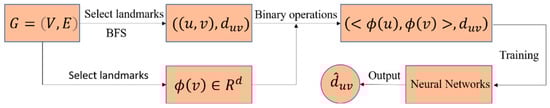
Figure 2.
Base architecture of node2vec-Sg.
In addition, since the neural network performs a regression task, the Mean Square Error (MSE) is used as the loss function, and the Stochastic Gradient Descent (SGD) [] is used as the optimizer. In all their experiments, they confirmed that the node2vec embedding gives better results than the Poincare embedding, adding that the node2vec embedding is not able to learn the structural features of distant nodes, so it is not suitable for graphical structures with many distant nodes, such as road networks.
Researchers have proposed a learning-based model called vdist2vec []. The model can effectively and accurately predict the shortest path distance between two nodes in a road network, and the distance prediction time and the storage space of the model are and , respectively, in which is the dimension of node embedding. As shown in Figure 3, in the -dimensional one-hot layer, vdist2vec takes the -dimensional one-hot vectors and of nodes and as inputs, and the next layer is an embedding layer composed of nodes. In this layer, the embedding of each node is learned to generate the weight matrix . Through the formula , the embedding of each node can be obtained; in this case, and are obtained, and then . and are connected as input to train a multilayer perceptron (MLP) in order to predict the shortest path distance for a given embedding of two nodes. Moreover, researchers have proposed improved models vdist2vec-L and vdist2vec-S of the base model vdist2vec, where vdist2vec-L uses Huber loss as the loss function and is able to reduce more errors than the base model vdist2vec, which uses the Mean Square Error (MSE). The model vdist2vec-S is driven by ensemble learning. Four independent MLPs are replaced with the last hidden layer of vdist2vec to focus on the distances in different ranges, and their outputs are added to obtain the final distance prediction.
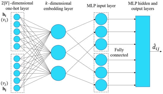
Figure 3.
Base architecture of vdist2vec.
The above models achieve fast distance prediction without increasing the spatial cost. The advantages of the three models have been confirmed in experiments on several different real road networks, and vdist2vec-S is the best one of the three models. However, in order to better learn the node embeddings and to obtain a higher prediction accuracy, the models use all node pairs as training samples to train the neural network, thus significantly increasing the training time. Inspired by the above-mentioned use of embedding methods and landmark-based methods in the approximate shortest path distance problem, we propose a new approximate shortest path distance prediction model, ndist2vec. The goal is to maintain a relatively high prediction accuracy and fast query time while greatly reducing the training time. In the next section, we elaborate on the details of ndist2vec.
3. Ndist2vec
In this section, we proposed the ndist2vec model. As shown in Figure 4, we used the method of randomly selecting landmarks to divide the set of nodes into a set of landmark nodes and a set of remaining nodes . Then, our ndist2vec model selects two nodes, and , and obtains their corresponding embedding vectors, and , respectively, by using the vector embedding matrix (each node has a corresponding embedding vector), and it finally connects the vectors and as input to train a multilayer neural network to output the distance between the two given nodes, and .
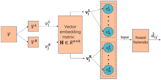
Figure 4.
Base architecture of ndist2vec.
Specifically, our goal was to extract training pairs from the entire graph to train a multilayer neural network and then to predict the shortest path distance between any two nodes and in a graph . In the first stage, we selected (where ) nodes in the node set as landmarks and generated the set of landmark nodes , and the remaining nodes in generated the set of remaining nodes ; i.e., the set is divided into sets and (where and ). In the second stage, we randomly initialized a vector embedding matrix so that we could obtain an embedding vector for each node . Since our embeddings can be guided directly by distance prediction, we can update based on the back propagation of the training predictions for each epoch, which also means updating each embedding vector . In the third stage, using the vector embedding matrix , we could obtain the embedding vector corresponding to node of the landmark node set and the embedding vector corresponding to node of the remaining node set , and we connected them together as training samples while calculating the actual shortest path distance of these two nodes as the supervision information (label) of this sample. Then, we utilized the above method to traverse each landmark node and the remaining nodes to obtain training samples, along with their corresponding supervision information. Finally, the training samples were used as input to a multilayer neural network. The neural network maps the input training samples to real-valued distances.
As shown in Figure 5, we designed a four-layer neural network consisting of an input layer, two hidden layers and an output layer. The size of the input layer depends on the dimension of the vector embedding, and since two vectors are connected in series, neurons are required. Since the ReLU [] function is effective in training neural networks, we set the activation function for the first three layers to the ReLU function. In the output layer, we learned the distances in different ranges in the form of ensemble learning, and we added their outputs to obtain the final distance prediction.
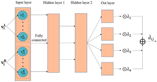
Figure 5.
Base architecture of neural networks.
We used the Mean Square Error (MSE) to measure the quality of the predictor because the network performs a regression task, so the Mean Square Error of the actual node distance and the predicted distance was taken as our training loss function :
Finally, we used adaptive moment estimation (ADAM) [] as an optimizer, which controls the learning rate after bias correction with a defined range of learning rates per iteration. We made the parameters relatively smooth, and their effectiveness has been verified in a large number of deep neural network experiments. During training, all parameters of the neural network are randomly initialized. The training samples are fed into the network in batches for training. The training loss is passed back to optimize all parameters in the network.
4. Experiment
In this section, we tested our proposed ndist2vec on four road network datasets and compared it with node2vec-sg and vdis2vec. All these methods were implemented by Python 3.7 on a PC with an Intel Core Duo Processor (double 4.2 GHz) with 16 GB RAM. Next, we first described the datasets, some parameter settings and evaluation metrics; then, we described the experiments that we conducted and presented the results; and, finally, we presented the conclusions drawn from the experimental results and the reasons why they turned out the way they did. The source code of the program and the experimental data were archived on figshare [].
4.1. Datasets and Hyperparameters
We used four different road network graphs [] for the experiments. We extracted the maximum connected component from these road graphs, renamed the node name and specified the coordinates. Therefore, all datasets contain weighted edges and unique map coordinates for each node. In addition, they are all undirected, and the number of nodes , number of edges , the maximum distance , the minimum distance and the average distance between the nodes are summarized in Table 1, and Figure 6 shows the original road network.

Table 1.
Statistics of road network datasets.
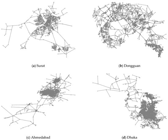
Figure 6.
Road networks.
For all comparison methods, we used their recommended hyperparameter settings. In our ndist2vec model, the neural network consists of four layers: an input layer containing neurons; an output layer containing neuron; and two hidden layers containing and neurons, respectively, where is the embedding dimension, and we set . The four parameters of ensemble learning, were randomly initialized and updated with each epoch of training. The model was trained for a total of epochs. All sample pairs were trained in the first epoch, and in the remaining epochs, landmarks were randomly re-generated for each epoch; i.e., sample pairs were trained for each epoch, and all epochs were trained at a learning rate of .
We used two types of metrics to measure the accuracy and speed of our method. Firstly, we utilized the Mean Absolute Error (MAE) and the Mean Relative Error (MRE) to measure the difference between our predicted value and the real value . Their definitions are
and
respectively, and the smaller the value, the higher the accuracy. Secondly, we used the training time (PT) and the average distance prediction time (AT) to measure the speed of the model. In our experiment, our prediction set consists of pairs of all nodes.
4.2. Overall Results
Table 2 shows the experimental results of the prediction error and time cost of ndist2vec, vdist2vec-S and node2vec-Sg on the four road network datasets. In terms of the prediction error, it can be seen that vdist2vec-S has the smallest MAE and MRE for each dataset because it learns all node pair information and retains the distance information of the node pairs through node embedding (Bolded numbers indicate best performance). Our method ndist2vec has a larger MAE and MRE than those of vdist2vec-S, but the size is limited. We used the landmark-based method for learning, and we did not learn all the node pair information but retained the node embedding information in the vector embedding matrix. Node2vec-Sg is an approximate method for predicting the shortest path distance of social networks. We changed its weight to the real distance and carried out experiments on road networks, but we did not obtain good results. The reason is that node2vec-Sg sometimes oversamples and undersamples in the process of generating training samples; that is, the samples are not evenly divided, and not all node pair information is learned. At the same time, the embedding technology node2vec is not suitable for road network nodes; this is explained in our subsequent experiments.
Table 2.
Experimental results of three models.
In terms of the training time cost PT, our method ndist2vec has the best performance. The advantage of our model is that it sacrifices some accuracy to greatly reduce the training time, and this accuracy sacrifice is worthwhile. Specifically, for the datasets SU, AH and DH, the MAEs of ndist2vec are , and times those of vdist2vec-s, respectively, but the training time PT is at least one-quarter of that of vdis2vec-S. Moreover, with an increase in the number of nodes (, the time gap will become increasingly larger. Although node2vec-Sg is also a landmark-based method, it is very time consuming because of the different ways of selecting training samples.
The average prediction time AT is calculated by dividing the total prediction time of all node pairs of samples by the number of sample pairs ) of all the nodes, and the unit is microseconds (μs). The three models need to link the embedded vectors of two nodes in the prediction distance and input them into the corresponding neural network (the neural network structure of the three methods is similar) for forward propagation to obtain the prediction results. It can be seen that the AT of ndist2vec for the four datasets is the smallest. This is because the vector embedding dimension of ndist2vec is always , while the embedding dimension of vdist2vec-S is , and the dimension of node2vec is ; more dimensions will increase the training time PT and the average prediction time AT.
Ndist2vec performs the worst in terms of prediction error in the Dongguan dataset. This is because although the Dongguan dataset only has nodes, a total of about million sample pairs, its average distance between nodes is the highest, m. It is conceivable that the node distribution in the Dongguan dataset is dominated by a large distance. In addition, our method is based on landmarks. We did not learn all the sample pairs during training, so we lack the learning of large-distance sample pairs. Therefore, our method may not be suitable for datasets with large distances between nodes, and this will be our next breakthrough direction.
Our training strategy is to train epochs. The first epoch trains all sample pairs, the remaining epochs train landmark sample pairs, and landmarks are randomly selected again in each epoch. In addition, our vector embedding matrix is updated according to the prediction results. Using the control variable method, we summarized the four models in Table 3 and compared them in Table 4 to verify the effectiveness of our model training strategy.
Table 3.
Model settings.
Table 4.
Comparison results of ndist2vec and three variant models.
Table 3 shows the training settings of the different models. Embedding represents the form of the vector embedding matrix, L indicates that the vector embedding matrix can be updated through the prediction results (that is, our method), and N indicates that the vector embedding matrix is learned in advance according to node2vec embedding technology and will not change with the prediction results. Epoch has two choices. Epoch1 indicates that the first epoch trains all sample pairs, and the remaining 29 epochs train landmark sample pairs; Epoch2 indicates that 30 epochs train landmark sample pairs. The S in Landmark indicates that each epoch generates new landmark sample pairs to participate in training, and F indicates that the landmark is generated once and fixed to participate in all epochs training; that is, each epoch is trained with fixed landmark sample pairs.
Table 4 shows the experimental results of ndist2vec and the other variant models. Specifically, by comparing ndist2vec and ndist2vec-1, we can see that for the four datasets, the result of ndist2vec is better than that of ndist2vec-1, which shows that the method of updating the vector embedding matrix according to the prediction results is more suitable for the prediction of the shortest path distance of a road rather than directly using node2vec embedding technology. Node2vec embedding technology pays more attention to capturing the similarity between nodes, but the shortest path prediction of the road network pays more attention to the distance relationship between nodes. Therefore, the method of updating the vector embedding matrix according to the prediction results is more appropriate to capture the characteristics of the road network. It measures the distance between the nodes rather than the similarity.
Ndist2vec trained all sample pairs in the first epoch, while ndist2vec-2 used the landmark-based method in the first epoch and only trained sample pairs. As a result, the training time PT of ndist2vec was higher than that of ndist2vec-2 (only higher in the first epoch time of training), but the MAE and MRE were reduced. The reason for this is that, although the landmark-based method can reduce the training time, we used the random landmark selection method, which may not generate better sample pairs for training in the first epoch, and then we updated the vector embedding matrix . However, training all sample pairs in the first epoch can better teach and update the vector embedding matrix and provide a good foundation for the next epochs of training.
Comparing the ndist2vec model and the ndist2vec-3 model, in the landmark-based training epoch (the remaining 29 epochs), BB repeats learning 29 times for sample pairs, so it can only learn the information of sample pairs. When the random landmark selection is not good, the performance of ndis2vec-3 deteriorates. However, in the epoch landmark-based training of the ndist2vec model, each epoch randomly selects new landmarks and generates new sample pairs for training; that is, the ndist2vec model can learn more information of sample pairs (where is the set of sample pairs generated by the combination of and ). For regression tasks, the more information used for learning means better fitting. Therefore, it can be seen in Table 4 that ndist2vec performs better than ndis2vec-3.
4.3. Discussion
In this paper, we studied undirected road networks. In fact, in a directed road network, whether all nodes are bidirectionally connected determines whether our model is feasible. When all nodes are bidirectionally connected, a feasible solution for our model in directed road networks is to change the connection order of the node embedding vectors and to train two prediction models in order to predict the bidirectional node distances separately. Currently, we cannot come up with a solution to apply this model to a case where only some nodes are bidirectionally connected. In addition, our model uses a randomly selected landmark method; i.e., landmark nodes are randomly selected from the node set.
The method of randomly selecting landmarks does not seem to be the best choice, and a better landmark selection method may cause a large improvement in the results. We also tried some other methods of selecting landmarks, such as using the k-media algorithm to select median nodes and using the concave hull algorithm to select all edge nodes, but the effect was not as good as directly selecting nodes at random. We were not able to determine the specific reasons for this.
5. Conclusions and Future Work
This paper presents a model, nidst2vec, based on embedding and landmark technology, which uses multi-layer neural networks to obtain an approximate solution to the shortest path distance problem. Ndist2vec learns the distance information between nodes through embedding technology; i.e., it learns the updated vector embedding matrix to maintain the accuracy of prediction, and only space is required to store the vector embedding matrix . The landmark method is added to ndist2vec, which greatly reduces the training time. In particular, in each training round, the model selects new landmarks to learn more information about the node pairs without increasing the training time, which facilitates the updating of node embeddings. The experimental results show that, while the prediction error is elevated (by up to ), the training time is significantly reduced (by at least ) compared to that of the benchmark method.
In future work, we plan to adapt our method to a road network graph with a large distance between nodes and to extend it to other types of graph data. In addition, combining our method, studying more reasonable methods of landmark selection, and exploring the impact of different embedding techniques and embedding dimensions are all worthwhile research directions. We will use a geospatial big data computing framework [,] to improve the performance of the deep learning model considering large datasets in future work.
Author Contributions
Conceptualization, Shaohua Wang and Xu Chen; methodology, Shaohua Wang and Xu Chen; software, Xu Chen; validation, Xu Chen and Haojian Liang; formal analysis, Xu Chen and Huilai Li; investigation, Huilai Li and Fangzheng Lyu; resources, Shaohua Wang; data curation, Xu Chen; writing—original draft preparation, Xu Chen and Shaohua Wang; writing—review and editing, Xu Chen, Shaohua Wang, Huilai Li, Fangzheng Lyu, Haojian Liang, Xueyan Zhang and Yang Zhong; visualization, Xu Chen; supervision, Shaohua Wang; project administration, Shaohua Wang. All authors have read and agreed to the published version of the manuscript.
Funding
This research was financially supported by the Strategic Priority Research Program of the Chinese Academy of Sciences (Grant No. XDA28100500) and the Hundred Talents Program Youth Project (Category B) of the Chinese Academy of Sciences (E2Z10501).
Data Availability Statement
Not applicable.
Conflicts of Interest
The authors declare no conflict of interest. The funders had no role in the design of the study; in the collection, analyses, or interpretation of data; in the writing of the manuscript; or in the decision to publish the results.
References
- Demetrescu, C.; Goldberg, A.; Johnson, D. 9th DIMACS Implementation Challenge-Shortest Paths; American Mathematical Society: Providence, RI, USA, 2006. [Google Scholar]
- Karduni, A.; Kermanshah, A.; Derrible, S. A protocol to convert spatial polyline data to network formats and applications to world urban road networks. Sci. Data 2016, 3, 160046. [Google Scholar] [CrossRef] [PubMed]
- Abraham, I.; Delling, D.; Goldberg, A.V.; Werneck, R.F. A hub-based labeling algorithm for shortest paths in road networks. In International Symposium on Experimental Algorithms; Springer: Berlin/Heidelberg, Germany, 2011; pp. 230–241. [Google Scholar]
- Bast, H.; Funke, S.; Sanders, P.; Schultes, D. Fast routing in road networks with transit nodes. Science 2007, 316, 566. [Google Scholar] [CrossRef] [PubMed]
- Dijkstra, E.W. A note on two problems in connexion with graphs. Numer. Math. 1959, 1, 269–271. [Google Scholar] [CrossRef]
- Floyd, R.W. Algorithm 97: Shortest path. Commun. ACM 1962, 5, 345. [Google Scholar] [CrossRef]
- Chang, L.; Yu, J.X.; Qin, L.; Cheng, H.; Qiao, M. The exact distance to destination in undirected world. VLDB J. 2012, 21, 869–888. [Google Scholar] [CrossRef]
- Akiba, T.; Iwata, Y.; Yoshida, Y. Fast exact shortest-path distance queries on large networks by pruned landmark labeling. In Proceedings of the 2013 ACM SIGMOD International Conference on Management of Data, New York, NY, USA, 22–27 June 2013; pp. 349–360. [Google Scholar]
- Cohen, E.; Halperin, E.; Kaplan, H.; Zwick, U. Reachability and distance queries via 2-hop labels. SIAM J. Comput. 2003, 32, 1338–1355. [Google Scholar] [CrossRef]
- Thorup, M.; Zwick, U. Approximate distance oracles. JACM 2005, 52, 1–24. [Google Scholar] [CrossRef]
- Sankaranarayanan, J.; Samet, H. Distance oracles for spatial networks. In Proceedings of the 2009 IEEE 25th International Conference on Data Engineering, Shanghai, China, 29 March–2 April 2009; pp. 652–663. [Google Scholar]
- Chechik, S. Approximate distance oracles with improved bounds. In Proceedings of the Forty-Seventh Annual ACM Symposium on Theory of Computing, Portland, OR, USA, 14 June 2015; pp. 1–10. [Google Scholar]
- Rizi, F.S.; Schloetterer, J.; Granitzer, M. Shortest path distance approximation using deep learning techniques. In Proceedings of the 2018 IEEE/ACM International Conference on Advances in Social Networks Analysis and Mining (ASONAM), Barcelona, Spain, 28–31 August 2018; pp. 1007–1014. [Google Scholar]
- Huang, S.; Wang, Y.; Zhao, T.; Li, G. A Learning-based Method for Computing Shortest Path Distances on Road Networks. In Proceedings of the 2021 IEEE 37th International Conference on Data Engineering (ICDE), Chania, Greece, 19–22 April 2021; pp. 360–371. [Google Scholar]
- Chivers, I.; Sleightholme, J. An introduction to Algorithms and the Big O Notation. In Introduction to Programming with Fortran; Springer: Cham, Switzerland, 2015; pp. 359–364. [Google Scholar]
- Potamias, M.; Bonchi, F.; Castillo, C.; Gionis, A. Fast shortest path distance estimation in large networks. In Proceedings of the 18th ACM Conference on Information and Knowledge Management, Turin, Italy, 22–26 October 2009; pp. 867–876. [Google Scholar]
- Jin, R.; Ruan, N.; Xiang, Y.; Lee, V. A highway-centric labeling approach for answering distance queries on large sparse graphs. In Proceedings of the 2012 ACM SIGMOD International Conference on Management of Data, Scottsdale, AZ, USA, 20–24 May 2012; pp. 445–456. [Google Scholar]
- Jiang, M.; Fu, A.W.C.; Wong, R.C.W.; Xu, Y. Hop doubling label indexing for point-to-point distance querying on scale-free networks. arXiv 2014, arXiv:1403.0779. [Google Scholar] [CrossRef]
- Tang, L.; Crovella, M. Virtual landmarks for the internet. In Proceedings of the 3rd ACM SIGCOMM Conference on Internet Measurement, Miami Beach, FL, USA, 27–29 October 2003; pp. 143–152. [Google Scholar]
- Zhao, X.; Zheng, H. Orion: Shortest path estimation for large social graphs. In Proceedings of the 3rd Workshop on Online Social Networks (WOSN 2010), Boston, MA, USA, 22 June 2010. [Google Scholar]
- Gubichev, A.; Bedathur, S.; Seufert, S.; Weikum, G. Fast and accurate estimation of shortest paths in large graphs. In Proceedings of the 19th ACM International Conference on Information and Knowledge Management, Atlanta, GA, USA, 17–22 October 2010; pp. 499–508. [Google Scholar]
- Kleinberg, J.; Slivkins, A.; Wexler, T. Triangulation and embedding using small sets of beacons. In Proceedings of the 45th Annual IEEE Symposium on Foundations of Computer Science, Rome, Italy, 17–19 October 2004; pp. 444–453. [Google Scholar]
- Zhao, X.; Sala, A.; Zheng, H.; Zhao, B.Y. Efficient shortest paths on massive social graphs. In Proceedings of the 7th International Conference on Collaborative Computing: Networking, Applications and Worksharing (CollaborateCom), Orlando, FL, USA, 15–18 October 2011; pp. 77–86. [Google Scholar]
- Cao, S.; Lu, W.; Xu, Q. Deep neural networks for learning graph representations. In Proceedings of the AAAI Conference on Artificial Intelligence, Phoenix, AZ, USA, 12–17 February 2016; Volume 30. [Google Scholar]
- Qi, J.; Wang, W.; Zhang, R.; Zhao, Z. A learning based approach to predict shortest-path distances. In Proceedings of the 23rd International Conference on Extending Database Technology (EDBT), Copenhagen, Denmark, 30 March–2 April 2020. [Google Scholar]
- Cao, S.; Lu, W.; Xu, Q. Grarep: Learning graph representations with global structural information. In Proceedings of the 24th ACM International on Conference on Information and Knowledge Management, Melbourne, Australia, 19–23 October 2015; pp. 891–900. [Google Scholar]
- Grover, A.; Leskovec, J. node2vec: Scalable feature learning for networks. In Proceedings of the 22nd ACM SIGKDD International Conference on Knowledge Discovery and Data Mining, San Francisco, CA, USA, 13–17 August 2016; pp. 855–864. [Google Scholar]
- Nickel, M.; Kiela, D. Poincaré embeddings for learning hierarchical representations. Adv. Neural Inf. Process. Syst. 2017, 30, 6341–6350. [Google Scholar]
- Zhang, J.; Dong, Y.; Wang, Y.; Tang, J.; Ding, M. ProNE: Fast and Scalable Network Representation Learning. IJCAI 2019, 19, 4278–4284. [Google Scholar]
- Darmochwał, A. The Euclidean space. Formaliz. Math. 1991, 2, 599–603. [Google Scholar]
- Kleinberg, R. Geographic routing using hyperbolic space. In Proceedings of the IEEE INFOCOM 2007-26th IEEE International Conference on Computer Communications, Anchorage, AK, USA, 6–12 May 2007; pp. 1902–1909. [Google Scholar]
- Bottou, L. Large-scale machine learning with stochastic gradient descent. In Proceedings of the COMPSTAT’2010, Paris, France, 22–27 August 2010; pp. 177–186. [Google Scholar]
- Nair, V.; Hinton, G.E. Rectified linear units improve restricted boltzmann machines. In Proceedings of the ICML, Haifa, Israel, 21–24 June 2010. [Google Scholar]
- Kingma, D.P.; Ba, J. Adam: A method for stochastic optimization. arXiv 2014, arXiv:1412.6980. [Google Scholar]
- Ndist2vec Project. Available online: https://doi.org/10.6084/m9.figshare.20238813.v1 (accessed on 10 July 2022).
- Wang, S.; Zhong, Y.; Wang, E. An integrated GIS platform architecture for spatiotemporal big data. Future Gener. Comput. Syst. 2019, 94, 160–172. [Google Scholar] [CrossRef]
- Heitzler, M.; Lam, J.C.; Hackl, J.; Adey, B.T.; Hurni, L. GPU-accelerated rendering methods to visually analyze large-scale disaster simulation data. J. Geovis. Spat. Anal. 2017, 1, 1–18. [Google Scholar] [CrossRef]
Publisher’s Note: MDPI stays neutral with regard to jurisdictional claims in published maps and institutional affiliations. |
© 2022 by the authors. Licensee MDPI, Basel, Switzerland. This article is an open access article distributed under the terms and conditions of the Creative Commons Attribution (CC BY) license (https://creativecommons.org/licenses/by/4.0/).