Abstract
The shape encoding of geospatial objects is a key problem in the fields of cartography and geoscience. Although traditional geometric-based methods have made great progress, deep learning techniques offer a development opportunity for this classical problem. In this study, a shape encoding framework based on a deep encoder–decoder architecture was proposed, and three different methods for encoding planar geospatial shapes, namely GraphNet, SeqNet, and PixelNet methods, were constructed based on raster-based, graph-based, and sequence-based modeling for shape. The three methods were compared with the existing deep learning-based shape encoding method and two traditional geometric methods. Quantitative evaluation and visual inspection led to the following conclusions: (1) The deep encoder–decoder methods can effectively compute shape features and obtain meaningful shape coding to support the shape measure and retrieval task. (2) Compared with the traditional Fourier transform and turning function methods, the deep encoder–decoder methods showed certain advantages. (3) Compared with the SeqNet and PixelNet methods, GraphNet performed better due to the use of a graph to model the topological relations between nodes and efficient graph convolution and pooling operations to process the node features.
1. Introduction
Shape is a basic property for expressing spatial objects and conveying spatial phenomena. Shape representation and encoding has always been one of the fundamental problems in the fields of geoscience and computer science, and it plays a critical role in many applications, including spatial cognition [1,2,3], map generalization [4,5,6], spatial pattern recognition [7,8], and shape matching and retrieval [9,10,11]. From a cognitive perspective, shape can be understood as a kind of visual structural feature perceived by an object or phenomenon itself [12]. However, structural features are very difficult to define formally, and they are comprehensively reflected in the interactions and composition of many components, such as the inner, boundary, and external environments.
In recent decades, numerous methods for representing shape have been proposed [13,14]. These methods can be roughly divided into three categories: region-based, structure-based, and boundary-based methods. Region-based methods are mainly achieved through operations of regional units (e.g., pixels). These operations can be based on a mathematical morphological framework [15], either density distribution statistics [16] or region-based two-dimensional transformations (e.g., Fourier descriptors) [17]. The most widely used structure-based method is the skeleton method [18], which uses the central axis to represent the overall morphology and topology of the shape. Boundary-based methods are to used extract descriptive features to represent a shape using its boundary. These features include the shape context (SC) descriptor calculated by the distributions of boundary points [9], the turning function (TF) defined by the angle changes along the boundary [19], and the multi-scale convexity concavity (MCC) [20] and triangle area representation (TAR) [21] descriptors measured by local or global concave–convex features. These methods are dominated by geometrical and statistical measures, with the advantages of intuitiveness and computational stability, which promote their wide application in shape similarity measures and shape retrieval. However, these methods lack cognitive mechanisms and are far from equaling human cognitive abilities. Considering that shapes are extremely complex and cognitively related, focusing only on the design of geometrical algorithms, and not on the improvement of deep-seated characterization, is not conducive to shape representation and cognition.
In recent years, deep learning has profoundly influenced the development of several disciplines [22]. Through multilayer simple but nonlinear modules, deep learning has a powerful representation capability for local visual features. These advantages have also enabled the successful application of deep learning to many cartographic analysis tasks, including pattern recognition [7,23], map generalization [24,25], and spatial interpolation [26]. Using deep learning to construct a shape encoding method is a positive and promising approach that effectively supplements traditional methods. Moreover, deep learning has been experimentally proven to exhibit a shape bias; that is, an object is preferentially distinguished by shape rather than color or texture [27]. Some scholars have attempted to introduce deep learning methods to extract latent features for describing shapes. For example, Yan et al. [3] proposed a graph auto-encoder (GAE) model for encoding shape as a one-dimensional feature vector, Liu et al. [28] constructed a deep point convolutional network using the well-designed TriangleConv operator for recognizing and classifying building shapes, and Hu et al. [29] proposed a building footprint shape recognition method based on a relation network with few labeled samples.
However, applying deep learning to shape representation and encoding is still in its infancy, and many key issues remain unresolved [30,31]. For example, there are several methods to model a shape and serve as input to learning models, including raster-based, sequence-based, and graph-based methods. Different modeling methods are fundamentally different, and they must be processed using different feature computation methods and learning architectures. In this regard, this study conducted a comparative assessment of various deep learning methods for shape representation and encoding of geospatial objects. Specifically, we first proposed a shape encoding framework based on the deep encoder–decoder architecture. Then, for the raster-based, sequence-based, and graph-based modeling methods of a shape, we designed three different encoder–decoders and performed self-supervised learning to obtain one-dimensional encoding for each shape. Finally, the performance of the shape encoding produced by different methods was compared from visual and quantitative perspectives.
The remainder of this paper is organized as follows. Section 2 details the shape encoding framework based on deep learning and constructs three deep encoder–decoders. Section 3 presents the experimental results of the shape encoding and analyzes them through visual inspection and quantitative evaluation. Section 4 concludes the paper.
2. Methodology
The encoder–decoder is a type of unsupervised neural network used to learn efficient encodings of unlabeled data [22]. It contains five main components: the input, encoder, code, decoder, and output. The encoder is used to encode the inputs into the code, and the decoder reconstructs the input from the code. The goal of learning is to make the output as similar as possible to the input.
The feature computations used in the encoder and decoder differ for different shape modeling methods. In this study, raster-based, sequence-based, and graph-based methods for modeling two-dimensional shapes were considered. Correspondingly, three deep encoder–decoders were built to extract the hidden encoding features for representing the shapes, as illustrated in Figure 1. The following sections detail the three encoder–decoders.
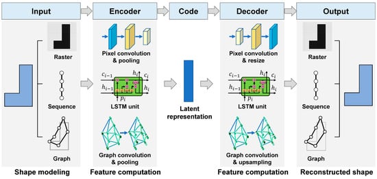
Figure 1.
Shape encoder–decoders designed for different data modeling of two-dimensional shapes.
2.1. Pixel-Based Shape Coding Model
The method of rasterization is commonly used to work with spatial vector-based data because regularized organization is better adapted to many algorithms or models [31], such as the deep convolutional neural networks. Another advantage of this approach is that the regional characteristics of the shapes are considered.
To obtain a raster-based image for a shape, the differences between the maximum and minimum values on the horizontal and vertical axes were calculated, and the larger value was taken as the edge length to obtain a square with the centroid of the shape considered as the center. This square was appropriately expanded outward (e.g., 10%) to ensure the integrity of the shape. A suitable grid was then established to rasterize the square. The size of the grid cells directly affects the clarity of the data content representation. If the cell size is too large, a serious mosaic phenomenon occurs, which makes it difficult to present the outline details. If the cell size is too small, the training efficiency of the model is affected. By considering the clarity of the images and the complexity of the model comprehensively, the grid size was set at 28 × 28 pixels in this study. Finally, the grid cell is binarized. That is, when a cell falls within the shape with more than half of the area, the cell is set to black; otherwise, it is white.
After converting the shape into a raster-based image, the classical encoder–decoder based on a grid-like topology can be used to extract the latent representation of the shape. Figure 2 shows the architecture of the pixel-based encoder–decoder (PixelNet) used in this study for shape encoding.
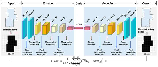
Figure 2.
Raster-based encoder–decoder model (PixelNet) for shape encoding.
The encoder in PixelNet encoded the input 28 × 28 image as a 128-dimensional vector. It contained three convolutional layers with a kernel size of 3 × 3 and kernel numbers of 3, 18, and 8, respectively. After each convolutional layer, a max-pooling layer with a window size of k = 2 × 2 and a stride length of s = 2 was connected. The decoder also contained three convolutional layers with 8, 18, and 3 kernels, respectively. The upsampling, the opposite of pooled sizing, restored the image to its original size. Finally, a convolutional layer with feature one was added to ensure that the feature dimension of the output was consistent with that of the input.
2.2. Sequence-Based Shape Encoding Model
The boundary of a shape is a natural sequence that comprises a series of contiguous points. Thus, constructing a shape representation and analysis framework based on the boundary sequence is a promising strategy.
Because the distance between two adjacent nodes on a shape boundary is not identical, the processing unit is not stationary. To address this issue, the boundary was divided into a series of consecutive linear units of equal lengths, termed lixels [32], and the midpoints of the lixels were considered as the sequence nodes. For each sequence node, the horizontal and vertical differences between the two ends of the associated lixel were used as the two features to describe it. Finally, a vector, , containing sequence nodes with two-dimensional features, was constructed to serve as the input for the shape encoding model. Referring the parameter settings used in the literature [3], was set to 64.
To process the constructed sequence, a neural network was used to construct an encoder–decoder. As the classical neural network does not consider the node orders in sequence, the Seq2seq network (SeqNet) [33], which uses long short-term memory (LSTM) [34] as the encoder and decoder, was adopted. The architecture is illustrated in Figure 3.
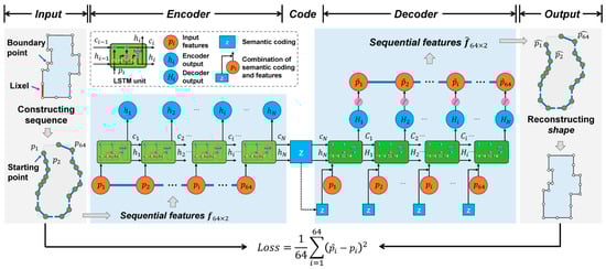
Figure 3.
Sequence-based encoder–decoder model (SeqNet) for shape encoding. For simplicity, the illustrated sequence does not show the actual number of nodes; however, the labels on the node number and dimensions are the actual values used in the model.
The encoder was an LSTM network that received the sequence as the input. The number of neurons in the hidden layer was set to , i.e., the encoding dimension of the input shape. The Tanh function was used to activate the neurons to ensure that each value of the output vector ranged from −1 to 1. The computation of each time step in the loop is as follows:
where and denote the output and state values of the LSTM unit, respectively, denotes the input features, and denotes the computation of each time step in the encoder. The output of the last time step is the shape encoding, i.e.,, where denotes the number of time steps.
The decoder consisted of an LSTM network and a fully connected layer. It received the combination of the intermediate shape encoding and the features as input, i.e., the input was an matrix. The number of hidden layer neurons was set to to maintain the same dimension as the state value in the encoder. The Tanh function was also used as an activation function. The output of the LSTM added a linear fully connected layer that constrained the dimension of the sequence output to the input dimension to reconstruct the original sequence. The computation process is as follows:
where and denote the output and state values of the LSTM unit, denotes the input for the decoder formed by the shape encoding and feature, denotes the computation of each time step in the decoder, and are the weights and biases of the fully connected layer, and is the feature reconstructed by the model.
The learning goal was to minimize the inputs, and the outputs, , and the difference was measured using the mean square error, computed as:
The decoder was trained through the ‘teacher-forcing’ approach to speed up the convergence of the model, i.e., each input of the decoder does not use the output of the previous time step but directly uses the value of the corresponding position in the training data.
2.3. Graph-Based Shape Autoencoder
Compared with the sequence, the graph can better express the relationship between nonadjacent nodes. A graph is mathematically denoted as , where and are the sets of nodes and edges connecting them, respectively, and is an adjacency matrix that records the edge weights. The Laplacian matrix of is computed as , where is the -order identity matrix and is the degree matrix composed of the degree of node . The eigenvectors of are denoted by , and the corresponding eigenvalues are . They satisfy , where is a matrix formed by , and is a diagonal matrix of .
In the same way that a sequence was constructed, the midpoints of lixels were considered as the graph nodes, and the horizontal and vertical differences between the two ends were used as the features of the graph nodes. To compute the edge weights, a Delaunay triangulation (DT) was constructed using all nodes. If a DT edge existed between two nodes, the weight of the edge connecting them was set as the reciprocal of the length of the DT edge; otherwise, it was 0. Finally, the graph node features matrix, , and the adjacency matrix, , were obtained to serve as inputs to the model. was also set to 64 to ensure that the node number and features are consistent with the SeqNet method for better comparison.
A graph-based encoder–decoder (GraphNet) was built to process the constructed graph. The overall architecture is illustrated in Figure 4. The encoder included one graph convolution layer with 32 feature maps (i.e., the number of kernels), and the polynomial order of each kernel was set to 3. It also contained two graph pooling layers. After pooling, the number of nodes and feature dimensions were set to 32 and 24 and 16 and 8, respectively. The output of the last layer in the encoder was expanded into a 128-dimensional feature vector, that is, the shape encoding. Correspondingly, there were two graph upsampling layers and one graph convolutional layer in the decoder to restore the size of the graph to be the same as the input.
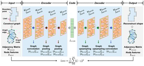
Figure 4.
Graph-based encoder–decoder model (GraphNet) for shape encoding. For simplicity, the illustrated graph does not show the actual number of nodes and features; however, the labels on the dimensions of the adjacency matrix and node features, as well as the convolution kernel parameters, are the actual values used in the model.
The convolutional layer was implemented by a fast and localized graph convolution operation, which was defined based on the graph Fourier transform [35]. The -th output features of the ()-th layer are computed by the layer-by-layer forward propagation rule:
where denotes a nonlinear activation function; is the graph of the layer; is K-order Chebyshev polynomial, which is recursively computed by , with and ; is the largest eigenvalue of ; and are the trainable coefficients and bias vector in the layer, respectively, and and are the number of graphs of the and layers, respectively.
The graph convolutional layer uses the Laplacian matrix to map the node features to . This process updates the graph node features, but it does not change the size of the graph (i.e., number of graph nodes). To this regard, the DIFFPOOL method [36] was used to implement the graph pooling and upsampling operations, which helps to change the graph size and extract hierarchical features. This layer learns a differentiable assignment matrix to map the nodes to the nodes to obtain node features with different granularities. It is implemented through two graph convolutions: and , where generates new node features, and generates the assignment matrix. The adjacency matrix and node features of the graph in the layer are computed as follows:
This process changes the number and features of the graph nodes. If is less than , it implies that the number of nodes is reduced, which can be understand as a pooling operation. Conversely, the number of nodes increases, that is, the upsapling operation.
The GraphNet was trained in an unsupervised manner to minimize the differences between the input and output. Considering the difficulty of optimizing the assignment matrices in the pooling layer, two constraints were added to the loss function [36]: minimizing the difference of the adjacent matrices for each layer and minimizing the entropy of the assignment matrices row by row. The former guarantees the stability of the edges in the adjacent matrices, and the latter guarantees that the assignment for each node is close to a one-hot vector to clearly describe the relationship with the next layer. The final loss function is defined as follows:
where is the number of all layers (i.e., six in this study), and and denote the Frobenius norm and entropy function, respectively.
3. Experimental Results and Analysis
The three deep encoder–decoders were implemented using Python in TensorFlow, and experiments on two datasets were conducted with an environment of Intel(R) Core (TM) i9-9920X CPU and NVIDIA GeForce RTX 2080Ti to test their performance for shape encoding. The following sections describe the experimental datasets, results, and analyses and provide a discussion.
3.1. Experimental Datasets
An open building shape dataset was used in the experiments [3]. As a typical artificial geographical feature, buildings are often represented in maps as two-dimensional shapes, with obvious visual features such as right-angle turns and symmetry. In this dataset, 10 categories of buildings were distinguished according to the forms of English letters, as shown in Figure 5. Each category contained 501 buildings, with a total of 5010 shapes.
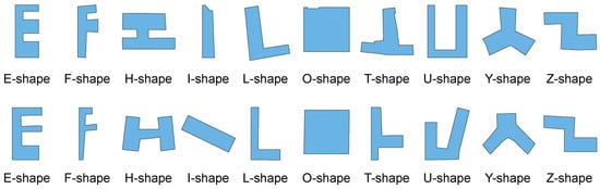
Figure 5.
Examples of the 10 categories of building shapes in the experimental dataset.
Because PixelNet, SeqNet, and GraphNet are all unsupervised models, the building dataset was not divided into training and test sets. All buildings were used to train the three models to eventually encode a one-dimensional vector for each building. The training batch size was set to 50, and each model was trained for 50 rounds using the Adam optimizer [37] with a learning rate of 0.01.
3.2. Experimental Results and Analysis
3.2.1. Quantitative Evaluation
Four shape retrieval metrics were used to evaluate the effectiveness of the shape encoding quantitatively: the nearest neighbor (NN), first tier (FT), second tier (ST), and discounted cumulative gain (DCG). All metrics range from 0 to 1, with a higher value indicating a better performance. For more information on the definitions and computation of these metrics, refer to the work of Shilane et al. [38].
To calculate FT, ST, and DCG, one shape was randomly selected from each category as the retrieval object and the others were the shapes to be retrieved. In addition, we also counted the average cost time of calculating the similarities between each retrieval object and other shapes to evaluate the retrieval efficiency of the models. For comparison, an existing graph-based deep learning model (GAE) proposed by Yan et al. [3] and two traditional methods, namely, the Fourier shape descriptor (FD) [9] and tangent function (TF) representation [19], were also implemented. The differences between the GAE and GraphNet methods are that GAE uses a sequence to represent the shape boundaries, while GraphNet uses a graph to model the shapes and integrates a pooling operation in the network. In addition, their input features are different. Table 1 lists the evaluation results of the shape retrieval on the building datasets.

Table 1.
Four quantitative evaluation metrics and cost time for the shape retrieval of the building dataset using different shape encoding methods.
Several observations were made through the comparison. First, GraphNet outperformed PixelNet and SeqNet for all four metrics in the building shape retrieval task. GraphNet not only considered the connections of non-adjacent nodes through a DT edge in the graph construction stage but also the spatial proximity between nodes using graph convolution. These considerations may be beneficial for capturing the contextual characteristics. Second, the overall performance of PixelNet was somewhere between those of the GraphNet and SeqNet models. This result proves that both the raster-based and vector-based methods are feasible for shape encoding. The raster-based method is simple and intuitive, whereas the vector-based method has the advantages of low redundancy, high precision, and being information intensive. For vector-based methods, the graph method is abler to mine the topological relationships between non-adjacent nodes than the sequence method. For this reason, although GraphNet and SeqNet methods have the same input features, GraphNet has displayed better shape coding capabilities than SeqNet for the building dataset.
Furthermore, compared with the traditional FD and TF methods, the four deep learning methods (GraphNet, PixelNet, SeqNet, and GAE methods) performed better. This result proves the effectiveness of deep learning technologies in extracting the implicit features of shapes and obtaining valuable encodings. In addition, by comparing the cost time, it was found that deep learning greatly improved the efficiency of shape retrieval. This is because the shape similarity measures obtained using the FD and TF methods are highly related to the starting point of the enclosed boundaries. For a more reliable retrieval, the similarity between two shapes was computed repeatedly by traversing all nodes in the boundaries as the starting point. This process incurs considerable computational cost. In contrast, deep learning provides only one encoding vector for each shape, with a very small computation when performing matching and retrieval.
3.2.2. Visualization Analysis
To demonstrate the performance of the shape encoding more intuitively, the t-SNE algorithm [39] was used to reduce the dimension of the shape encodings to two and visualize them in a plane space, as shown in Figure 6. Under ideal conditions, two shapes of the same category are more similar, their positions are closer in the space, and the positions of shapes with different categories are farther apart. Eventually, all building shape encodings form some independent clusters.
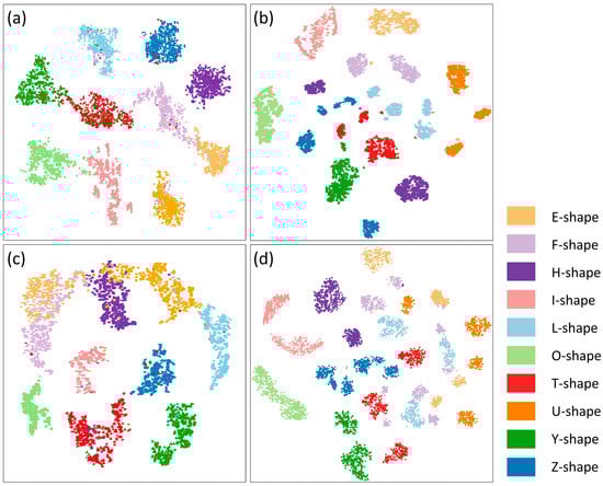
Figure 6.
Visualization of the building shape encodings produced by the four deep learning-based methods: (a) GraphNet, (b) SeqNet, (c) PixelNet, and (d) GAE. The same color indicates the same category.
From the results, the shape encodings produced by the four methods exhibited a certain aggregation phenomenon. A detailed comparison shows that the shape encodings produced by the GraphNet and PixelNet methods have a stronger aggregation, whereas the clusters formed by the same shapes in the SeqNet and GAE results show obvious separation. Analysis revealed that this phenomenon may be caused by the shape orientation and the starting point. Although the extracted features in the SeqNet and GAE methods are scalar, the node features of the input sequences vary greatly with the selection of the starting points. This leads to a significant difference in the shape encodings. In contrast, the separations of the shapes with the same category in the results of the GraphNet and PixelNet methods were mitigated greatly. This occurred because each shape was represented using a unified raster grid regardless of the choice of starting point in the PixelNet method. In the GraphNet method, this problem was effectively alleviated by considering the topological relationships between nodes. These separations resulted in non-negligible errors in the shape similarity measure, which may explain why the evaluation metrics of the SeqNet and GAE methods for the shape retrieval task were slightly lower than those of the GraphNet method.
Further, it was observed that there was overlap for some shape encodings in the GraphNet and PixelNet results. Especially, in the PixelNet result, E-shaped and F-shaped encodings have an obvious overlap. This phenomenon occurred may be because some shapes have a certain visual similarity, for example, the E-shape and F-shape were both rectangle-like and serrated. This overlap also led to errors in the shape similarity measure; therefore, the evaluation metrics of the PixelNet method for the shape retrieval task were inferior to those of the GraphNet method. From these two observations, the SeqNet and GAE methods are able to group shapes with the same starting point and orientation into a category. However, for the two shapes with different directions, these two methods may measure their similarity incorrectly. For the PixelNet and GraphNet methods, they are not affected by the orientation and starting points of the shapes, but they may not be able to distinguish some specific shapes sufficiently, especially for the PixelNet method.
3.2.3. Similarity Measurements between Shape Pairs
To explain the above results better, Table 2 lists the shape similarities between some typical shape pairs obtained using different methods. The similarity between two shapes was calculated using the Euclidean distance between their encodings. The smaller the value is, the more similar the two shapes are.
Table 2.
Shape similarities between some typical shape pairs using different methods. Red hollow dots indicate the starting point of the shapes, and small blue arrows indicate the node order.
For the first shape pair, the orientations, starting points, and overall shapes were relatively close, and all three methods could describe their similarities accurately. The orientations and starting points of the second shape pair were similar, but the shapes were different and the similarities computed by the three methods were low. The results show that the three methods can distinguish the shape features well under ideal conditions, i.e., with consistent orientations and starting points. The third shape pair has the same starting points and shapes, but the orientations are different, SeqNet performed well, GraphNet reasonably well, and PixelNet performed the worst. This result indicates that the orientation affected the performance of PixelNet observably; it also affected GraphNet to a certain extent but within an acceptable range. The results of the fourth and fifth shape pairs revealed that the SeqNet method always perform poorly when the starting points were different, even when the orientations were the same. This means that these methods are still very sensitive to the order of the points, even though the extracted features are scalar-free. This problem was significant alleviated in GraphNet. These detailed comparative analysis results are consistent with the previous quantitative results.
3.3. Discussions on the Coding Dimension
The encoding dimension variable is critical for the encoder–decoder method. Therefore, a supplemental experiment was conducted to investigate the effects of this parameter on the performance of the three methods. To achieve a change in dimensions, PixelNet and GraphNet adjusted the number of convolutional kernels in the last convolutional layer, and SeqNet adjusted the number of neurons in the hidden layer. Table 3 lists the evaluation metrics for the encoding performance of the different methods by varying the coding dimension from 32 to 512.
Table 3.
Quantitative evaluation results with four metrics for the shape retrieval of the building dataset using the three deep encoder–decoder methods with different encoding dimensions.
In theory, when the encoding dimension is higher, the feature representation ability is stronger. However, the experimental results contradicted this finding. The comparison revealed that the performance of all three methods first improved but then stabilized or even decreased as the encoding dimension increased. GraphNet performed the best when the encoding dimension was 128. For the PixelNet and SeqNet methods, the most appropriate encoding dimension was 256. This result may be attributable to the lack of sparsity in training to limit the base vector, resulting in performance degradation due to over-completeness at higher encoding dimensions.
3.4. Tests with a More Complex Dataset
Because the building shapes used in this study were relatively simple, we tested the different shape encoding methods on a more complex dataset, the MPEG-7 dataset [40], to verify and compare the performance further. This database is characterized by a wide variety of categories. It includes a total of 70 shape categories covering animals, plants, and supplies. Each category includes 20 shapes, for a total of 1400 shapes. Figure 7 shows some examples from the dataset.
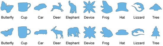
Figure 7.
Examples of shapes in the MPEG-7 dataset.
For the four deep learning models, all of the shapes in the MPEG-7 dataset were used to train them, and each shape was encoded as a vector. For each category, one shape was chosen randomly to retrieve the other shapes. The four quantitative metrics and the cost time of the retrieval task using different methods are listed in Table 4. The comparison shows that GraphNet still performed better on all four quantitative metrics compared with the PixelNet and SeqNet methods, and that the overall results are consistent with those for the building dataset, indicating that GraphNet also has a certain of advantages for the similarity measures and retrieval of complex shapes. The four metrics of the GAE method were still lower than the Graph method, but the gap had narrowed. Careful analysis revealed that the reason for this result may be that GAE had a simpler network architecture and received more input features, and therefore it performed more stably on the MPEG-7 dataset with complex categories and fewer shapes. It was also observed that, the metrics of FT and ST improved on the tests with the MPEG-7 dataset, especially for the FD and TF methods, which may be related to the reduction in the number of shapes in each category.
Table 4.
Four quantitative evaluation metrics and cost time for the shape retrieval of the MPEG-7 dataset using different shape encoding methods.
In addition, the cost time of the retrieval task for the four deep learning methods was shortened due to fewer retrieval objects in the dataset. The FD and TF methods, however, required more time because the shapes were more complex and the number of nodes were larger. This result further demonstrates the advantages of deep learning methods in terms of retrieval efficiency.
4. Conclusions
Shape representation and encoding is a foundational problem in cartography and geosciences. According to three basic modeling methods for shape, three different shape encoding methods based on deep learning, PixelNet, SeqNet, and GraphNet were constructed in this study. PixelNet was built on a raster-based modeling, SeqNet was built on a sequence-based modeling, and GraphNet was built on a vector-based modeling using a graph structure. Experimental analysis using two datasets produced the following conclusions: (1) The encoder–decoder methods based on deep learning could effectively compute the shape features and obtain meaningful encodings to support the shape measurement and retrieval task. (2) The deep learning methods demonstrated some advantages over the traditional FD and TF methods on the building dataset; the FT and ST metrics of FD and TF methods improved significantly on the MPEG-7 dataset. (3) GraphNet performed better than SeqNet and PixelNet due to its use of a graph to model the topological relations between nodes and an efficient graph convolution and pooling operation to process the node features.
Further research would be carried out from the following aspects: (1) The planar shape encoding problem should be extended to a three-dimensional (3D) shape encoding problem and the performance of encoder–decoders for encoding 3D objects, including 3D buildings and 3D points, should be evaluated. (2) For feature extraction of shape nodes, additional features deserve study to capture the morphology and topological associations between shape nodes, such as shape context descriptors. (3) In terms of learning architecture, some emerging learning techniques, such as attentional mechanisms and reinforcement learning, can be considered to enhance representation capability.
Author Contributions
Conceptualization, Xiongfeng Yan and Min Yang; methodology, Xiongfeng Yan; writing—original draft preparation, Xiongfeng Yan; writing—review and editing, Xiongfeng Yan and Min Yang; funding acquisition, Xiongfeng Yan and Min Yang. All authors have read and agreed to the published version of the manuscript.
Funding
This research was funded by the National Natural Science Foundation of China (Grant nos. 42001415, 42071450), the Open Research Fund Program of Key Laboratory of Digital Mapping and Land Information Application Engineering, Ministry of Natural Resources (Grant no. ZRZYBWD202101), and the State Key Laboratory of Geo-Information Engineering (Grant no. SKLGIE2020-Z-4-1).
Data Availability Statement
Data sharing is not applicable to this article as no new data were created in this study.
Conflicts of Interest
The authors declare no conflict of interest.
References
- Klettner, S. Affective communication of map symbols: A semantic differential analysis. ISPRS Int. J. Geo-Inf. 2020, 9, 289. [Google Scholar] [CrossRef]
- Klettner, S. Why shape matters—On the inherent qualities of geometric shapes for cartographic representations. ISPRS Int. J. Geo-Inf. 2019, 8, 217. [Google Scholar] [CrossRef]
- Yan, X.; Ai, T.; Yang, M.; Tong, X. Graph convolutional autoencoder model for the shape coding and cognition of buildings in maps. Int. J. Geogr. Inf. Sci. 2021, 35, 490–512. [Google Scholar] [CrossRef]
- Samsonov, T.E.; Yakimova, O.P. Shape-adaptive geometric simplification of heterogeneous line datasets. Int. J. Geogr. Inf. Sci. 2017, 31, 1485–1520. [Google Scholar] [CrossRef]
- Yan, X.; Ai, T.; Zhang, X. Template matching and simplification method for building features based on shape cognition. ISPRS Int. J. Geo-Inf. 2017, 6, 250. [Google Scholar] [CrossRef]
- Yang, M.; Yuan, T.; Yan, X.; Ai, T.; Jiang, C. A hybrid approach to building simplification with an evaluator from a backpropagation neural network. Int. J. Geogr. Inf. Sci. 2022, 36, 280–309. [Google Scholar] [CrossRef]
- Yan, X.; Ai, T.; Yang, M.; Yin, H. A graph convolutional neural network for classification of building patterns using spatial vector data. ISPRS J. Photogramm. Remote Sens. 2019, 150, 259–273. [Google Scholar] [CrossRef]
- Yang, M.; Jiang, C.; Yan, X.; Ai, T.; Cao, M.; Chen, W. Detecting interchanges in road networks using a graph convolutional network approach. Int. J. Geogr. Inf. Sci. 2022, 36, 1119–1139. [Google Scholar] [CrossRef]
- Ai, T.; Cheng, X.; Liu, P.; Yang, M. A shape analysis and template matching of building features by the Fourier transform method. Comput. Environ. Urban Syst. 2013, 41, 219–233. [Google Scholar] [CrossRef]
- Fan, H.; Zhao, Z.; Li, W. Towards measuring shape similarity of polygons based on multiscale features and grid context descriptors. ISPRS Int. J. Geo-Inf. 2021, 10, 279. [Google Scholar] [CrossRef]
- Belongie, S.; Malik, J.; Puzicha, J. Shape matching and object recognition using shape contexts. IEEE Trans. Pattern Anal. Mach. Intell. 2022, 24, 509–522. [Google Scholar] [CrossRef]
- Mark, D.M.; Freksa, C.; Hirtle, S.C.; Lloyd, R.; Tversky, B. Cognitive models of geographical space. Int. J. Geogr. Inf. Sci. 1999, 13, 747–774. [Google Scholar] [CrossRef]
- Basaraner, M.; Cetinkaya, S. Performance of shape indices and classification schemes for characterising perceptual shape complexity of building footprints in GIS. Inter. J. Geogr. Infor. Sci. 2017, 31, 1952–1977. [Google Scholar] [CrossRef]
- Wei, Z.; Guo, Q.; Wang, L.; Yan, F. On the spatial distribution of buildings for map generalization. Cartogr. Geogr. Infor. Sci. 2018, 45, 539–555. [Google Scholar] [CrossRef]
- Li, W.; Goodchild, M.F.; Church, R. An efficient measure of compactness for two-dimensional shapes and its application in regionalization problems. Int. J. Geogr. Inf. Sci. 2013, 27, 1227–1250. [Google Scholar] [CrossRef]
- Akgül, C.B.; Sankur, B.; Yemez, Y.; Schmitt, F. 3D model retrieval using probability density-based shape descriptors. IEEE Trans. Pattern Anal. Mach. Intell. 2009, 31, 1117–1133. [Google Scholar] [CrossRef]
- Kunttu, I.; Lepisto, L.; Rauhamaa, J.; Visa, A. Multiscale Fourier descriptor for shape-based image retrieval. In Proceedings of the 17th International Conference on Pattern Recognition, Cambridge, UK, 23–26 August 2004; pp. 765–768. [Google Scholar] [CrossRef]
- Sundar, H.; Silver, D.; Gagvani, N.; Dickinson, S. Skeleton based shape matching and retrieval. In Proceedings of the International Conference on Shape Modeling and Applications, Seoul, Korea, 12–15 May 2003; pp. 130–139. [Google Scholar] [CrossRef]
- Arkin, E.M.; Chew, L.P.; Huttenlocher, D.P.; Kedem, K.; Mitchell, J.S. An efficiently computable metric for comparing polygonal shapes. IEEE Trans. Pattern Anal. Mach. Intell. 1991, 13, 209–216. [Google Scholar] [CrossRef]
- Adamek, T.; O’connor, N.E. A multiscale representation method for nonrigid shapes with a single closed contour. IEEE Trans. Circuits Syst. Video Technol. 2004, 14, 742–753. [Google Scholar] [CrossRef]
- Yang, C.; Wei, H.; Yu, Q. A novel method for 2D nonrigid partial shape matching. Neurocomputing 2018, 275, 1160–1176. [Google Scholar] [CrossRef]
- Goodfellow, I.; Bengio, Y.; Courville, A. Deep Learning; The MIT Press: Cambridge, MA, USA, 2016; pp. 505–527. [Google Scholar]
- Bei, W.; Guo, M.; Huang, Y. A spatial adaptive algorithm framework for building pattern recognition using graph convolutional networks. Sensors 2019, 19, 5518. [Google Scholar] [CrossRef] [PubMed]
- Courtial, A.; El Ayedi, A.; Touya, G.; Zhang, X. Exploring the potential of deep learning segmentation for mountain roads generalisation. ISPRS Int. J. Geo-Inf. 2020, 9, 338. [Google Scholar] [CrossRef]
- Feng, Y.; Thiemann, F.; Sester, M. Learning cartographic building generalization with deep convolutional neural networks. ISPRS Int. J. Geo-Inf. 2019, 8, 258. [Google Scholar] [CrossRef]
- Zhu, D.; Cheng, X.; Zhang, F.; Yao, X.; Gao, Y.; Liu, Y. Spatial interpolation using conditional generative adversarial neural networks. Int. J. Geogr. Inf. Sci. 2020, 34, 735–758. [Google Scholar] [CrossRef]
- Ritter, S.; Barrett, D.G.; Santoro, A.; Botvinick, M.M. Cognitive psychology for deep neural networks: A shape bias case study. In Proceedings of the 34th International Conference on Machine Learning, Sydney, Australia, 6–11 August 2017; pp. 2940–2949. Available online: https://arxiv.org/abs/1706.08606 (accessed on 12 March 2022).
- Liu, C.; Hu, Y.; Li, Z.; Xu, J.; Han, Z.; Guo, J. TriangleConv: A deep point convolutional network for recognizing building shapes in map space. ISPRS Int. J. Geo-Inf. 2021, 10, 687. [Google Scholar] [CrossRef]
- Hu, Y.; Liu, C.; Li, Z.; Xu, J.; Han, Z.; Guo, J. Few-shot building footprint shape classification with relation network. ISPRS Int. J. Geo-Inf. 2022, 11, 311. [Google Scholar] [CrossRef]
- Courtial, A.; Touya, G.; Zhang, X. Representing vector geographic information as a tensor for deep learning based map generalisation. In Proceedings of the 25th AGILE Conference, Vilnius, Lithuania, 14–17 June 2022; p. 32. [Google Scholar] [CrossRef]
- Touya, G.; Zhang, X.; Lokhat, I. Is deep learning the new agent for map generalization? Int. J. Cartogr. 2019, 5, 142–157. [Google Scholar] [CrossRef]
- He, Y.; Ai, T.; Yu, W.; Zhang, X. A linear tessellation model to identify spatial pattern in urban street networks. Int. J. Geogr. Inf. Sci. 2017, 31, 1541–1561. [Google Scholar] [CrossRef]
- Sutskever, I.; Vinyals, O.; Le, Q.V. Sequence to sequence learning with neural networks. In Proceedings of the 27th International Conference on Neural Information Processing Systems, Montreal, QC, Canada, 8–13 December 2014; pp. 3844–3852. Available online: https://arxiv.org/abs/1409.3215 (accessed on 24 June 2022).
- Hochreiter, S.; Schmidhuber, J. Long short-term memory. Neural Comput. 1997, 9, 1735–1780. [Google Scholar] [CrossRef]
- Hammond, D.K.; Vandergheynst, P.; Gribonval, R. Wavelets on graphs via spectral graph theory. Appl. Comput. Harmon. Anal. 2011, 30, 129–150. [Google Scholar] [CrossRef]
- Ying, R.; You, J.; Morris, C.; Ren, X.; Hamilton, W.L.; Leskovec, J. Hierarchical graph representation learning with differentiable pooling. In Proceedings of the 32nd Conference on Neural Information Processing Systems, Montreal, QC, Canada, 3–8 December 2018; pp. 4805–4815. Available online: https://arxiv.org/abs/1806.08804 (accessed on 19 January 2022).
- Kingma, D.P.; Ba, J. Adam: A method for stochastic optimization. In Proceedings of the International Conference on Learning Representations (ICLR), San Diego, CA, USA, 7–9 May 2015; Available online: https://arxiv.org/abs/1412.6980 (accessed on 20 July 2022).
- Shilane, P.; Min, P.; Kazhdan, M.; Funkhouser, T. The Princeton shape benchmark. In Proceedings of the International Conference on Shape Modeling Applications, Genova, Italy, 7–9 June 2004; pp. 167–178. [Google Scholar] [CrossRef]
- Van der Maaten, L.; Hinton, G. Visualizing data using t-SNE. J. Mach. Learn. Res. 2008, 9, 2579–2605. Available online: http://jmlr.org/papers/v9/vandermaaten08a.html (accessed on 21 July 2022).
- Latecki, L.J.; Lakamper, R.; Eckhardt, T. Shape descriptors for non-rigid shapes with a single closed contour. In Proceedings of the Conference on Computer Vision and Pattern Recognition, Hilton Head, SC, USA, 13–15 June 2000; pp. 424–429. [Google Scholar] [CrossRef]


Publisher’s Note: MDPI stays neutral with regard to jurisdictional claims in published maps and institutional affiliations. |
© 2022 by the authors. Licensee MDPI, Basel, Switzerland. This article is an open access article distributed under the terms and conditions of the Creative Commons Attribution (CC BY) license (https://creativecommons.org/licenses/by/4.0/).