Identification and Mapping of High Nature Value Farmland in the Yellow River Delta Using Landsat-8 Multispectral Data

Abstract

The development of high nature value farmland (HNVf) can effectively improve the problems of biodiversity reduction, non-point source pollution and carbon loss in intensive farmland. To this end, we developed a set of general indicators based on Landsat 8 OLI imagery, including land cover (LC), normalized difference vegetation index (NDVI), Shannon diversity (SH) and Simpson’s index (SI). Combined with a Kohonen neural network (KNN), we assigned weights and developed the first potential HNVf map of the Yellow River Delta in China. The results showed that the four indicators were very effective for the expression of HNVf characteristics in the study area, and that SH and SI, in particular, could reflect the potential characteristics of HNVf at the edge of intensive farmland. LC, NDVI, SH and SI were weighted as 0.45, 0.25, 0.15 and 0.15, respectively. It was found that the potential HNVf type 2 (i.e., low-intensity agriculture, and natural and structural elements such as shrubs, woodlands and small rivers) in the study area was concentrated at the edges of intensive farmland, the transition zones from farmland to rivers and the estuary wetland areas of northern and eastern rivers. LC played a leading role in identifying HNVf. Based on six randomly selected real-world verification data from Map World, it was found that the accuracy of the validation set for HNVf type 2 was 83.33%, which exhibited the good development potential of HNVf in the study area. This is the first potential HNVf type 2 map of the Yellow River Delta in China and could provide a great deal of potential guidance for the development and protection of farmland biodiversity and regional carbon sequestration.

1. Introduction

High nature value farmland (HNVf) was proposed in the early 1990s as a new concept for a low-intensity agricultural system centered on biodiversity conservation [1,2]. At present, HNVf identification is widely carried out within the European Community (EC) and three clear types of farmland have been formed [3,4]: HNVf type 1 is farmland with a high proportion of semi-natural vegetation (i.e., shrubs, artificial linear forests, wetlands, small rivers, ecological ditches, wasteland with herbaceous plants, etc.) [1]; HNVf type 2 is farmland that contains natural and structural elements such as shrubs, woodlands, small rivers, or is dominated by low-intensity agriculture [1,4]; and HNVf type 3 is farmland that supports rare plant or animal populations [5]. The low-intensity properties of HNVf are important for soil carbon sequestration, cropland landscape heterogeneity and a high ecosystem carrying capacity.

Although HNVf has sustainable practical significance globally, current research on HNVf identification is limited to the EC. This is because reporting the extent and distribution of HNVf is mandatory for the European Union’s Rural Development Programme (RDP) in all member states [6]. However, the most important bottleneck is that there is not yet a complete set of quantitative reference indicators for the definition of HNVf. As a result, reports on HNVf identification outside the EC have yet to emerge.

Currently, the indicators for identifying HNVf mainly come from the CORINE Land Cover (CLC) database and the Integrated Administration and Control System (IACS) database, which are provided by the EC [7,8,9]. These databases contain land cover data and high-precision farm information (farm type, livestock, crops, etc.). Based on these databases, many scholars have developed terrain, soil quality and landscape indicators that can accurately infer the location and type of HNVf. For example, a list of CLC classes has been presented that could be used to identify HNVf [4]. Many scholars have also used IACS and LPIS data to evaluate the identification of HNVf and the annual changes in its range and distribution [10,11,12]. However, these databases have the shortcomings of low sample coverage and high restricted access, making it difficult to popularize them for use on a large scale. In addition, the high-resolution layer (HRL) small woody features (SWF), a new CLMS product, provides information on similar structures, such as linear hedges (https://land.copernicus.eu/, (accessed on 10 October 2022)). For example, the high-spatial-resolution SWF grid-aggregation layers can identify meaningful small woody features, especially in HNVf with obvious patches or linear features. However, these indicators only provide partial regional data within the EC and are not helpful for HNVf identification in other regions of the world.

In China, intensive farmland is being challenged by three key issues. The first issue is the reduction in farmland biodiversity. At least 60% of China’s arable land (cultivable non-agricultural land) is distributed in areas with a fragile ecological environment, which are very difficult to develop [13]. Most farmers have a low awareness of biodiversity conservation, and the over-exploitation of biological resources has led to its reduction and disappearance. These problems can cause biological disasters, including crop diseases and insect pests, and obviously also increase the ecological vulnerability of farmlands [14,15,16].

The second issue is the non-point source pollution of farmland. China has more than 20 million hectares of contaminated land [17]. He et al. (2017) found numerous soil pollution cases in China. This was mainly manifested in two aspects [18]: on the one hand, agricultural chemical fertilizers were subjected to short-term heavy rainfall and then overflow into water bodies, such as ditches, forming water bodies that were polluted with nitrogen and phosphorus eutrophication; on the other hand, pesticides, herbicides and some chemical fertilizers containing organophosphorus, organochlorine, microplastics and heavy metals can also cause non-point source water pollution [19,20,21,22].

The third issue is farmland carbon loss. In China, traditional farmland faces the challenge of carbon loss and human activities that lead to reductions in carbon storage within soil ecosystems [23,24]. The direct impact of this is unreasonable land use, such as deforestation, the drainage and agricultural use of natural wetlands, the conversion of grassland into farmland and reductions in soil carbon sequestration capacity [25,26]. The indirect impact is that human activities also change regional micro-climates. For example, climate warming causes extreme weather events, such as storms and heavy precipitation, which in turn cause carbon loss from farmland [27].

The development of HNVf is crucial to solving the above problems. In fact, much of the farmland in China is characterized by HNVf (including abandoned farmland). Since 2000, China has carried out a series of ecological projects, such as the returning farmland to lakes (RFL) campaign and the Grain for Green Program (GFGP). These measures to restore ecological diversity are more stringent than HNVf [28,29,30]. However, there are currently no standard HNVf indicators or datasets that are applicable to the Chinese region. Finding quantitative indicators for high nature value (HNV) that are suitable for the characteristics of Chinese farmland is very important for improving the above-mentioned problems of farmland biodiversity decline, non-point source pollution and carbon loss.

The purpose of our study was to determine whether indicators were useful in identifying potential characteristics of HNVf in China, such as land cover and landscape, which has never been explored before. Given the importance of and urgency for developing HNVf in China and the lack of regionally relevant datasets, in this study, we developed a set of minimally generic indicators that could be used to identify potential HNVf in China. In fact, there is existing HNVf in the eastern part of the study area: the “Shandong Yellow River Delta National Nature Reserve”, which was established in 1992 to protect the newborn wetland ecosystem and rare and endangered birds (http://hhsjzzrbhq.dongying.gov.cn/, (accessed on 20 May 2022)). According to the definition of HNVf type 3 (i.e., farmland that supports rare plant or animal populations), this nature reserve represents existing HNVf. However, we paid more attention to potential HNVf type 2 because it has the greatest development potential and could effectively improve the problems of reduced diversity, non-point source pollution and carbon loss in traditional Chinese farmland. Therefore, this study aimed to (i) apply identification indicators (i.e., land cover, normalized difference vegetation index, Shannon diversity, and Simpson’s index) in the Yellow River Delta region, (ii) build a Kohonen neural network (KNN) and develop high-resolution (30 m × 30 m) maps of potential HNVf type 2 and (iii) validate and evaluate the accuracy of the developed HNVf result using real-life data from Map World.

2. Materials and Methods

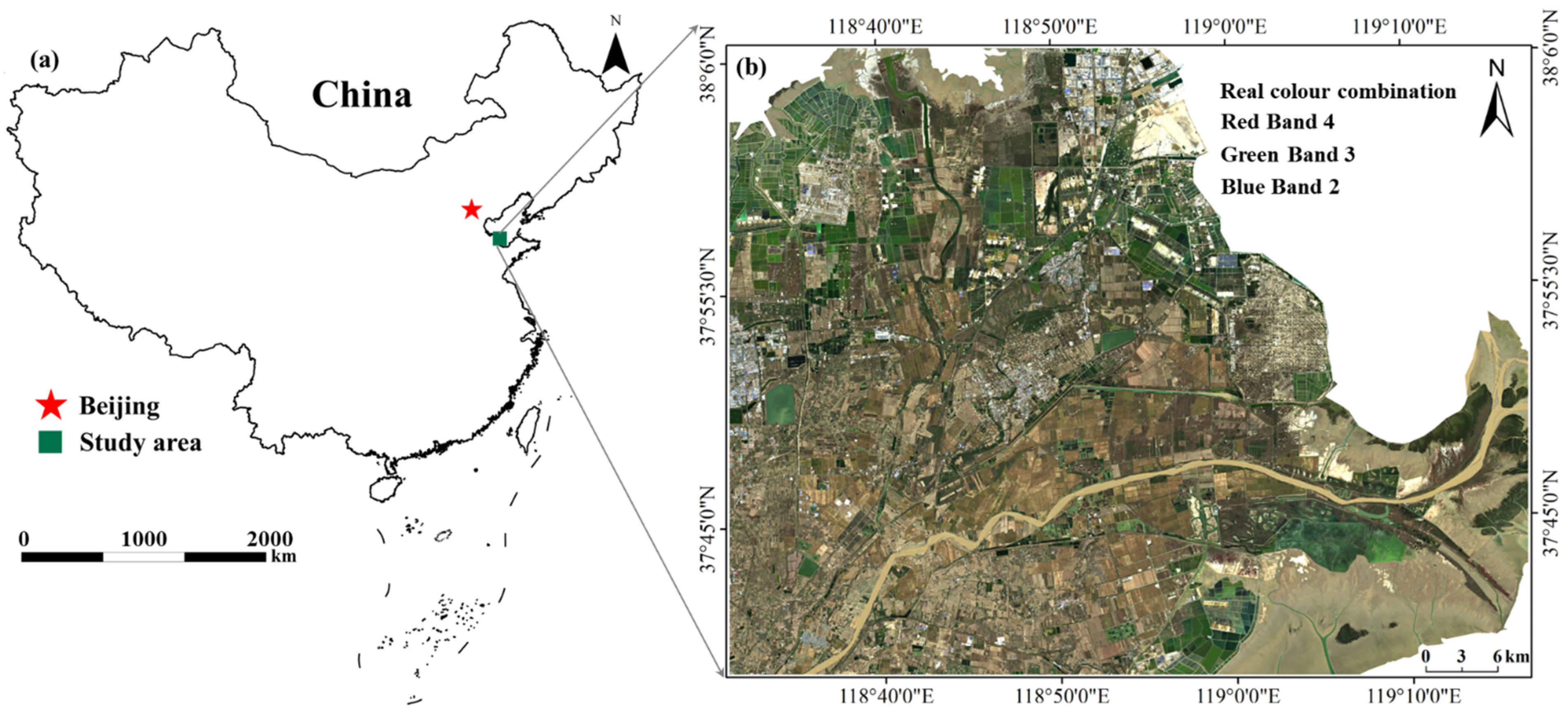
2.1. Study Area

The study area was located in the Yellow River Delta, China (37°40′ N–38°70′ N, 118°30′ E–119°20′ E) (Figure 1), which is in the continental monsoon climate temperate zone. According to public information from the Dongying statistical yearbook (http://www.dongying.gov.cn, (accessed on 10 January 2022)), the average annual temperature is 14.5 °C, the average annual precipitation is 628 mm and the annual average illumination is 2502.3 h. The elevation of the study area was close to sea level. The parent material of the soil in the area is impact loess. Intensive farmland is widely distributed along the river basin and the main crops include wheat, rice and corn. In 2021, the Central Committee of the Communist Party of China and the State Council issued the “Outline of Ecological Protection and High-Quality Development Plan for the Yellow River Basin” (http://www.gov.cn/zhengce/202110/08/content_5641438.htm, (accessed on 20 April 2022)), pointing out that it is necessary to restore the natural extension trend of the Yellow River Delta coastline, strengthen the protection of biological species in salt marshes, tidal flats and shallow estuarine wetlands, and explore the use of unconventional water sources to replenish bird habitats. In particular, farmland in the Yellow River Delta is facing challenges such as soil salinization and carbon loss. As a semi-natural agricultural system involving low-density farming and diverse land cover types, HNVf plays a key role in protecting regional biodiversity, restoring ecosystems and promoting sustainable agricultural development. Semi-natural vegetation is widely distributed across the Yellow River due to sedimentation in the Yellow River estuary and the serious salinization of the soil, so it is very suitable for the growth of salt and alkali-tolerant plants. This area is also very suitable for the development of HNVf, which plays an immeasurable positive role in promoting nitrogen and carbon circulation and inhibiting non-point source pollution.

2.2. Indicators

2.2.1. Land Cover Map

Land cover (LC) maps, as basic indicators to identify HNVf, play a crucial role in identification accuracy. This is because land cover types are proxy indicators of farming intensity [2,31]. In this study, we developed a land cover indicator with a resolution of 30 m, which was obtained using a Landsat 8 OLI image with a processing correction level of L1TP (10 November 2020), and data from the United States Geological Survey (USGS) server (https://earthexplorer.usgs.gov/, (accessed on 25 January 2022)). The OLI image was calibrated using radiation correction (i.e., applying FLAASH settings) and atmospheric correction (i.e., applying a FLAASH module) in ENVI 5.3 software (ESRI Inc., Redlands, CA, USA). Then, in order to obtain the optimal land cover map, four models (i.e., K-means, maximum likelihood, neural network, support vector machine) were selected for supervised classification in ENVI 5.3 software. The LC types were classified into five classes based on existing research [6]. The land cover map (30 m × 30 m) was finally obtained (Figure 2), including the following five LC types: built-up area (1), intensive farmland (2), woodland and grassland (3), water body (4) and semi-natural vegetation (5). Among these land cover types, water bodies included artificial reservoirs, salt fields and foreshores, while semi-natural vegetation mainly included shrubs, artificial linear forests, wetlands, small rivers, ecological ditches, wasteland with herbaceous plants, etc.

2.2.2. Vegetation Indicator

Vegetation cover is an essential element for HNVf mapping [32,33] that has been applied at local scales [34]. We selected the normalized difference vegetation index (NDVI) as a supplementary indicator to identify HNVf. Intensive farmland crops are harvested in December in northern China, so most farmland is in a state of bare soil. At this time, NDVI information mainly comes from woodland, bushes and wetland plants, effectively avoiding confusion with the spectral information of crops. This indicator was calculated based on the Landsat8 OLI image. The NDVI was obtained using the band calculation (Equation (1)) [35] for the OLI image after atmospheric correction, with a resolution of 30 m (Figure 3).

NDVI = (Band 5 − Band 4)/(Band 5 + Band 4)

(1)

2.2.3. Richness Indicator

Landscape indices express the socio-ecological dimension of systems; therefore, their structures and compositions can be used to identify HNVf [31,36]. HNVf largely overlaps with traditional agricultural landscapes, so landscape is also one of the essential characteristics of HNVf. We selected the Shannon diversity (SH) and Simpson’s index (SI) as indicators to characterize landscape heterogeneity, as they have been proven to be effective in identifying HNVf information [37]. SH accurately expresses the measure of variability (heterogeneity) in land cover within a small area and highlights the contribution formula of rare objects to the overall information (Equation (2)) (Figure 4). SI can be used as a comprehensive indicator to describe uniformity and richness, but is more inclined to the expression of uniformity (Equation (3)) [38,39] (Figure 5). Our calculations of SH and SI were implemented in Fragstats 4.2.1 software and we selected moving windows (neighborhoods) with a square side length 100 m in the analysis parameters module. In order to stay consistent with the value range of LC, the other indicators (i.e., NDVI, SH and SI) were normalized from 1 to 5 using a grid calculator and were then divided into five grades (non (1), low (2), moderate (3), high (4), and extremely high (5)) using the natural breakpoint method in ArcGIS 10.6 software.

$$\mathrm{SH}=-{\displaystyle \sum }_{\mathrm{i}=1}^{\mathrm{s}}{\mathrm{p}}_{\mathrm{i}}\ln {\mathrm{p}}_{\mathrm{i}}$$

(2)

$$\mathrm{SI}={\displaystyle \sum }_{\mathrm{I}=1}^{\mathrm{S}}{\mathrm{P}}_{\mathrm{i}}^2$$

(3)

where s is the total number of land cover types within the study area and p_i is the proportion of the i-th land cover type within the total area. When SH is equal to 0, it indicates that there is a single land cover type within the region [39].

In addition, in order to make the other factors consistent with LC, we normalized NDVI, SH and SI levels from 1 to 5. Each indicator was divided into five levels, and the higher the level, the higher the recognition potential for HNVf. The percentage of LC, NDVI, SH and SI pixels in each of the five levels was calculated. The pixel ratios of NDVI, SH and SI in the five levels of LC (i.e., built-up areas, intensive farmland, woodland and grassland, water bodies, and semi-natural vegetation) were also calculated. Furthermore, the pixels of the different indicators at the five levels were calculated from the HNVf map and the response relationships between HNVf and LC, NDVI, SH and SI were obtained with statistical analysis.

2.2.4. Weight Determination Method

Kohonen neural networks (KNNs) are a self-organizing neural feature mapping model that were first proposed in 1980 and are based on the research results from physiology and brain science [40,41,42,43]. Nerve cells in the human brain are arranged in an orderly way within a two-dimensional space and there is lateral interaction between nerve cells in adjacent areas, which leads to the emergence of inter-cell competition. KNNs simulate these characteristics and the working mechanism, classifying data based on a clustering analysis algorithm [44,45,46]. In this study, we paid more attention to the importance contribution of the four indicators in the clustering process. Then, the importance contribution of each indicator was set as its weight, which was very effective for constructing the weights of the identification indicators.

The steps of our KNN algorithm were as follows: (1) input the sample data into the neural network and calculate the distance between the input node and the output node; (2) obtain the winning neuron through a competition among the neurons in the competition layer; (3) adjust the weights of the input data and repeatedly train the network according to the above process until all samples have corresponding winning neurons and the competition is over; (4) correlate all data according to the final weights and divide them into different categories. In this study, a KNN was used to calculate the weights of identification indicators to avoid the subjectivity of prior knowledge weighting and we introduced a competition mechanism that could effectively improve the clustering accuracy. The KNN model was developed using SPSS modeler 18.0 software (IBM Inc., Armonk, NY, USA). Random points were generated within the study area, and the gradients of the random points were set as 500, 1000, 2000, 4000, 6000, 8000 and 10,000. The corresponding values of the LC, NDVI, SH and SI pixels were extracted using these random points, and then the Kohonen model was constructed with four clusters.

2.2.5. Validation of HNVf Identification Results

So far, not many studies have verified or analyzed HNVf identification results, which is due to the lack of real verification data. Therefore, it is difficult to obtain high-resolution real-life images of HNVf recognition patches on a regional scale. Using real maps (such as from Google Maps) has been proven to be very effective for verifying HNVf maps [7]. In this study, real-life data from Map World (https://www.tianditu.gov.cn/, (accessed on 11 September 2022)) and field surveys were used for validation purposes. Map World is a comprehensive geographic information service website that was built by the National Administration of Surveying, Mapping and Geoinformation, which provides 2.5 m resolution satellite remote sensing images nationwide. We randomly selected six verification areas within our HNVf map, compared the real map to the selected HNVf patches, and verified whether the HNVf identification result was accurate.

3. Results

3.1. Supervised Classification of Land Cover Types

Compared to other models, the SVM had the highest classification accuracy (94.77%) and Kappa coefficient (0.9027) (

Table 1. Classification accuracy of land cover types with different models.

Classification Method	Overall Accuracy (Kappa Coefficient)
Maximum likelihood	82.49% (0.7987)
Neural network	87.26% (0.8495)
Support vector machine	94.77% (0.9027)
K-means	71.19% (0.5724)

) and exhibited powerful performance for identification of land cover types. Furthermore, the classification accuracy for each LC type is shown in

Table 2. Accuracy evaluation of each land cover type in SVM model.

Accuracy Evaluation	Intensive Farmland	Woodland and Grassland	Built-Up Areas	Semi-Natural Vegetation	Water Body	Overall Accuracy (Kappa Coefficient)
Commission	1.72	17.75	8.69	12.74	1.11	94.77% (0.9027)
Omission	5.48	5.88	13.56	6.79	4.48
Producer accuracy	94.52	94.12	86.44	93.21	95.52
User accuracy	98.28	82.25	91.31	87.26	98.89

. Water body and intensive farmland had the lower commission (1.11% and 1.72%) and the highest user accuracy (98.89% and 98.28%) in comparison with other land cover types.

3.2. Statistical Analysis

The percentage of LC, SH and SI pixels in levels 1 and 2 was more than 60% (Figure 6a), which indicated that the classification could effectively eliminate non-HNVf pixels (i.e., built-up areas and intensive farmland). However, NDVI pixels were distributed above level 3, and the low-level vegetation images were very small. The pixel distributions of SI and SH were similar and the pixel proportion of SI in levels 4 and 5 was higher than that of the other factors (35.59%). In addition, the spatial correlation analysis of the four factors (Figure 6b) showed that LC was negatively correlated with NDVI (−0.77), SH (−0.67) and SI (−0.65). The positive correlation between SI and SH was high (0.89), and the correlation between NDVI and SH (0.046) and NDVI and SI (0.039) was low.

On the whole, from L1 to L5 of the LC types, the proportions of the other factors gradually decreased, which was due to the scarcer distribution of semi-natural vegetation (L5) and small rivers (L4) (Figure 6c). Among them, SH and SI accounted for the highest proportion in intensive farmland areas (L1), especially in level 4 (SHlc4 and SIlc4) pixels of intensive farmland (L1) areas, where they accounted for 85.45% and 76.58% respectively, and the fifth level (SHlc5 and SIlc5) pixels accounted for 76.88% and 71.03%, respectively.

3.3. Weight Calculation

Figure 7a shows the changes in each indicator’s weight under the different point gradients. For example, the four-colored band widths became thinner from left to right (i.e., the importance contribution value decreased) in P500. The four bands of the same color in Figure 7a correspond to the LC, NDVI, SH and SI indicators. In other words, the total importance of the four indicators in the KNN modelling results for P500 was 1 and the importance contributions of LC, NDVI, SH and SI were 0.43, 0.29, 0.14 and 0.15, respectively. When the number of random points was more than 4000, the weights of LC, NDVI, SH and SI became stable. The importance contributions of LC and NDVI fluctuated around 0.45 and 0.25, respectively. The weight of LC was set as 0.45, which was similar to the weight distribution results in other studies. For example, semi-natural habitat cover was used as a direct indicator of HNVf and was set to the maximum weight (0.45) [4,47]. NDVI could reflect certain characteristics well, such as hedgerows, grass slopes and tree lines, within field boundaries, with a weight of 0.25. SH and SI were related to the high level of semi-natural habitat and species diversity, and were as important as the characteristics of field boundaries, with a weight of 0.15.

3.4. HNVf Map

According to the weights of the indicators, a HNVf identification map with five levels was obtained using weighted superposition. White and light green represented non-agricultural areas (i.e., built-up areas) and intensive farmland areas, respectively, and any green area (above level 3) can be considered to have the possibility of being HNVf. It can be seen that with an increase in level, semi-natural habitat land cover also increased (Figure 7b). SH and SI showed a downward trend from grade 3 to 5, and the scores of these two indicators were highest in grade 3 (59.80% and 48.77%, respectively). NDVI accounted for the highest proportion of pixels in grade 4 (56.44%), while land cover was the highest in grade 5 (53.48%), indicating that semi-natural vegetation LC played a key characterization role for HNVf mapping. Based on the identified HNVf results (Figure 8), farmland in grades 3 and 4 within the study area was mainly distributed in the edges and transition zones of intensive farmland, and farmland in grade 5 was distributed around the estuaries of rivers in the north and east.

In the remote sensing image in Figure 9, the dark green area contains HNVf elements, such as trees, shrubs, grassland and small rivers, while the light brown area mainly includes intensive farmland, bare land, and the Yellow River. Among these verification regions, the proportion of HNVf elements in the five regions was high (more than 70%) (Figure 9a,b,d–f), indicating that these regions had great potential for HNVf. The proportion of HNVf elements in Figure 9c was relatively low (about 50%). Very low proportions of HNVf elements (less than 20%) did not exist in any of the verification regions and they all had grade 4 or 5 HNVf characteristics. On the whole, the accuracy of the validation set conforming to the HNVf type 2 was 83.33%.

In the validation areas, most of the was distributed along farmland edges (Figure 9c–e), which could be identified as transitional landscapes between forests and farmland. These landscapes included linear forests, grasslands, rivers and some intensive farmland, and had obvious high-intensity HNVf type 2 characteristics. In Figure 9a,b, these areas were identified as having a high proportion of natural vegetation landscapes, which included forests, shrubs, grasslands and rivers. Only sporadic fields were distributed among these exceptionally HNV areas, which exhibited an obvious potential for HNVf. The dominant HNVf area within the study area was type 2 (i.e., at the edge of intensive farmland) and the transitional landscape between forests and small rivers was distributed around almost all cities in the region. The validation accuracy of the real Map World data was high, which showed that the study area had great potential for HNVf. In addition, one region had a low number of HNVf characteristics and was significantly affected by intensive farmland (Figure 9c), and one region (Figure 9f) did not contain any intensive farmland, all of which belonged to high potential HNVf. However, this region belongs to the Yellow River Delta Nature Reserve (i.e., HNVf type 3), which was confused with HNVf type 2 in this study.

In addition, we conducted a field survey based on potential HNVf patches (Figure 10). Figure 10a shows that the high potential HNVf feature regions did contain linear forests, shrubs, grasslands and other HNVf feature elements. These HNVf patches exhibited significant differences with intensive farmland (Figure 10b). Field research is a reliable verification method, but it requires high human and financial costs, so it is recommended as a supplementary way to accurately identify HNVf patches based on verification results of real-life data from high-resolution remote sensing images.

4. Discussion

4.1. Potential Effect of Identification Indicators

Results of the SVM were similar with other studies for the classification of land cover types [48,49]. The possible reason for the high accuracy of water body identification was the small area ratio for this land cover type in the study region, and there were fewer confusion patches of wetland waters in the dry season. Moreover, the reduced vegetation cover in winter may be a cause of the low identification accuracy of woodland and grassland. This is because many plants in northern China are withered in the winter, resulting in insufficient vegetation information. However, this is why vegetation information regarding HNVf for some land covers, such as woodland and shrubs, can be well preserved. In short, the classification accuracy of the SVM model for the land cover map could satisfactorily identify HNVf features.

The results of pixel distributions of all indicators indicated that SH and SI were very effective for the expression of potential HNVf characteristics at intensive farmland edge and transition zones. The proportion of NDVI (NDVIlc1–NDVIlc5) in the woodland and grassland (L3) LC was very high, which further demonstrated that the HNVf feature information from trees and shrubs was very detailed when using NDVI during the winter. The proportion of NDVI, SH and SI in the woodland and grassland, water bodies and semi-natural vegetation (i.e., L3, L4, and L5) LC types were low because the number of patches of these three LC types was small, meaning the number of pixels extracted from the other factors was also small. On the whole, these indicators were effective for the representation of farmland edges and transition zones and had great potential for identifying HNVf type 2 in the study area.

4.2. Distribution of HNVf

We found that most of the nature reserves overlapped with high-intensity HNVf (Figure 9f). That is, there was some confusion between the HNVf type 2 identified in this study and the nature reserves (HNVf type 3). This was due to a large part of the nature reserve being defined as non-cultivated land (i.e., large areas of natural forest, wetlands and habitats for rare species). However, it also provided a new idea for identifying HNVf type 3 regions. At present, there is no special research to identify HNVf type 3, which mostly comprises rare animal and plant habitats, and it is necessary to accurately identify these areas in combination with the remarkable living habits of the animals and plants. However, these living habits were difficult to quantify. Based on the identification results for HNVf type 2, it could be possible to accurately identify the habitat range of rare animals and plants using feature extraction and feature quantification. For example, many studies have added biological, environmental, and agricultural data to HNVf maps, which could be regarded as “the definition of HNVf” [31,50,51].

The selected identification indicators for HNVf in this study were basically consistent with those in previous studies, and many scholars had introduced many innovative indicators to identify the characteristics suitable for their own countries or research areas. Our selected indicators reflected the principle of easy access and strong representativeness, in order to make up for the gap in HNVf research in China. Much research has focused on the identification of HNVf type 2 because it is more difficult to identify accurately. Actually, HNVf type 2 is more of a “transition” between HNVf type 1 and HNVf type 3. HNVf type 1 comprises semi-natural vegetation that is easy to identify, and many scholars have used semi-natural vegetation as an important basis for HNVf identification [6,7]. In fact, semi-natural vegetation is also one of the main features of HNVf and is an important indicator of whether patches have the potential of HNVf type 1. However, HNVf type 3 is difficult to quantify [52]. For example, due to the lack of indicators that correspond to HNVf type 3, the elements of HNV type 3 (such as breeding areas for geese and swans) have been added to HNVf maps in combination with NPWS priority agricultural environment areas (priority areas are based on the species and habitats in agricultural areas that have high natural protection value, which are beyond designated special protection areas) so as to obtain optimal estimations for the range and distribution of HNVf [6]. In fact, this overlapping phenomenon between different types of HNVf can be modeled using higher resolution data to distinguish HNVf type 2 and HNVf type 3.

4.3. Uncertainty of HNVf Identification

The uncertainty of multiple indicators is a key reason for confusion in HNVf maps, so the uncertainty caused by indicators should be considered in the interpretation of results. In this study, although the verification accuracy of the identification result was high, it is worth noting that there could still be some unidentified HNVf regions in the non-HNVf areas. Conversely, there could be some unidentified non-HNVf regions in the HNVf areas. This identification method was based on multi-source indicators, so there was inevitably some uncertainty related to the HNVf map, especially in terms of the scale effects of the indicators. For the same region, the spatial resolution of the indices significantly affected the feature responses of HNVf elements. This has also been reflected in some other studies [6,53], so the uncertainty of HNVf maps may come from the availability of input indicators with different spatial resolutions [31]. If the spatial resolution of the indicator is improved, then the identification accuracy may be improved; for example, if the discrimination of semi-natural vegetation is improved, then the identification accuracy for hedgerows and woodland could be higher. In addition, improved spatial resolutions for habitat mapping (e.g., high-resolution remote sensing) are highly likely to affect the HNVf output accuracy [6]. However, high-spatial-resolution indicators are currently very difficult to obtain. There has been no research into the identification of HNVf using different spatial resolutions, and we hope to discuss this in detail in subsequent studies. Moreover, the practicability and effectiveness of high-spatial-resolution indicators that can accurately distinguish between HNVf type 2 and HNVf type 3 need to be evaluated. Some characteristics of rare animal habitats in HNVf type 3 areas may be identified using ultra-high-resolution images from an unstaffed aerial vehicle (UAV).

Spatial resolution significantly affected the uncertainty of HNVf identification results. The uncertainty of identification results caused by the low spatial resolution of land cover has become a widespread consensus [31]. Most methods are based on land cover products, and the resolution of these products is often too low to fully determine the finer landscape features that may contribute to overall biodiversity [37]. At present, land cover maps with resolutions from 1 km to 100 m are used to identify HNVf (

Table 3. Spatial resolution of land cover maps for HNVf identification.

Study Area	Resolution	Land Cover Types	HNVf Identification Result	Reference
Ireland	2 km × 2 km	Beach, water, pasture, arable land, shrubs	The most comprehensive method for identifying HNVf.	[6]
Italy	50 m × 50 m	Urban areas, arable land, permanent crops, pastures and heterogeneous agricultural areas, forests, semi-natural areas, wetlands and water bodies	Compared to traditional land cover maps, agricultural statistics improved the identification results for HNVf.	[7]
Estonia	1 k m × 1 km	Inland plots, coastline intersection or contact plots, urban areas	The distribution of exceptional HNV, median HNV and relatively low nature value in 1 km squares was identified.	[51]
Italy	100 m × 100 m	Farmland, non-irrigation arable crops	A potential method to better identify HNVf type 3.	[54]
Wales	1 km × 1 km	Grassland, arable and horticultural land, coniferous woodland, urban areas	HNVf type 1 was identified using semi-natural vegetation.	[55]
French	1 km × 1 km	Semi-natural elements, urban areas, agricultural areas	Indicators from the HNV, HANPP framework and IC/ha were complementary to each other.	[56]

). It has been found that the higher the spatial resolution of a land cover map, the more accurate the identification results. For example, the third type of HNVf can be better identified using 100 m resolution images of farmland (non-irrigation arable crops) [54]. Single pixel coverage areas of HNVf that are identified by low resolution indices are large, so the expression of HNVf type 2 in transition zones is not effective. The possibility of mixing pixels from intensive farmland is higher. Although the recognition accuracy of high-resolution indices may be improved, it is difficult to obtain high-resolution verification images. UAV aerial images may be an effective verification method. In addition, this study proposes a set of minimum common indicators for identifying high-potential HNVf in plain areas. In order to achieve accurate identification of HNVf in different regions, the terrain, soil, climate, biological species and other elements need to be considered. For example, in central and western China, topographic relief and differences of climatic conditions caused by vegetation cover will significantly affect the distribution of HNVf, and the impact of these factors should be considered.

Specifically, we believe that HNVf results from the same region that are identified using different spatial resolution indicators may demonstrate a spatial drift characteristic. HNVf results identified using indicators with different resolutions in the same region may move within superposition space (i.e., demonstrate a drift phenomenon). In other words, assuming that the distribution of HNVf within the same region is highly homogenous, the differences between HNVf results identified using high-resolution and low-resolution indicators would be relatively small. The distribution of HNVf in high-resolution and low-resolution results can be approximately regarded as inclusion superposition. On the contrary, if the heterogeneity is very high, the difference between HNVf results identified using high-resolution and low-resolution indicators would increase sharply. Then, the identification results for HNVf from high-resolution indicators may appear in the non-agricultural regions of identification results from low-resolution indicators, or the HNVf results identified using low-resolution indicators may appear in the non-agricultural region of the identification result with the high-resolution indicator. This could lead to remarkable spatial drift characteristics. Therefore, exploring the scale effect of different spatial-resolution indicators within the same region could help to develop more accurate HNVf maps.

This is the first HNVf map of the Yellow River Delta in China to identify the possible distribution of HNVf based on objective indicators. However, in order to achieve an accurate identification of HNVf in different regions of China, the terrain, soil, climate, biological species and other indicators need to be further considered. For example, in central and western China, topographic relief and climatic conditions caused by vegetation cover could significantly affect the distribution of HNVf, so the impact of these factors should be considered. We believe that when identifying HNVf in other regions of China, considering indicators for the regional characteristics on the basis of the indicators used in this study could help to identify HNVf more accurately. Although there are some confusions between HNVf type 2 and HNVf type 3 on our map, it could still provide a great deal of potential guidance for the development and protection of farmland biodiversity and carbon sequestration in regional HNVf areas in China. In future research, we aim to further explore the scale effects of indicators and quantify the spatial drift characteristics of HNVf maps based on multi-source indicators at different scales to achieve more accurate evaluations.

5. Conclusions

In this paper, we developed LC, NDVI, SH and SI indicators to identify the first potential HNVf type 2 map of the Yellow River Delta, China. The characteristics of HNVf type 2 in the study area were concentrated around intensive farmland and transition zones to rivers. These indicators demonstrated immeasurable potential for identifying HNVf type 2 in the study area; in particular, SH and SI were very effective for the expression of potential HNVf characteristics at the edges and transition zones of intensive farmland. In addition, using Map World images effectively verified our HNVf map. Furthermore, the spatial resolution of the identification indicators significantly affected the spatial responses of HNVf characteristics. In the future, spatial changes in the identification indicators under different spatial resolutions should be compared to overcome the spatial drift phenomenon of HNVf maps.

References

1. Andersen, E.; Baldock, D.; Brouwer, F.M.; Elbersen, B.S.; Godeschalk, F.E.; Nieuwenhuizen, W.; van Eupen, M.; Hennekens, S.M. Developing a High Nature Value Farming Area Indicator; EEA: Copenhagen, Denmark, 2004; pp. 9–12. [Google Scholar]
2. Beaufoy, G.; Baldock, D.; Clarke, J. The Nature of Farming e Low Intensity Farming Systems in Nine European Countries; IEEP: London, UK, 1994; p. 68. [Google Scholar]
3. Keenleyside, C.; Beaufoy, G.; Tucker, G.; Jones, G. High nature value farming throughout eu-27 and its financial support under the cap. Inst. Eur. Environ. Policy Lond. 2014, 10, 91086. [Google Scholar]
4. Paracchini, M.L.; Petersen, J.; Hoogeveen, Y.; Bamps, C.; Burfield, I.; van Swaay, C. High Nature Value Farmland in Europe. An Estimate of the Distribution Patterns on the Basis of Land Cover and Biodiversity Data; Office for Official Publications of the European Communities: Luxembourg, 2008; p. 23480. [Google Scholar]
5. IEEP. Guidance Document to the Member States on the Application of the High Nature Value Indicator; IEEP: London, UK, 2007. [Google Scholar]
6. Matin, S.; Sullivan, C.A.; Finn, J.A.; Green, S.; Meredith, D.; Moran, J. Assessing the distribution and extent of high nature value farmland in the republic of Ireland. Ecol. Indic. 2020, 108, 105700. [Google Scholar] [CrossRef]
7. Bonato, M.; Cian, F.; Giupponi, C. Combining LULC data and agricultural statistics for a better identification and mapping of high nature value farmland: A case study in the Veneto plain, Italy. Land Use Policy 2019, 83, 488–504. [Google Scholar] [CrossRef]
8. EEC. Council Regulation (EEC) No 3508/92 of 27 November 1992 establishing an integrated administration and control system for certain Community aid schemes. Off. J. L 1992, 46, 0001–0005. [Google Scholar]
9. Steinmann, H.; Dobers, E.S. Spatio-temporal analysis of crop rotations and crop sequence patterns in northern Germany: Potential implications on plant health and crop protection. J. Plant Dis. Prot. 2013, 120, 85–94. [Google Scholar] [CrossRef]
10. Nitsch, H.; Osterburg, B.; Roggendorf, W.; Laggner, B. Cross compliance and the protection of grassland—Illustrative analyses of land use transitions between permanent grassland and arable land in German regions. Land Use Policy 2012, 29, 440–448. [Google Scholar] [CrossRef]
11. Ribeiro, P.F.; Santos, J.L.; Bugalho, M.N.; Santana, J.; Reino, L.; Beja, P.; Moreira, F. Modelling farming system dynamics in high nature value farmland under policy change. Agric. Ecosyst. Environ. 2014, 183, 138–144. [Google Scholar] [CrossRef]
12. Bartel, A.; Süßenbacher, E.; Sedy, K. “High Nature Value Farmland” für Österreich-Weiterentwicklung Des Indikators; Umwelt Bundesamt Wien: Dessau-Roßlau, Germany, 2011. [Google Scholar]
13. Penghui, J.; Manchun, L.; Liang, C. Dynamic response of agricultural productivity to landscape structure changes and its policy implications of Chinese farmland conservation. Resour. Conserv. Recycl. 2020, 156, 104724. [Google Scholar] [CrossRef]
14. Wang, H.; Zhang, C.; Yao, X.; Yun, W.; Ma, J.; Gao, L.; Li, P. Scenario simulation of the tradeoff between ecological land and farmland in black soil region of northeast China. Land Use Policy 2022, 114, 105991. [Google Scholar]
15. Flandroy, L.; Poutahidis, T.; Berg, G.; Clarke, G.; Dao, M.; Decaestecker, E.; Furman, E.; Haahtela, T.; Massart, S.; Plovier, H. The impact of human activities and lifestyles on the interlinked microbiota and health of humans and of ecosystems. Sci. Total Environ. 2018, 627, 1018–1038. [Google Scholar] [CrossRef]
16. Xu, D.; Li, D. Variation of wind erosion and its response to ecological programs in northern China in the period 1981–2015. Land Use Policy 2020, 99, 104871. [Google Scholar]
17. Hu, H.; Jin, Q.; Kavan, P. A study of heavy metal pollution in China: Current status, pollution-control policies and countermeasures. Sustainability 2014, 6, 5820–5838. [Google Scholar] [CrossRef] [Green Version]
18. He, K.; Sun, Z.; Hu, Y.; Zeng, X.; Yu, Z.; Cheng, H. Comparison of soil heavy metal pollution caused by e-waste recycling activities and traditional industrial operations. Environ. Sci. Pollut. Res. 2017, 24, 9387–9398. [Google Scholar] [CrossRef]
19. Ren, S.; Song, C.; Ye, S.; Cheng, C.; Gao, P. The spatiotemporal variation in heavy metals in China’s farmland soil over the past 20 years: A meta-analysis. Sci. Total Environ. 2022, 806, 150322. [Google Scholar]
20. Zhang, Q.; Wang, Y.; Jiang, X.; Xu, H.; Luo, Y.; Long, T.; Li, J.; Xing, L. Spatial occurrence and composition profile of organophosphate esters (opes) in farmland soils from different regions of China: Implications for human exposure. Environ. Pollut. 2021, 276, 116729. [Google Scholar] [CrossRef] [PubMed]
21. Liu, M.; Jia, Y.; Cui, Z.; Lu, Z.; Zhang, W.; Liu, K.; Shuai, L.; Shi, L.; Ke, R.; Lou, Y. Occurrence and potential sources of polyhalogenated carbazoles in farmland soils from the three northeast provinces, China. Sci. Total Environ. 2021, 799, 149459. [Google Scholar] [CrossRef]
22. Hu, J.; He, D.; Zhang, X.; Li, X.; Chen, Y.; Wei, G.; Zhang, Y.; Ok, Y.S.; Luo, Y. National-scale distribution of micro (meso) plastics in farmland soils across China: Implications for environmental impacts. J. Hazard. Mater. 2022, 424, 127283. [Google Scholar] [CrossRef]
23. Zhang, X.; Chen, S.; Yang, Y.; Wang, Q.; Wu, Y.; Zhou, Z.; Wang, H.; Wang, W. Shelterbelt farmland-afforestation induced soc accrual with higher temperature stability: Cross-sites 1 m soil profiles analysis in NE China. Sci. Total Environ. 2022, 814, 151942. [Google Scholar]
24. Song, X.; Yang, F.; Wu, H.; Zhang, J.; Li, D.; Liu, F.; Zhao, Y.; Yang, J.; Ju, B.; Cai, C. Significant loss of soil inorganic carbon at the continental scale. Natl. Sci. Rev. 2022, 9, b120. [Google Scholar] [CrossRef]
25. Zhu, G.; Shangguan, Z.; Hu, X.; Deng, L. Effects of land use changes on soil organic carbon, nitrogen and their losses in a typical watershed of the loess plateau, China. Ecol. Indic. 2021, 133, 108443. [Google Scholar] [CrossRef]
26. Du, H.; Li, S.; Webb, N.P.; Zuo, X.; Liu, X. Soil organic carbon (soc) enrichment in aeolian sediments and soc loss by dust emission in the desert steppe, China. Sci. Total Environ. 2021, 798, 149189. [Google Scholar] [CrossRef] [PubMed]
27. Yue, S.; Zhang, X.; Xu, S.; Liu, M.; Qiao, Y.; Zhang, Y.; Liang, J.; Wang, A.; Zhou, Y. The super typhoon Lekima (2019) resulted in massive losses in large seagrass (Zostera japonica) meadows, soil organic carbon and nitrogen pools in the intertidal Yellow River Delta, China. Sci. Total Environ. 2021, 793, 148398. [Google Scholar] [PubMed]
28. Luo, Y.; Lü, Y.; Fu, B.; Zhang, Q.; Li, T.; Hu, W.; Comber, A. Half century change of interactions among ecosystem services driven by ecological restoration: Quantification and policy implications at a watershed scale in the Chinese loess plateau. Sci. Total Environ. 2019, 651, 2546–2557. [Google Scholar] [PubMed] [Green Version]
29. Ouyang, Z.; Zheng, H.; Xiao, Y.; Polasky, S.; Liu, J.; Xu, W.; Wang, Q.; Zhang, L.; Xiao, Y.; Rao, E. Improvements in ecosystem services from investments in natural capital. Science 2016, 352, 1455–1459. [Google Scholar] [PubMed]
30. Wu, X.; Wang, S.; Fu, B.; Feng, X.; Chen, Y. Socio-ecological changes on the loess plateau of China after grain to green program. Sci. Total Environ. 2019, 678, 565–573. [Google Scholar] [CrossRef]
31. Lomba, A.; Guerra, C.; Alonso, J.; Honrado, J.P.; Jongman, R.; McCracken, D. Mapping and monitoring high nature value farmlands: Challenges in European landscapes. J. Environ. Manag. 2014, 143, 140–150. [Google Scholar]
32. EEA. Updated High Nature Value Farmland in Europe: An Estimate of the Distribution Patterns on the Basis of CORINE Land Cover 2006 and Biodiversity Data; EEA: Copenhagen, Denmark, 2012; p. 62. [Google Scholar]
33. Peppiette, Z.E.N. The Challenge of Monitoring Environmental Priorities: The Example of HNV Farmland. In Proceedings of the 122nd EAAE Seminar Evidence-Based Agricultural and Rural Policy Making: Methodological and Empirical Challenges of Policy Evaluation, Ancona, Italy, 17–19 February 2011. [Google Scholar]
34. Acebes, P.; Pereira, D.; Oñate, J.J. Criteria for Identifying HNVF: Experience from a WWF Pilot Project with Special Reference to Dehesas. In Proceedings of the ICAAM International Conference, Montados and Dehesas as High Nature Value Farming Systems: Implications for Classification and Policy Support. Campus da Mitra, Universidade de Évora, Évora, Portugal, 6–8 February 2013. [Google Scholar]
35. Rouse, J.W.; Hass, R.H.; Schell, J.A.; Deering, D.W. Monitoring vegetation systems in the Great Plains with ERTS. In Proceedings of the Third ERTS Symposium SP–351, Washington, DC, USA, 10–14 December 1973; pp. 309–371. [Google Scholar]
36. Lomba, A.; Alves, P.; Jongman, R.H.G.; McCracken, D.I. Reconciling nature conservation and traditional farming practices: A spatially explicit framework to assess the extent of High Nature Value farmlands in the European countryside. Ecol. Evol. 2015, 5, 1031–1044. [Google Scholar] [CrossRef]
37. Maxwell, D.; Robinson, D.A.; Thomas, A.; Jackson, B.; Maskell, L.; Jones, D.L.; Emmett, B.A. Potential contribution of soil diversity and abundance metrics to identifying high nature value farmland (HNV). Geoderma 2017, 305, 417–432. [Google Scholar] [CrossRef] [Green Version]
38. Papa, G.L.; Palermo, V.; Dazzi, C. Is land-use change a cause of loss of pedodiversity? The case of the mazzarrone study area, sicily. Geomorphology 2011, 135, 332–342. [Google Scholar] [CrossRef]
39. Magurran, A.E. Ecological Diversity and Its Measurement; Princeton University Press: Princeton, NJ, USA, 1988. [Google Scholar]
40. Kohonen, T. Self-Organizing Maps: Ophmization Approaches. In Proceedings of the 1991 International Conference on Artificial Neural Networks (Icann–91), Espoo, Finland, 24–28 June 1991; pp. 981–990. [Google Scholar]
41. Hemanth, D.J.; Anitha, J. Brain signal based human emotion analysis by circular back propagation and deep Kohonen neural networks. Comput. Electr. Eng. 2018, 68, 170–180. [Google Scholar]
42. Wolski, G.J.; Kruk, A. Determination of plant communities based on bryophytes: The combined use of Kohonen artificial neural network and indicator species analysis. Ecol. Indic. 2020, 113, 106160. [Google Scholar]
43. Dos Santos Silva, E.; Da Silva, E.G.P.; Dos Santos Silva, D.; Novaes, C.G.; Amorim, F.A.C.; Dos Santos, M.J.S.; Bezerra, M.A. Evaluation of macro and micronutrient elements content from soft drinks using principal component analysis and Kohonen self-organizing maps. Food Chem. 2019, 273, 9–14. [Google Scholar] [CrossRef]
44. Zarić, N.M.; Deljanin, I.; Ilijević, K.; Stanisavljević, L.; Ristić, M.; Gržetić, I. Honeybees as sentinels of lead pollution: Spatio-temporal variations and source appointment using stable isotopes and Kohonen self-organizing maps. Sci. Total Environ. 2018, 642, 56–62. [Google Scholar] [CrossRef]
45. Souza, L.C.; Pimentel, B.A.; Silva Filho, T.D.M.; de Souza, R.M. Kohonen map-wise regression applied to interval data. Knowl. Based Syst. 2021, 224, 107091. [Google Scholar] [CrossRef]
46. Pan, Y.; Zhang, L.; Li, Z. Mining event logs for knowledge discovery based on adaptive efficient fuzzy Kohonen clustering network. Knowl. Based Syst. 2020, 209, 106482. [Google Scholar] [CrossRef]
47. Sullivan, C.A.; Finn, J.A.; Gormally, M.J.; Skeffington, M.S. Field boundary habitats and their contribution to the area of semi-natural habitats on lowland farms in east Galway, western Ireland. R. Ir. Acad. 2013, 113, 187–199. [Google Scholar] [CrossRef]
48. Huang, C.; Ls, D.; Jrg, T. An assessment of support vector machines for land cover classification. Int. J. Remote Sens. 2002, 23, 725–749. [Google Scholar]
49. Gasmi, A.; Masse, A.; Ducrot, D.; Zouari, H. Télédétection et Photogrammétrie pour l’étude de la dynamique de l’occupation du sol dans le bassin versant de l’Oued Chiba (Cap-Bon, Tunisie). Rev. Française Photogrammétrie Télédétection 2017, 215, 43–51. [Google Scholar] [CrossRef]
50. Brunbjerg, A.K.; Bladt, J.; Brink, M.; Fredshavn, J.; Mikkelsen, P.; Moeslund, J.E.; Nygaard, B.; Skov, F.; Ejrnæs, R. Development and implementation of a high nature value (HNV) farming indicator for Denmark. Ecol. Indic. 2016, 61, 274–281. [Google Scholar]
51. Kikas, T.; Bunce, R.G.; Kull, A.; Sepp, K. New high nature value map of Estonian agricultural land: Application of an expert system to integrate biodiversity, landscape and land use management indicators. Ecol. Indic. 2018, 94, 87–98. [Google Scholar]
52. Sullivan, C.A.; Finn, J.A.; Húallacháin, Ó.D.; Green, S.; Matin, S.; Meredith, D.; Clifford, B.; Moran, J. The development of a national typology for high nature value farmland in Ireland based on farm-scale characteristics. Land Use Policy 2017, 67, 401–414. [Google Scholar] [CrossRef]
53. Müller, D.; Leitão, P.J.; Sikor, T. Comparing the determinants of cropland abandonment in Albania and Romania using boosted regression trees. Agr. Syst. 2013, 117, 66–77. [Google Scholar]
54. Campedelli, T.; Calvi, G.; Rossi, P.; Trisorio, A.; Florenzano, G.T. The role of biodiversity data in high nature value farmland areas identification process: A case study in Mediterranean agrosystems. J. Nat. Conserv. 2018, 46, 66–78. [Google Scholar] [CrossRef]
55. Stenzel, S.; Fassnacht, F.E.; Mack, B.; Schmidtlein, S. Identification of high nature value grassland with remote sensing and minimal field data. Ecol. Indic. 2017, 74, 28–38. [Google Scholar] [CrossRef]
56. Lorel, C.; Plutzar, C.; Erb, K.H.; Mouchet, M. Linking the human appropriation of net primary productivity-based indicators, input cost and high nature value to the dimensions of land-use intensity across French agricultural landscapes. Agric. Ecosyst. Environ. 2019, 283, 106565. [Google Scholar]
Figure 1. The (a) spatial location and (b) real colour Landsat 8 OLI image of the study area.
Ijgi 11 00604 g001
Figure 2. The land cover map in the study area.
Ijgi 11 00604 g002
Figure 3. The spatial distribution of NDVI in the study area.
Ijgi 11 00604 g003
Figure 4. The spatial distribution of SH in the study area.
Ijgi 11 00604 g004
Figure 5. The spatial distribution of SI in the study area.
Ijgi 11 00604 g005
Figure 6. The classification results from the identification indicators: (a) the percentage of pixels in LC, NDVI, SH and SI at the five levels; (b) the spatial correlation of the four factors; (c) the percentage of pixels in NDVI, SH and SI at the five levels of LC (i.e., built-up areas (L1), intensive farmland (L2), woodland and grassland (L3), water bodies (L4) and semi-natural vegetation (L5)).
Ijgi 11 00604 g006
Figure 7. (a) The change in the importance contributions of LC, NDVI, SH and SI under different gradients for the random point; (b) the pixel percentages of the different indicators within the five levels of the HNVf map.
Ijgi 11 00604 g007
Figure 8. The spatial distribution of HNVf type 2 in the study area.
Ijgi 11 00604 g008
Figure 9. The six verification areas from Map World: (a12,b12) potential HNVf area with high natural vegetation; (c12, d12 and e12) potential HNVf area in farmland edges; (f12) extremely high HNVf area.
Ijgi 11 00604 g009
Figure 10. Field survey for (a) potential HNVf features and (b) intensive farmland in the study area.
Ijgi 11 00604 g010