Article

Multi-Scale Flood Mapping under Climate Change Scenarios in Hexagonal Discrete Global Grids

1
Department of Geomatics Engineering, Schulich School of Engineering, University of Calgary, Calgary, AB T2N 1N4, Canada
2
Canada Centre for Mapping and Earth Observation, Natural Resources Canada, Ottawa, ON K1A 0E4, Canada
*
Author to whom correspondence should be addressed.
ISPRS Int. J. Geo-Inf. 2022, 11(12), 627; https://doi.org/10.3390/ijgi11120627
Submission received: 27 October 2022 / Revised: 1 December 2022 / Accepted: 14 December 2022 / Published: 17 December 2022

Abstract

:
Among the most prevalent natural hazards, flooding has been threatening human lives and properties. Robust flood simulation is required for effective response and prevention. Machine learning is widely used in flood modeling due to its high performance and scalability. Nonetheless, data pre-processing of heterogeneous sources can be cumbersome, and traditional data processing and modeling have been limited to a single resolution. This study employed an Icosahedral Snyder Equal Area Aperture 3 Hexagonal Discrete Global Grid System (ISEA3H DGGS) as a scalable, standard spatial framework for computation, integration, and analysis of multi-source geospatial data. We managed to incorporate external machine learning algorithms with a DGGS-based data framework, and project future flood risks under multiple climate change scenarios for southern New Brunswick, Canada. A total of 32 explanatory factors including topographical, hydrological, geomorphic, meteorological, and anthropogenic were investigated. Results showed that low elevation and proximity to permanent waterbodies were primary factors of flooding events, and rising spring temperatures can increase flood risk. Flooding extent was predicted to occupy 135–203% of the 2019 flood area, one of the most recent major flooding events, by the year 2100. Our results assisted in understanding the potential impact of climate change on flood risk, and indicated the feasibility of DGGS as the standard data fabric for heterogeneous data integration and incorporated in multi-scale data mining.

1. Introduction

During the long period of Geographic Information Systems (GIS) development, geospatial phenomena are commonly modeled by sliced thematic layers with traditional GIS techniques. This is practical when a particular piece of spatial information is of interest at a specific time at a certain scale, but can raise problems when dealing with multiple themes of information in different data formats at various scales and across the time series. Given the diverse spatial data collection methods and the increasing number of data formats, data cleaning has become a cumbersome and time-consuming task. Although geospatial artificial intelligence and computation power has been advanced in recent years, decision-making processes involving heterogeneous sources at multiple scales are still challenging.
Contrary to the traditional GIS, Discrete Global Grid Systems (DGGS) are a “multiscale congruent geography”, providing a solution to multiple thematic layers integration and accommodating spatial resolutions or positional uncertainties [1,2]. DGGS are novel, standard spatial reference systems which hierarchically tessellate the entire Earth’s surface into almost identical cells without overlaps or gaps at each level [3]. With a defined DGGS configuration, each cell has a deterministic coverage at a certain resolution [4]. These properties make DGGS an ideal framework for heterogeneous geospatial data integration and multi-scale geospatial data queries. In the previous literature, multi-source data have been integrated into DGGS as a common spatial structure to support wildfire modeling [5], ship grounding projections [6], land-sea interface incorporation [7], and consistent elevation service development [8].
This study aimed to explore the application of DGGS in the flood mapping domain, which commonly involves heterogeneous data sources and complex modeling processes. Flooding is a natural hazard with a global prevalence that can cause the dramatic loss of lives and livelihoods, and flood simulation is increasingly in need regarding real-time flood warnings, rapid response, and future risk estimates. In the past, a few attempts have been made in the context of scalable geographic grids. For instance, Chen et al. [9] employed a grid-coarsening approach to reduce the computation cost in 2D urban flood modeling. Chaudhuri et al. [10] implemented a height above the nearest drainage-based model in a DGGS framework to visualize the flood inundation via a dynamic user interface, although some steps of the pre-processing were done outside the DGGS environment.
Specifically, this paper adopted an Icosahedral Snyder Equal Area Aperture 3 Hexagonal Grid (ISEA3H) DGGS as the scalable, standard spatial framework. To our knowledge, this is the first attempt to quantize and calculate data values of various variables in the pure DGGS environment to support multi-scale flood risk projections. In terms of the advantages of the ISEA3H DGGS, hydrological modeling on hexagonal grids has been studied and noted to outperform traditional, rectangular grids in terms of watershed characteristics because of the consistent connectivity [11,12]. In addition, sampling over hexagonal grids has noticeable advantages due to their uniform adjacency, in comparison to other regular grids with rectangular or triangular geometries. The refinement ratio of three has the characteristic of monotone convergence concerning the point displacement so that the displacement between the original location and the modeled cell centroid is less at finer DGGS levels. The hierarchical nature of DGGS can also support multi-scale analysis in a systematic manner, where the area ratio between two consecutive resolutions is consistent. Algorithms on hexagonal grids were explored by a few studies, although not using multi-scale structures, such as flow direction and accumulation, watershed boundary extraction, valley line modeling, and flood zone delineation [11,12,13,14]. In particular, topographical and hydrological parameters commonly used in flood modeling have been developed in the context of ISEA3H DGGS and implemented at multiple resolutions, which set the foundation of this study [15,16].
A number of influencing factors of flood risks have been investigated before and previous studies have shown their importance depending on the varying scenarios. Tehrany et al. [17] examined Light Detection and Ranging (LiDAR) derived topographical factors supplemented by geology, soil, land use, and proximity to roads and rivers using the Decision Tree and Support Vector Machine (SVM) to conclude that elevation is the major predictor, followed by the other LiDAR-derived topographical factors. A weakly labeled SVM including elevation, slope, topographic wetness index, precipitation, and other anthropogenic factors showed high accuracy in assessing urban flood susceptibility [18]. McGrath and Gohl [19] also found that elevation and proximity to permanent waterbodies were the key explanatory factors and highlighted the impact of meteorological variables in addition to hydro-geomorphological factors on flood susceptibility mapping by using the Random Forest (RF) algorithm.
The specific objectives of this research are (1) to demonstrate the use of the hexagonal DGGS in flood mapping, and (2) to identify the top influencing factors and understand the impact of climate change on flood risks. This research focused on flooding risks in southern New Brunswick, Canada as a case study, where seasonal floods take place around the St. John River in spring. Urban floods in this region are largely caused by meteorological conditions. Thick snowpack remains for a long period until spring thaw when snowmelt runoff flows into rivers, which leads to local overflows [20]. The accumulation of rain and rising temperatures in spring can also accelerate snowmelt and surface runoff [20]. In addition to the meteorological conditions, another four categories of influencing factors were considered in this study: terrain-derived parameters, hydrological parameters, geomorphic factors, and anthropogenic factors. These factors largely referred to the work of McGrath and Gohl [19] which thoroughly considered potential explanatory variables and one of whose study areas was also in the province of New Brunswick. Explanatory factor data at multiple resolutions were integrated into the ISEA3H DGGS environment and flood risks under several climate change scenarios were forecasted by assembling multiple machine learning algorithms.
The remainder of this paper is organized as follows. Section 2 reviews the techniques commonly used in the flood modeling domain. Section 3 describes the study area and data sources. Section 4 introduces the quantization and production of predictor variables in DGGS. Section 5 demonstrates the flood modeling process using machine learning methods. Section 6 presents and visualizes the flood modeling results at multiple granularities. Section 7 discusses the outcomes of the research and Section 8 concludes the paper.

2. Flood Modeling Techniques

Based on the application of flood modeling, various approaches to flood mapping have been developed in previous studies. Multi-criteria decision analysis has been commonly used for flood susceptibility mapping, physical-based models were popular in mapping flood hazard, remote-sensing techniques were largely utilized in flood inundation classifications, and data-driven models, including statistical models and machine learning methods, were widely applied to flood inundation and susceptibility mapping [21]. Among these, physical-based models and multi-criteria decision analysis require in-depth expertise and are not easily scalable to large study areas with massive amounts of data [21,22]. Remote-sensing techniques are practical for historical or in-time flood mapping, while are usually in need of manual processes and assessment [23]. Data-driven models overcome the above limitations, and data-driven models based on machine learning techniques have particularly revealed the robustness and efficiency of flood modeling and the ability to adapt to large data sizes [21]. Classic machine learning algorithms such as RF and SVM were frequently used to identify essential factors for flood-prone area mapping [17,19,24]. The Artificial Neural Networks (ANN) and Multilayer Perceptron (MLP) have been used in flood prediction and other more complex hydrological models given their generalization ability and high model accuracy [25,26]. Furthermore, advanced algorithms such as Maximum Entropy (MAXENT), Extreme Gradient Boosting (XGBoost), and Multivariate Adaptive Regression Splines (MARS) have shown their practicability in assessing flood susceptibility [27,28,29,30], whereas the MAXENT model particularly prefers a uniform distribution by maximizing the conditional entropy to minimize the subjective bias in the model results [31].
It was noticed that the capability of diverse machine-learning algorithms can vary across specific scenarios, and the accuracy of a machine-learning algorithm depends on the sample data based on which it is trained as well as the predictor variables involved [21]. Given that numerous existing machine learning algorithms have been successfully applied in flood modeling, the focus of this research was to demonstrate the use of the hexagonal DGGS for applications in flood mapping instead of conducting a comprehensive comparison between machine learning algorithms in this specific domain. In this research, the RF, ANN, MLP, and SVM machine learning algorithms were used to understand the important influencing factors on flood risks and to predict flood extent, given their popularity in the flood modeling domain. The description of these four models is as follows.
The Random Forests (RF) algorithm is a classification or regression algorithm by ensemble learning method [32]. Using bootstrap bagging and feature randomness, it constructs numerous uncorrelated decision trees with a class prediction by each tree [32]. The final class prediction of the RF algorithm depends on the class prediction by all individual trees with the most votes [32]. Although RF can be used for regression, its classification functionality was used in this study. The RF classification was prevalent in the literature regarding flood mapping studies [19,33,34].
The Artificial Neural Networks (ANN) is a data-driven model which imitates biological neural networks consisting of inter-connected neuron units, known to have high efficiency and fault tolerance in modeling complicated flood processes [21]. According to Jain and Prasad Indurthy [35], the ANN also provides superior generalization ability and computation speed in comparison with conventional methods. The ANN has a variety of applications in hydrological modeling, such as time-series hydrological modeling [25], developing flood forest systems [36], and precipitation–runoff modeling [37].
The Multilayer Perceptron (MLP) is an advanced variation of ANN, classified as a feed-forward neural network, with the properties of simplicity, nonlinear activation, and high inner layer numbers [38]. The MLP applies supervised learning of backpropagation to the network training of multiple inner layers with inter-connected neuron nodes [38]. Compared to the other variations of ANN, the MLP is particularly popular in the hydrology domain [39,40].
The Support Vector Machine (SVM) is another popular algorithm in flood modeling because of its robustness for both linear and nonlinear classification and the efficiency of mapping input data into feature spaces [17,24]. Based on the statistical learning theory and the structural risk minimization rule, the SVM creates the hyperplane to separate classes with minimal empirical classification error and maximum geometric margin [41,42].

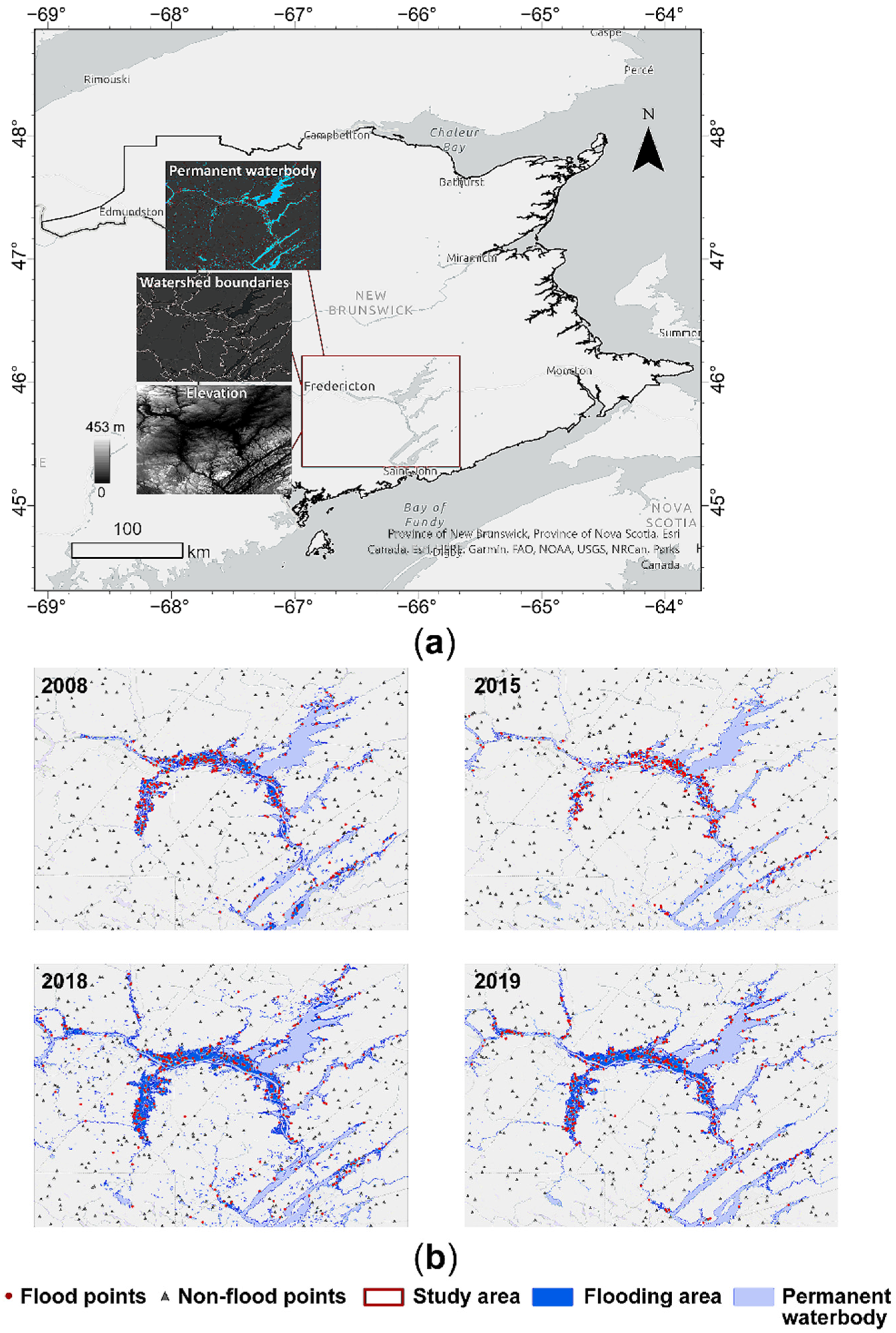
3. Study Area and Data Sources

The study area is about 10,000 km2, located in the south of the Province of New Brunswick, and covers the partial drainage basin of the St. John River (Figure 1a). The flood extent polygons of four historical large flood events that occurred in 2008, 2015, 2018, and 2019 in the area, produced from Synthetic Aperture Radar (SAR) imagery, are available at the archive of floods in Canada from the Canadian Open Government Portal [43]. Our study area covers the major flooding extent in the province in these four years. The overall extent in a certain year was created by merging the flood extent polygons on different dates in the same year. The estimated flooding area is 853.13, 708.77, 1233.38, and 1030.26 km2 in the years 2008, 2015, 2018, and 2019, respectively. A total of 600 points were randomly sampled in the study area for each of the four years, with 300 points outside the corresponding flooding extent and another 300 points within the flooding extent, while not overlapping the permanent waterbody areas (Figure 1b).
In this study, 32 explanatory factors in five categories were examined, including topographical, hydrological, geomorphic, meteorological, and anthropogenic factors. Detailed information on all influencing factors is summarized in Table 1. Except for meteorological predictors, all predictor values modeled in the DGGS were derived from open geospatial data available at the Canadian Open Government Portal (https://open.canada.ca/en/open-data (accessed on 5 May 2022)) or the provincial GeoNB Data Catalogue (http://www.snb.ca/geonb1/e/DC/catalogue-E.asp (accessed on 5 May 2022)) by applying either a quantization process or computation algorithms described in the previous literature (e.g., [15,16]). Raw geospatial data were obtained in raster or vector formats. Most of the raster data were at 30 m resolution, with the exception of the elevation data acquired from the High Resolution Digital Elevation Model [44] at 1 m resolution.
Modeled meteorological data for the 1950–2100 period in three climate change scenarios are available at the Power Analytics and Visualization for Climate Science (PAVICS) platform (https://pavics.ouranos.ca/index.html (accessed on 16 May 2022)). The gridding process of meteorological data was accomplished by the Natural Resources Canada (NRCan) using the Australian National University Spline (ANUSPLIN) implementation of the trivariate thin plate splines interpolation method and considering the effects of geospatial locations and altitudes [45]. These modeled meteorological data have been downscaled on a daily basis by applying climate model projections of temperature and precipitation using the Bias Correction/Constructed Analogues with Quantile delta mapping reordering (BCCAQv2) method, which preserves the projected changes at each quantile during quantile mapping at coarser scales [46]. The modeling process considered three climate change scenarios, reflected by three Representative Concentration Pathways (RCPs), namely RCP 2.6, RCP 4.5, and RCP 8.5, representing low, moderate, and high releases of greenhouse gases and other emissions into the atmosphere, respectively [47]. In this study, we obtained the meteorological data as summarized by standard seasons: winter (December, January, and February), spring (March, April, and May), summer (June, July, and August), and fall (September, October, and November). We investigated temperature and total precipitation in last fall (namely the fall before the spring flood in a certain year), winter, and spring, as well as days with heavy rainfall in spring (Table 1). Because the overall purpose of the meteorological simulation was to ensure that long-term statistical trends reflect historical observations, the modeled historical climate under various climate change scenarios all had similar signals [47]. For future flood forecasts, we applied meteorological values under three climate change scenarios to model predictions.
Figure 2 shows the raw meteorological data in the four historical years of the flood events (namely 2008, 2015, 2018, and 2019) and the forecasted values under three climate change scenarios for the future years of 2040, 2060, 2080, and 2100. Temperature-related variables, namely minimum, mean, or maximum daily temperature summarized by seasons, had a generally increasing trend based on the forecasts, with the scenario RCP 8.5 (i.e., high releases of greenhouse gases and other emissions) most dramatically (Figure 2). On the other hand, precipitation-related variables, such as total precipitation among different seasons and wet days over an amount threshold in spring, involved high variability and more uncertainties in their forecasts (Figure 2).
The detailed data quantization and computation processes are explained in the following sections.

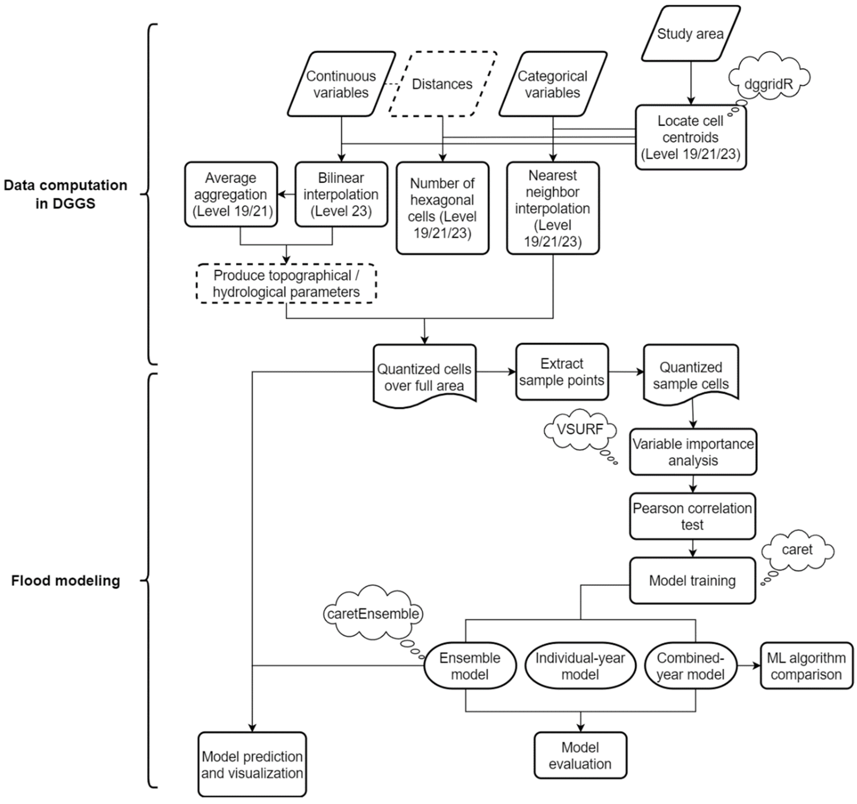
4. Data Computation in DGGS

4.1. DGGS Configuration

The ISEA3H DGGS was orientated with the latitude of the pole (λ) = 37.6895°, longitude of the pole (φ) = −51.6218°, and azimuth (α) = −72.6482°. The ISEA3H DGGS at levels 3 and 4 is visualized in Figure 3a. Following the Nyquist-Shannon sampling theorem [49], we used DGGS level 23 as the baseline in modeling processes, where the cell area was about 541.80 m2. Given that most of the raw data were at 30 m resolution, 900 m2 in area, the quantization at the finest resolution ensured no information loss from the original signals [49]. Levels 19 and 21 were also included in the modeling as two representative coarser levels, where the cell sizes were 43,885.62 and 4876.18 m2 in area, respectively, so that three modeling resolutions roughly increased at a factor of 10. The 2400 sample points described in Section 3 were quantized in the ISEA3H DGGS by converting their longitude-latitude coordinates to cell addresses of the nearest cell centroids at levels 19, 21, and 23, using the dggridR library [50]. The workflow of data computation in DGGS is shown at the top part of Figure 4, which includes the quantization of continuous variables and categorical variables, as well as the production of topographical and hydrological parameters.

4.2. Variable Quantization

A bilinear interpolation over cell centroid locations was adopted to quantize the Digital Terrain Model (DTM), including the probability of the annual minimum snow and ice, stand crown closure, total forest volume, and normalized difference vegetation index (Table 1), which were all continuous values and originally encoded in the GeoTIFF format, to the ISEA3H DGGS at level 23. The nearest four pixel centers were considered as inputs for each hexagonal centroid during the bilinear interpolation process (Figure 5a). A mean aggregation was applied to quantize the cells at coarser levels, meaning using the mean value of the seven child cells to quantize their parent cell at the immediately coarser level (Figure 3b). A nearest-neighbor interpolation (Figure 5b) was used to quantize categorical variables including the land cover classes, soil types, surficial geology types, and binary wetland classification at each modeling level of the DGGS (Table 1). All datasets, originally in vector formats, were converted through a rasterization process at 30 m resolution before quantization. By applying a binary classification on the quantized land cover classes, the impervious areas were detected and encoded in the DGGS (cells assigned the value 1 versus 0 for the non-impervious areas). The major permanent waterbodies (and road networks) were rasterized at 30 m resolution and then quantized by applying a nearest-neighbor interpolation on the ISEA3H DGGS at the three modeling resolutions (levels 19, 21, and 23). The number of hexagonal cells between the nearest waterbody (or road network) cell and the target cell was used as the distance to the nearest waterbody (or road network) in the DGGS. All cells quantized as permanent waterbodies or road networks were assigned a zero distance. All meteorological data, originally organized in the NetCDF format at 300-arcsecond spatial resolution, were quantized in the ISEA3H DGGS by applying a bilinear interpolation at the three levels (levels 19, 21, and 23) for each modeling year (years 2008, 2015, 2018, and 2019). Because of the property of discreteness, DGGS cells in the study area were divided into chunks and the quantization processes of cell chunks were conducted in a parallel manner.

4.3. Topographical and Hydrological Parameters Computation

Both the topographical parameters (aspect, slope, curvature, and roughness) and topographical indices (terrain roughness index and topographic position index) were calculated based on the quantized DTM values at each modeling level (levels 19, 21, and 23), following their definition equations [51,52] and the methodologies introduced by Li, McGrath and Stefanakis [15]. Specifically, the slope and aspect values were computed by the finite-difference algorithm (Figure 6b), where elevation differences of each central cell’s six neighbors along three axes of the hexagonal grid were projected to two orthogonal axes, and the slope and aspect of the central cell were calculated based on the combination of two orthogonal partial derivatives [15,53]. Each neighbor cell was assigned the same weight in the computation because of the uniform adjacency of cells in a hexagonal grid. Li, McGrath and Stefanakis [15] implemented and compared five algorithms to derive slope and aspect values on hexagonal grids and the finite-difference algorithm stood out because of its short computation time. The roughness was calculated within the first-ring-neighborhood, i.e., the six direct neighbors for each central cell. As suggested by Li, McGrath and Stefanakis [16], the D6 algorithm was used to produce the flow routing grid (Figure 6c), where the flow of a center cell was always routed to the neighboring cell with the lowest elevation, following the depression-filling process by the Priority-Flood algorithm [16,54,55]. Then, the flow accumulation was computed by recursively examining the inflow areas for each cell based on the flow routing grid. The hydrological indices (stream power index and topographic wetness index) were computed accordingly, with the flow accumulation and slope gradient as input parameters [16,56,57]. Except for the depression-filling process and the calculation of flow accumulation, which required us to consider the distant cells at each iteration, production of topographical and hydrological parameters was parallelized taking advantage of the discreteness of DGGS cells.

5. Flood Modeling

The flood modeling in this study involved several steps, including the variable importance analysis, correlation test, model training, model evaluation, model comparison, and model predictions and visualization, as shown at the bottom part of the workflow in Figure 4. The detailed modeling process is explained below.

5.1. Variable Importance Analysis

We included the individual-year modeling and combined-year modeling in the variable importance analysis, modeling training, and model evaluation processes. The individual-year modeling was based on 600 sample points in each historic year, and the combined-year modeling was conducted using all four years’ sample points. Because of the large group of candidate predictors, we conducted a variable importance analysis on full sample datasets using R library VSURF [58] to determine the most important predictors across the modeling years and levels. VSURF employs a two-stage strategy essentially based on the RF algorithm and returns two subsets of important variables: the first subset is used for model interpretation (hereafter referred to as “interp” variables), and the second subset, containing refined variables by avoiding redundancy, is used for model prediction (hereafter referred to as “pred” variables; [58]). We applied the VSURF algorithm to individual-year modeling and combined-year modeling at the three modeling resolutions. The “pred” variable list was considered in training both individual-year models and combined-year models. To further reduce the redundancy of predictor variables, additional Pearson correlation tests were run among each candidate predictor list for both individual-year modeling and combined-year modeling. Highly correlated variables (r > 0.7) with lower variable importance were filtered out unless they were in different variable categories according to Table 1.

5.2. Model Training, Evaluation, and Comparison

Based on 70% of sample data with finalized predictor lists, individual-year models and combined-year models were trained by RF, ANN, MLP, and SVM algorithms using the R library Caret [59] at each modeling level of the DGGS. Specifically, “rf”, “nnet”, “mlp”, and “svmRadial” were used as the “method” parameters and a bootstrap resampling was applied in the Caret’s model training procedures. The 70% training data shared the same resampling profile for each machine learning algorithm. Model training processes of these four algorithms were controlled using the same set of controlling parameters, where “classProbs = True” guarantees class probabilities should be calculated for held-out samples during the resampling, “summaryFunction = twoClassSummary” allows the sensitivity, specificity, and area under the Receiver Operating Characteristic (ROC) curve to be computed in the model results, and “allowParallel = True” governs that the modeling process uses the parallel processing. Centering and scaling were used to preprocess the training data before each modeling process. Models were tuned by a set of key parameters, and the final model was determined algorithmically with the optimized ROC value in model iterations. The initial values of key parameters and the optimization procedure applied to both individual-year models and combined-year models. The initial key parameters used in four algorithms are listed as follows.
  • RF (“rf”): “ntree” = 500, and “mtry” = square roots of number of predictor variables;
  • ANN (“nnet”): “size” = 5, and “decay” = 0;
  • MLP (“mlp”): “size” = 5;
  • SVM (“svmRadial”): “sigma” = 0.5, and “C” = 1.
Model performance metrics including the accuracy, kappa, and Area Under the ROC Curve (AUC) were calculated based on the rest 30% testing data, resulting from each of the four machine learning algorithms, for all individual-year models and combined-year models at three modeling levels. The accuracy and kappa were calculated as [60]:
a c c u r a c y = T P + T N T P + F P + T N + F N
k a p p a = ( T P + T N ) ( ( T P + F N ) ( T P + F P ) + ( F P + T N ) ( F N + T N ) ) 1 ( ( T P + F N ) ( T P + F P ) + ( F P + T N ) ( F N + T N ) )
where TP is the true positive, meaning the number of samples correctly classified as flooding sites; TN is the true negative, calculated as the number of samples correctly classified as non-flooding sites; FP is the false positive, which is the number of samples incorrectly classified as flooding sites; and FN is the false negative, computed as the number of samples incorrectly classified as non-flooding sites.
In addition, the four machine learning algorithms on combined-year models were compared to each other by summarized ROC, sensitivity, and specificity of each resampling iteration in model training processes. These metrics were comparable due to the same resampling profile during the model training. Paired t-tests were also conducted to quantitatively assess the difference among the machine learning algorithms in the unit of the average resampled area under the ROC curve.

5.3. Ensemble Model and Predictions

To compose a standard model across resolutions for flood predictions, we finalized a list of predictor variables by examining those common in the “interp” lists based on combined-year data across multiple resolutions after filtering out the highly correlated variables. An ensemble model was then built based on combined-year data, combining four machine learning algorithms by the generalized linear model method using “caretStack” strategy in the caretEnsemble library [61]. The ensemble model was trained by the combined-year data and applied to all DGGS cells in the entire study area with the meteorological data in each year of 2008, 2015, 2018, and 2019 at the three resolutions 19, 21, and 23. In addition, we replaced the meteorological data in the model with forecasted values under three climate change scenarios for the future years of 2040, 2060, 2080, and 2100 to better understand the impact of climate change on flood risks.

6. Results

6.1. Top Predictor Variables

Table 2 summarizes the top predictor variables by both “interp” and “pred” steps according to the VSURF algorithm for all individual-year models and combined-year models at all modeling levels of the DGGS. Although different sets of variables were identified in different years or resolutions due to different group of sample points used, the important predictor variables appeared repeatedly in the individual-year models and combined-year models.
In general, elevation was the most important predictor variable, followed by distances to the nearest permanent waterbodies. With all 32 variables as input to the VSURF algorithm, the mean variable importance of elevations in combined-year models was 0.283 (σ = 0.002), 0.285 (σ = 0.003), and 0.292 (σ = 0.002), and the out-of-bag errors were 0.09, 0.11, and 0.11, at levels 19, 21, and 23, respectively. The variable importance of elevations was much higher than that of the second important variable, distances to the nearest permanent waterbodies, whose mean variable importance was 0.042 (σ = 0.001), 0.053 (σ = 0.001), and 0.052 (σ = 0.001) in combined-year models at levels 19, 21, and 23, respectively.
The mean temperature in spring and the mean temperature in last fall (namely the fall before the spring flood in a certain year) were the top two meteorological variables, at least one of which was included in each individual-year model and combined-year model at all DGGS modeling levels (Table 2). In addition, the mean temperature in winter and the total precipitation in last fall were contained by “interp” models based on combined-year data at the three resolutions (Table 2). Other relatively important predictor variables were the slope, roughness, probability of the annual minimum snow and ice presence, the mean daily maximum temperature in spring, total forest volume, and surficial geology types, which were all included in the “interp” of at least one individual-year model across three resolutions (Table 2).
The Pearson correlation tests were conducted to further reduce the variable redundancy for model prediction. A high correlation (r > 0.7) was commonly observed among the terrain-derived variables of slope, curvature, roughness, and terrain roughness index, the hydrological variables flow accumulation and topographic wetness index, and a few meteorological variables such as mean temperature in spring, mean daily maximum temperature in spring, and mean temperature in last fall. The highly correlated predictor variables (r > 0.7) with lower variable importance were removed from the variable lists determined by the VSURF algorithm for both the individual-year models and combined-year models. In addition, in a few individual-year model tests, elevations and temperature-related meteorological variables (e.g., mean temperature in spring) had a negative correlation coefficient smaller than −0.7, in which cases these variables were retained in the model predictors given that they were classified in different variable categories. Table 3 summarizes the final predictor variable lists at the three DGGS modeling resolutions.

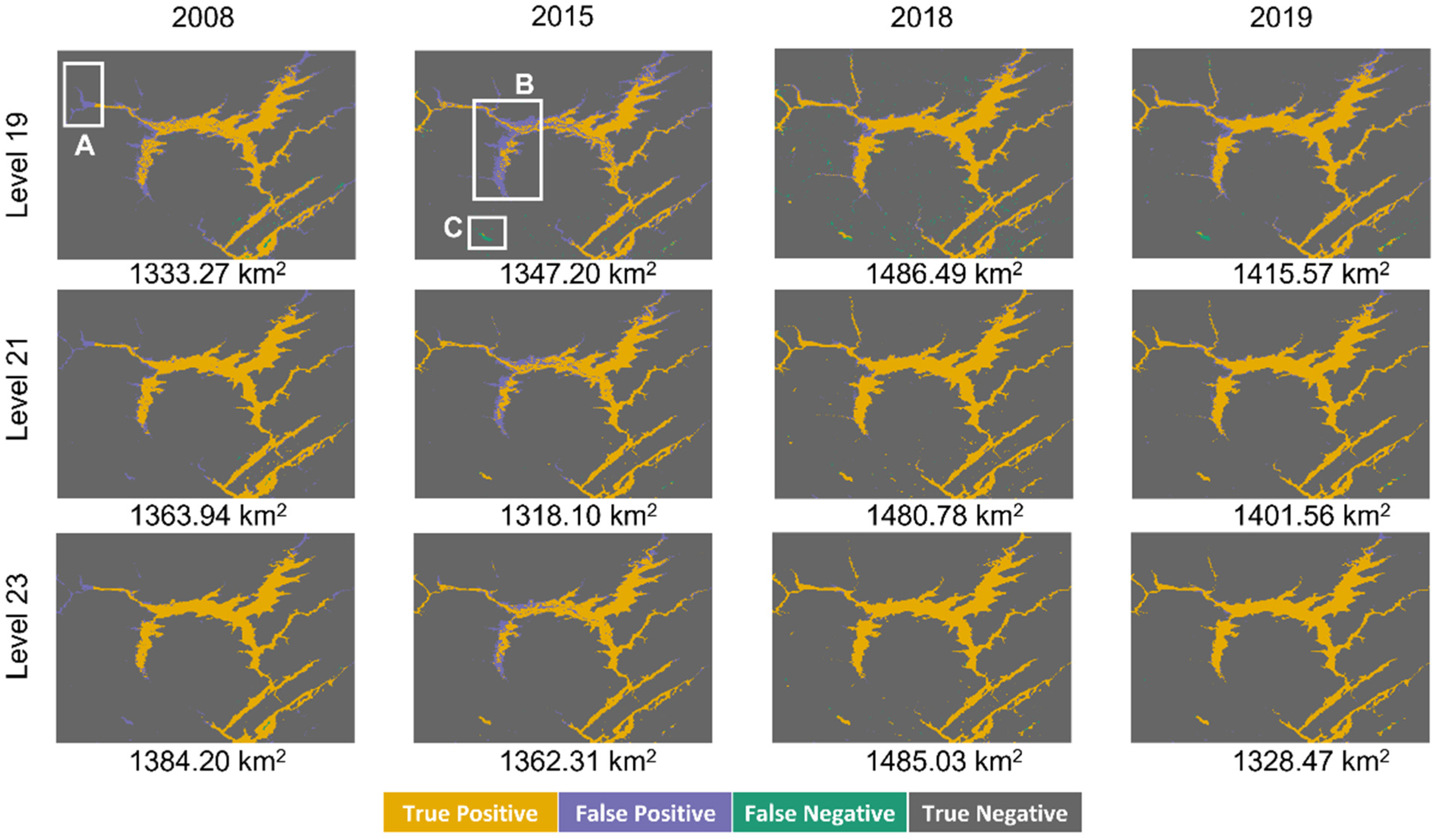
6.2. Individual-Year Models and Combined-Year Models

For both individual-year models and combined-year models, the accuracy, kappa, and AUC were computed based on the 30% testing data. According to the model performance metrics, the performance was relatively the same at all three levels, where the accuracy, kappa, and AUC of the four machine learning algorithms were greater than 0.89, 0.79, and 0.93, respectively (Figure 7). The performance of the combined-year model generally represented the average performance of the four individual-year models at a certain DGGS level (Figure 7). The individual-year model in 2018 had a slightly lower model performance, as reflected by the kappa, at the three DGGS levels (Figure 7).
Figure 8 shows the ROC, sensitivity (i.e., true positive rate), and specificity (i.e., true negative rate) of the combined-year models using the four machine learning algorithms during the iterative model training process at the three levels. Generally, the ANN had the best performance at level 19, and the RF performed the best at levels 21 and 23 (Figure 8). The ANN led to the highest ROC and sensitivity at level 19, and the RF had the highest ROC and specificity at levels 21 and 23, in terms of the mean value (Figure 8). At finer resolutions, significant differences (p < 0.05) were observed in more paired t-tests among machine learning algorithms (Figure 9). Specifically, three model pairs’ performances were significantly different (p < 0.05) in terms of ROC and specificity at level 19 while five model pairs showed significant differences at the finest level 23 (Figure 9). In terms of the calculated sensitivity, none of the models were significantly (p < 0.05) different at level 19, and two and three pairs of models had significant differences at levels 21 and 23 (Figure 9). Over the three levels, SVM led to the lowest specificity, which was significantly different (p < 0.05) from the other three machine learning algorithms (Figure 9).

6.3. Predicted Floods by Ensemble Models with Historical Meteorological Data

The predictor variables included in the ensemble model were the elevation, distances to the nearest permanent waterbodies, mean temperature in spring, roughness, surficial geology types, probability of the annual minimum snow and ice, stream power index, mean temperature in winter, total forest volume, total precipitation in last fall, normalized difference vegetation index, and topographic wetness index, ordered by their general importance. Tested by 30% of the sample data, the model performance of the ensemble model remained at a high level, with an accuracy of 0.93, 0.96, and 0.96 at levels 19, 21, and 23, respectively. The predicted flooding area in the years 2008, 2015, 2018, and 2019 was calculated by multiplying the DGGS cell size at a certain resolution and the number of cells predicted to be flooded with a probability higher than 50%. The average forecasted flooding area was 1360.47, 1342.54, 1484.10, and 1381.87 km2 across the three resolutions in the years 2008, 2015, 2018, and 2019, respectively, which was higher than the observation especially in the years 2008 and 2015.
Figure 10 demonstrates the spatial distribution of the true positive, true negative, false positive, and false negative cells by comparing the forecasted results to observations at the three levels. In 2008, the cells with false positives, meaning to be predicted as flooding cells while without a flooding observation, were mainly clustered in the northeast region (area A in Figure 10), which was likely due to the incomplete flooding observation around this area in 2008 (Figure 1b). The false positive cells in 2015 were congregated in area B (Figure 10) which was low in elevation and was not reported as a flooding area based on the historical flooding observation (Figure 1b). Area C experienced false negative predictions in years 2015, 2018, and 2019 at level 19, while such false predictions were mitigated at finer resolution levels 21 and 23 (Figure 10).

6.4. Predicted Floods by Ensemble Models with Future Meteorological Conditions

The mean temperature in spring, mean temperature in winter, and total precipitation in last fall (namely the fall before the spring flood in a certain year) were three meteorological variables included in the ensemble model, ordered by their relative importance. We predicted future flooding areas using the ensemble model by adding forecasted meteorological variables step-wisely based on their relative variable importance and compared the predicted area with observed flooding in 2019, 1030.26 km2 in area as the baseline, because it was the most recent major flood event in the study area.
With the mean temperature in spring as the only meteorological predictor changing over time in the model, the predicted flooding area increased with higher RCPs over the years at three resolutions (Figure 11a). It was noted that the mean temperature in spring was forecasted to be higher in higher-concentration climate change scenarios (Figure 2), revealing its positive influence on flood risks. The predicted flooding area in the optimistic climate change scenario, namely RCP 2.6, was the lowest in 2060 and highest in 2100 at all three resolutions (Figure 11a), in line with the changing trend of mean temperature in spring in RCP 2.6 over the years (Figure 2). A greater difference in predicted flooding areas among climate change scenarios was shown at finer resolutions (Figure 11a). For example, the predicted flooding area in 2060 ranged from 1856.32 to 2831.98 km2 (180–275% of 2019 flooding area), 1649.51 to 3143.09 km2 (160–305% of 2019 flooding area), 1589.30 to 3351.62 km2 (154–325% of 2019 flooding area) among three climate change scenarios at levels 19, 21, and 23, respectively (Figure 11a).
When adding the second and third meteorological variables, namely mean temperature in winter and total precipitation in last fall in model prediction, the predicted flooding area generally decreased at all three modeling levels (Figure 11). The highest flooding area prediction over the climate change scenarios across the years was 2895.03, 3173.20, and 3348.34 km2 with the first meteorological variable in model prediction (Figure 11a); 2338.69, 2132.64, and 2070.82 km2 with the first two meteorological variables in model prediction (Figure 11b); and 2091.43, 1648.42, and 1576.30 km2 with all three meteorological variables in model prediction (Figure 11c), at levels 19, 21, and 23, respectively.
Moreover, when step-wisely adding the meteorological variables to the prediction model, the differences among the scenarios were gradually reduced with regard to the predicted flooding area, especially at level 23 (Figure 11). At level 23, the range (differences between the minimum and maximum) of predicted flooding areas in multiple climate change scenarios was 669.67, 1761.74, 947.84, and 525.43 km2 when the mean temperature in spring was included as the only changing variable in the model over time, and 82.42, 20.61, 175.14, and 113.33 km2 when all three meteorological variables were included in the model, in 2040, 2060, 2080, and 2100, respectively (Figure 11). Figure 12 visualizes the predicted flooding extent and probabilities of flooding results from the ensemble model for all three meteorological variables (i.e., Figure 11c) under three climate change scenarios around Fredericton, New Brunswick, in 2040, 2060, 2080, and 2100 at level 23.

7. Discussion

7.1. Influencing Factors and Forecasts of Flood Risks

Elevation and proximity to permanent waterbodies were identified as the most important influencing factors on flood risks, by investigating not only individual years’ data but also combined years’ data. Locations with lower elevations and closer to permanent waterbodies tend to be vulnerable to flood risks, as visualized in the flooding maps (Figure 12). The topographical parameters describing the complexity of terrain surfaces, such as the roughness, slope, and terrain roughness index, showed relatively high importance in the model interpretation compared to the other non-climate variables. These determined top influencing factors were in agreement with other research on inland floods using machine learning methods (e.g., [17,18,19]).
In terms of the climate conditions, the highly correlated factors of mean temperature in spring and mean temperature in last fall were essential factors in flood risks. Based on all four years’ sampling data, the variable importance of the mean temperature in spring was higher than that of the mean temperature in last fall and thus included in the ensemble model for flood predictions. According to the forecasted climate conditions under three emission scenarios, the mean temperature in spring tends to increase in higher-concentration emission scenarios. We noticed that the predicted flooding extent was larger in higher RCP scenarios when including the mean temperature in spring as the only changing meteorological variable in the model, which reflected the positive effect of mean temperature in spring on flood risks. As reported by the Government of New Brunswick, snow melt and ice jams are significant causes of New Brunswick floods in spring, where increasing temperature and heavy rainfall are the main triggers for flood events [20]. We also found that with the forecasted mean temperature in winter and total precipitation of the last fall added to the prediction model, the projected flood risks were mitigated over time. The flooding extent can be 135% to 203% of the 2019 flood area including three meteorological factors in the model by the year 2100. Nevertheless, it should be noted the purpose was not to provide a specific flooding susceptibility prediction in the future 80 years, which cannot be validated at the present, but to understand the possible impact of climate change on flood risks by predicting future flooding extent. Three climate change scenarios contained different hypotheses of how nature or society will behave in terms of greenhouse gas emissions.
The model performance remained at high levels, as suggested by performance metrics calculated based on 30% testing data for both individual-year models and combined-year models. Nonetheless, flooding extent can be overestimated by applying the ensemble model to historical flood estimates, especially in the years 2008 and 2015 when relatively less flooding area was derived and digitalized from SAR imagery. The quality of flood extent products, used as observation data in this paper, was affected by a few factors such as sensor parameters and environmental conditions at the time of image acquisition, which can impose limitations on model predictions [62].

7.2. Effects of Modeling Resolutions

We conducted the flood modeling at levels 19, 21, and 23 in the ISEA3H DGGS where the cell size was approximately reduced by a factor of 9 between levels 19 and 21, and levels 21 and 23. Top explanatory variables generally agreed among the three levels, especially when combining the four years of data in one model. The model performance was overall consistent across the three levels based on testing data. Based on training data, four tested machine learning algorithms showed more differences at finer resolutions in terms of model performance metrics. By applying forecasted climate conditions to the ensemble model under three emission scenarios in the future, it was found that the differences in predicted flooding areas were most vulnerable to various emission scenarios at the finest modeling resolution. More specifically, predictions with forecasted mean temperature in spring showed the greatest difference among climate change scenarios in terms of flooding area at level 23. On the other hand, having mean temperature in spring, mean temperature in winter, and total precipitation in last fall in the ensemble model led to the least difference in projected flooding area among climate change scenarios at the finest resolution.

7.3. Flood Modeling in Hexagonal DGGS

In this research, we utilized the ISEA3H DGGS as a standardized, scalable data fabric and applied data mining algorithms in external libraries to solve a real-world problem, flood mapping. Although this was not the first attempt to model flood inundation by using general DGGS, this study managed to standardize multi-source geospatial data, derive parameters via analytical operations, and retrieve data at multiple resolutions in a pure hexagonal DGGS environment, which was not accomplished in the past. Specifically, we computed topographical and hydrological parameters such as the slope, aspect, roughness, curvature, flow direction, and flow accumulation, as well as topographical or hydrological indices including terrain roughness index, topographic position index, stream power index, and topographic wetness index directly in the DGGS environment based on the hexagonal geometries at multiple scales. Additionally, distances to nearby permanent waterbodies and roads were represented by the number of hexagonal cells at a certain resolution. One or more explanatory variables mentioned above were involved in the individual-year models, combined-year models, and ensemble models in this paper. Previously, a height above the nearest drainage flood risk modeling system was developed based on a hexagonal DGGS, while a few input parameters like drainage accumulation and watershed boundaries were produced upon rectangular grid meshes, and the data values were then converted to the DGGS platform [10]. The quantization and production of explanatory factor values directly in a DGGS can improve the consistency of the modeling process and reduce uncertainty propagation. Because of the discrete property of DGGS cells, the quantization process and most of the analytical operations in DGGS can be appropriately conducted in a parallel fashion, which can lower the wall-clock time of data computation.
We demonstrated the application of several machine learning algorithms to DGGS-driven datasets in the flood mapping domain. The linkage to external machine learning libraries, as shown in this paper, was feasible given that the data mining algorithms were based on a training dataset that consisted of individual DGGS cells at a certain resolution. The aperture of 3 was particularly employed in the hexagonal DGGS, and the methodology proposed in this paper can be adjusted to other hexagonal DGGS with a higher aperture, such as 4 or 7, where the effects of modeling resolution can be more apparent. On the other hand, the incorporation of DGGS and bottom-up predictive models such as cellular automata and agent-based modeling requires further development because the neighborhood relationship over the grid cells is an essential component of the modeling process. Although not using a hierarchical grid system, Douass and Kbir [14] gave an example of calculating water flow dynamics and delineating flood zones with the cellular automata-based algorithm in hexagonal grid meshes. Conducting these bottom-up predictive models in a hexagonal DGGS environment can be promising if the neighborhood navigation is supported by a cell indexing mechanism, which is exemplified by the Quadrilateral 2-Dimensional Integer (Q2DI) indexing implemented in the DGGRID library [63]. Regarding the modeling at multi-resolutions, the concept of neighborhood navigation needs to be extended across resolutions, or such hierarchical operators can be generalized in a topology-independent manner, as noted by Kiester and Sahr [64].

8. Conclusions

This work focused on multi-scale flood mapping in southern New Brunswick by four separate machine learning algorithms including the RF, ANN, MLP, and SVM, and the ensemble model combing these four algorithms based on both four individual-years’ observation data and combined-years’ data. A total of 32 explanatory factors in five categories were involved in the initial variable importance analysis, and subsets of them were included in the following modeling process at multiple resolutions according to their relative importance and correlations. We also estimated the future flooding extent under three climate change scenarios by replacing the historical climate conditions with their forecasted values in trained ensemble models. The ISEA3H DGGS was adopted as the base standardized data fabric for predictor variable quantization and computation, which benefited the integration process of multi-source geospatial data and provided the hierarchical framework for multi-scale analysis. Furthermore, producing explanatory factor values, such as roughness and flow accumulation, directly in a DGGS can improve the consistency of modeling processes and help to avoid further uncertainty propagation. Our results showed that elevations and proximity to permanent waterbodies were key factors affecting flood risks in the study area, suggested by both individual-year models and combined-year models with high model performance. The rising mean temperature in spring can lead to higher flood risk, considering that snow melt is one of the primary trigger factors of floods around our study area. Differences in model performance among four tested machine learning algorithms became more obvious at finer modeling resolutions. The results of this study helped to identify the top influencing factors and understand the impact of climate change on flood risks, which was meaningful in future flood warnings. Our research also demonstrated the feasibility of incorporating external machine-learning libraries with a DGGS-based data framework. Future studies can explore the advanced algorithms in flood modeling, such as MAXENT, XGBoost, and MARS, and more development is needed for the incorporation of bottom-up predictive models involving topological relationships. The methodology proposed in this research can also be adjusted to fit different DGGS configurations and the comparison of the modeling results between various DGGS can be examined in the future.
Mingke Li 1,*, Heather McGrath 2 and Emmanuel Stefanakis

Author Contributions

Conceptualization, Emmanuel Stefanakis, Heather McGrath and Mingke Li; methodology, Heather McGrath and Mingke Li; software, Mingke Li; validation, Heather McGrath and Mingke Li; formal analysis, Mingke Li; investigation, Mingke Li; resources, Emmanuel Stefanakis and Heather McGrath; writing—original draft preparation, Mingke Li; writing—review and editing, Emmanuel Stefanakis and Heather McGrath; visualization, Mingke Li; supervision, Emmanuel Stefanakis and Heather McGrath. All authors have read and agreed to the published version of the manuscript.

Funding

This research was funded by Natural Resources Canada (NRCan) with NRCan contribution number/Numéro de contribution de RNCan: 20220363. We acknowledge the extra funding from the De l’observation de la terre aux services d’information déci-sionnelle (CREATE DOTS) program.

Institutional Review Board Statement

Not applicable.

Informed Consent Statement

Not applicable.

Data Availability Statement

Acknowledgments

We thank the PAVICS platform (Ouranos and Computer Research Institute of Montreal, 2018–2022) for meteorological data access. PAVICS is funded through Ouranos, Computer Research Institute of Montreal, Environment and Climate Change Canada (ECCC), CANARIE, the Fonds Vert and the Fonds d’électrification et de changements climatiques, the Canadian Foundation for Innovation (CFI), and the Fonds de Recherche du Québec (FRQ).

Conflicts of Interest

The authors declare no conflict of interest.

Abbreviations

AcronymsDescription
ANNArtificial Neural Networks
ANUSPLINAustralian National University Spline
BCCAQv2Bias Correction/Constructed Analogues with Quantile delta mapping reordering
DGGSDiscrete Global Grid Systems
DTMDigital Terrain Model
GISGeographic Information Systems
ISEA3HIcosahedral Snyder Equal Area Aperture 3 Hexagonal Grid
LiDARLight Detection and Ranging
MARSMultivariate Adaptive Regression Splines
MAXENTMaximum Entropy
MLPMultilayer Perceptron
NRCanNatural Resources Canada
PAVICSPower Analytics and Visualization for Climate Science
Q2DIQuadrilateral 2-Dimensional Integer
RCPRepresentative Concentration Pathway
RFRandom Forest
ROCReceiver Operating Characteristic
SARSynthetic Aperture Radar
SVMSupport Vector Machine
XGBoostExtreme Gradient Boosting

References

  1. Goodchild, M.F. Reimagining the history of GIS. Ann. GIS 2018, 24, 1–8. [Google Scholar] [CrossRef]
  2. Dutton, G. Modelling locational uncertainty via hierarchical tessellation. In Accuracy of Spatial Databases; Goodchild, M.F., Gopal, S., Eds.; Taylor & Francis: Abingdon, UK, 1989; pp. 81–91. [Google Scholar]
  3. Alderson, T.; Purss, M.; Du, X.; Mahdavi-Amiri, A.; Samavati, F. Digital earth platforms. In Manual of Digital Earth; Guo, H., Goodchild, M., Annoni, A., Eds.; Springer: Singapore, 2020; pp. 25–54. [Google Scholar]
  4. OGC. Topic 21: Discrete Global Grid System Abstract Specification. Available online: http://www.opengis.net/doc/AS/dggs/1.0 (accessed on 15 November 2019).
  5. Robertson, C.; Chaudhuri, C.; Hojati, M.; Roberts, S.A. An integrated environmental analytics system (IDEAS) based on a DGGS. ISPRS J. Photogramm. Remote Sens. 2020, 162, 214–228. [Google Scholar] [CrossRef]
  6. Rawson, A.; Sabeur, Z.; Brito, M. Intelligent geospatial maritime risk analytics using the Discrete Global Grid System. Big Earth Data 2022, 6, 294–322. [Google Scholar] [CrossRef]
  7. Bousquin, J. Discrete Global Grid Systems as scalable geospatial frameworks for characterizing coastal environments. Environ. Model. Softw. 2021, 146, 105210. [Google Scholar] [CrossRef] [PubMed]
  8. Li, M.; McGrath, H.; Stefanakis, E. Integration of heterogeneous terrain data into Discrete Global Grid Systems. Cartogr. Geogr. Inf. Sci. 2021, 48, 546–564. [Google Scholar] [CrossRef]
  9. Chen, A.S.; Evans, B.; Djordjević, S.; Savić, D.A. A coarse-grid approach to representing building blockage effects in 2D urban flood modelling. J. Hydrol. 2012, 426–427, 1–16. [Google Scholar] [CrossRef] [Green Version]
  10. Chaudhuri, C.; Gray, A.; Robertson, C. InundatEd-v1.0: A height above nearest drainage (HAND)-based flood risk modeling system using a discrete global grid system. Geosci. Model Dev. 2021, 14, 3295–3315. [Google Scholar] [CrossRef]
  11. Wang, L.; Ai, T.; Shen, Y.; Li, J. The isotropic organization of DEM structure and extraction of valley lines using hexagonal grid. Trans. GIS 2020, 24, 483–507. [Google Scholar] [CrossRef]
  12. Liao, C.; Tesfa, T.; Duan, Z.; Leung, L.R. Watershed delineation on a hexagonal mesh grid. Environ. Model. Softw. 2020, 128, 104702. [Google Scholar] [CrossRef]
  13. Liao, C.; Zhou, T.; Xu, D.; Barnes, R.; Bisht, G.; Li, H.-Y.; Tan, Z.; Tesfa, T.; Duan, Z.; Engwirda, D.; et al. Advances in hexagon mesh-based flow direction modeling. Adv. Water Resour. 2022, 160, 104099. [Google Scholar] [CrossRef]
  14. Douass, S.; Kbir, M.A. Flood zones detection using a runoff model built on hexagonal shape based cellular automata. Int. J. Eng. Trends Technol. 2020, 68, 68–74. [Google Scholar] [CrossRef]
  15. Li, M.; McGrath, H.; Stefanakis, E. Multi-resolution topographic analysis in hexagonal Discrete Global Grid Systems. Int. J. Appl. Earth Obs. Geoinf. 2022, 113, 102985. [Google Scholar] [CrossRef]
  16. Li, M.; McGrath, H.; Stefanakis, E. Geovisualization of hydrological flow in hexagonal grid systems. Geographies 2022, 2, 227–244. [Google Scholar] [CrossRef]
  17. Tehrany, M.S.; Jones, S.; Shabani, F. Identifying the essential flood conditioning factors for flood prone area mapping using machine learning techniques. Catena 2019, 175, 174–192. [Google Scholar] [CrossRef]
  18. Zhao, G.; Pang, B.; Xu, Z.; Peng, D.; Xu, L. Assessment of urban flood susceptibility using semi-supervised machine learning model. Sci. Total Environ. 2019, 659, 940–949. [Google Scholar] [CrossRef]
  19. McGrath, H.; Gohl, P.N. Accessing the impact of meteorological variables on machine learning flood susceptibility mapping. Remote Sens. 2022, 14, 1656. [Google Scholar] [CrossRef]
  20. GNB. New Brunswick’s Flood Risk Reduction Strategy. Available online: https://www2.gnb.ca/content/dam/gnb/Departments/env/pdf/Flooding-Inondations/NBFloodRiskReductionStrategy.pdf (accessed on 14 September 2022).
  21. Mosavi, A.; Ozturk, P.; Chau, K.-W. Flood prediction using machine learning models: Literature review. Water 2018, 10, 1536. [Google Scholar] [CrossRef] [Green Version]
  22. Abdullah, M.F.; Siraj, S.; Hodgett, R.E. An overview of multi-criteria decision analysis (MCDA) application in managing water-related disaster events: Analyzing 20 years of literature for food and drought events. Water 2021, 13, 1358. [Google Scholar] [CrossRef]
  23. Lin, L.; Di, L.; Yu, E.G.; Kang, L.; Shrestha, R.; Rahman, M.S.; Tang, J.; Deng, M.; Sun, Z.; Zhang, C.; et al. A review of remote sensing in flood assessment. In Proceedings of the 2016 Fifth International Conference on Agro-Geoinformatics (Agro-Geoinformatics), Tianjin, China, 2016, 18–20 July 2016; p. 4. [Google Scholar]
  24. Tehrany, M.S.; Pradhan, B.; Jebur, M.N. Flood susceptibility mapping using a novel ensemble weights-of-evidence and support vector machine models in GIS. J. Hydrol. 2014, 512, 332–343. [Google Scholar] [CrossRef]
  25. Lohani, A.K.; Kumar, R.; Singh, R.D. Hydrological time series modeling: A comparison between adaptive neuro-fuzzy, neural network and autoregressive techniques. J. Hydrol. 2012, 442–443, 23–35. [Google Scholar] [CrossRef]
  26. Kim, S.; Singh, V.P. Flood forecasting using neural computing techniques and conceptual class segregation. JAWRA J. Am. Water Resour. Assoc. 2013, 49, 1421–1435. [Google Scholar] [CrossRef]
  27. Lin, J.; He, P.; Yang, L.; He, X.; Lu, S.; Liu, D. Predicting future urban waterlogging-prone areas by coupling the maximum entropy and FLUS model. Sustain. Cities Soc. 2022, 80, 103812. [Google Scholar] [CrossRef]
  28. Siahkamari, S.; Haghizadeh, A.; Zeinivand, H.; Tahmasebipour, N.; Rahmati, O. Spatial prediction of flood-susceptible areas using frequency ratio and maximum entropy models. Geocarto Int. 2018, 33, 927–941. [Google Scholar] [CrossRef]
  29. Abedi, R.; Costache, R.; Shafizadeh-Moghadam, H.; Pham, Q.B. Flash-flood susceptibility mapping based on XGBoost, random forest and boosted regression trees. Geocarto Int. 2022, 37, 5479–5496. [Google Scholar] [CrossRef]
  30. Bui, D.T.; Hoang, N.D.; Pham, T.D.; Ngo, P.T.T.; Hoa, P.V.; Minh, N.Q.; Tran, X.T.; Samui, P. A new intelligence approach based on GIS-based Multivariate Adaptive Regression Splines and metaheuristic optimization for predicting flash flood susceptible areas at high-frequency tropical typhoon area. J. Hydrology 2019, 575, 314–326. [Google Scholar] [CrossRef]
  31. Berger, A.; Della Pietra, S.A.; Della Pietra, V.J. A maximum entropy approach to natural language processing. Comput. Linguist. 1996, 22, 39–71. [Google Scholar]
  32. Ho, T.K. Random decision forests. In Proceedings of the 3rd International Conference on Document Analysis and Recognition 1995, Montreal, QC, Canada, 14–16 August 1995; pp. 278–282. [Google Scholar]
  33. Bui, D.T.; Tuan, T.A.; Klempe, H.; Pradhan, B.; Revhaug, I. Spatial prediction models for shallow landslide hazards: A comparative assessment of the efficacy of support vector machines, artificial neural networks, kernel logistic regression, and logistic model tree. Landslides 2016, 13, 361–378. [Google Scholar] [CrossRef]
  34. Wang, Z.; Lai, C.; Chen, X.; Yang, B.; Zhao, S.; Bai, X. Flood hazard risk assessment model based on random forest. J. Hydrol. 2015, 527, 1130–1141. [Google Scholar] [CrossRef]
  35. Jain, A.; Prasad Indurthy, S. Closure to “comparative analysis of event-based rainfall-runoff modeling techniques—Deterministic, statistical, and artificial neural networks” by ASHU JAIN and SKV prasad indurthy. J. Hydrol. Eng. 2004, 9, 551–553. [Google Scholar] [CrossRef]
  36. Kar, A.K.; Lohani, A.K.; Goel, N.K.; Roy, G.P.J. Development of flood forecasting system using statistical and ANN techniques in the downstream catchment of mahanadi basin, india. J. Water Resour. Prot. 2010, 2, 880. [Google Scholar]
  37. Taormina, R.; Chau, K.W.; Sethi, R. Artificial neural network simulation of hourly groundwater levels in a coastal aquifer system of the Venice lagoon. Eng. Appl. Artif. Intell. 2012, 25, 1670–1676. [Google Scholar] [CrossRef] [Green Version]
  38. Rumelhart, D.E.; Hinton, G.E.; Williams, R.J. Learning representations by back-propagating errors. Nature 1986, 323, 533–536. [Google Scholar] [CrossRef]
  39. Riad, S.; Mania, J.; Bouchaou, L.; Najjar, Y. Rainfall-runoff model usingan artificial neural network approach. Math. Comput. Model. 2004, 40, 839–846. [Google Scholar] [CrossRef]
  40. Senthil Kumar, A.R.; Sudheer, K.P.; Jain, S.K.; Agarwal, P.K. Rainfall-runoff modelling using artificial neural networks: Comparison of network types. Hydrol. Process. 2005, 19, 1277–1291. [Google Scholar] [CrossRef]
  41. Vapnik, V.; Mukherjee, S. Support vector method for multivariate density estimation. Adv. Neural Inf. Process. Syst. 2000, 4, 659–665. [Google Scholar]
  42. Dibike, Y.B.; Velickov, S.; Solomatine, D.; Abbott, M.B. Model induction with support vector machines: Introduction and applications. J. Comput. Civ. Eng. 2001, 15, 208–216. [Google Scholar] [CrossRef]
  43. NRCan. Floods in Canada—Archive. Available online: https://open.canada.ca/data/en/dataset/74144824-206e-4cea-9fb9-72925a128189 (accessed on 5 March 2022).
  44. NRCan. High Resolution Digital Elevation Model Mosaic (HRDEM Mosaic)—CanElevation Series. Available online: https://open.canada.ca/data/en/dataset/0fe65119-e96e-4a57-8bfe-9d9245fba06b (accessed on 4 March 2022).
  45. Hutchinson, M.F.; McKenney, D.W.; Lawrence, K.; Pedlar, J.H.; Hopkinson, R.F.; Milewska, E.; Papadopol, P. Development and testing of Canada-wide interpolated spatial models of daily minimum–maximum temperature and precipitation for 1961–2003. J. Appl. Meteorol. Climatol. 2009, 48, 725–741. [Google Scholar] [CrossRef]
  46. Cannon, A.J.; Sobie, S.R.; Murdock, T.Q. Bias correction of GCM precipitation by quantile mapping: How well do methods preserve changes in quantiles and extremes? J. Clim. 2015, 28, 6938–6959. [Google Scholar] [CrossRef]
  47. Bush, E.; Lemmen, D.S. Canada’s Changing Climate Report; Government of Canada: Ottawa, ON, Canada, 2019; p. 444. [Google Scholar]
  48. NRCan. New Brunswick Hydrographic Network (NBHN). Available online: https://open.canada.ca/data/en/dataset/56345831-3fdd-0e11-8a7a-3b009876bf86 (accessed on 4 March 2022).
  49. Shannon, C.E. Communication in the presence of noise. In Proceedings of the IRE; Institute of Radio Engineers: New York, NY, USA, 1949; pp. 10–21. [Google Scholar]
  50. Barnes, R.; Sahr, K. dggridR: Discrete Global Grids for R. R Package Version 2.0.4. Available online: https://github.com/r-barnes/dggridR (accessed on 5 March 2020).
  51. Guisan, A.; Weiss, S.B.; Weiss, A.D. GLM versus CCA spatial modeling of plant species distribution. Plant Ecol. 1999, 143, 107–122. [Google Scholar] [CrossRef]
  52. Riley, S.J.; DeGloria, S.D.; Elliot, R. Index that quantifies topographic heterogeneity intermountain. J. Sci. 1999, 5, 23–27. [Google Scholar]
  53. Hodgson, M.E. Comparison of angles from surface slope/aspect algorithms. Cartogr. Geogr. Inf. Syst. 1998, 25, 173–185. [Google Scholar] [CrossRef]
  54. Barnes, R. Parallel Priority-Flood depression filling for trillion cell digital elevation models on desktops or clusters. Comput. Geosci. 2016, 96, 56–68. [Google Scholar] [CrossRef] [Green Version]
  55. Barnes, R.; Lehman, C.; Mulla, D. Priority-flood: An optimal depression-filling and watershed-labeling algorithm for digital elevation models. Comput. Geosci. 2014, 62, 117–127. [Google Scholar] [CrossRef] [Green Version]
  56. Moore, I.D.; Grayson, R.B.; Ladson, A.R. Digital terrain modelling: A review of hydrological, geomorphological, and biological applications. Hydrol. Process. 1991, 5, 3–30. [Google Scholar] [CrossRef]
  57. Beven, K.J.; Kirkby, M.J. A physically based, variable contributing area model of basin hydrology / Un modèle à base physique de zone d’appel variable de l’hydrologie du bassin versant. Hydrol. Sci. Bull. 1979, 24, 43–69. [Google Scholar] [CrossRef] [Green Version]
  58. Genuer, R.; Poggi, J.M.; Tuleau-Malot, C. VSURF: An R package for variable selection using random forests. R J. 2015, 7, 19–33. [Google Scholar] [CrossRef] [Green Version]
  59. Kuhn, M. Building predictive models in R using the caret package. J. Stat. Softw. 2008, 28, 1–26. [Google Scholar] [CrossRef] [Green Version]
  60. McHugh, M.L. Interrater reliability: The kappa statistic. Biochem. Med. 2012, 22, 276–282. [Google Scholar] [CrossRef]
  61. Deane-Mayer, Z.A.; Knowles, J.E. Ensembles of Caret Models. Available online: https://github.com/zachmayer/caretEnsemble (accessed on 6 May 2022).
  62. NRCan. Floods in Canada/International Floods Product Specifications. Available online: https://open.canada.ca/data/en/dataset/74144824-206e-4cea-9fb9-72925a128189/resource/3d2e0b75-1546-4617-8bbb-ec65321b6c28 (accessed on 12 September 2022).
  63. Sahr, K. Location coding on icosahedral aperture 3 hexagon discrete global grids. Comput. Environ. Urban Syst. 2008, 32, 174–187. [Google Scholar] [CrossRef]
  64. Kiester, A.R.; Sahr, K. Planar and spherical hierarchical, multi-resolution cellular automata. Comput. Environ. Urban Syst. 2008, 32, 204–213. [Google Scholar] [CrossRef]
Figure 1. (a) Study area in southern New Brunswick, Canada; and (b) flooding extent produced from Synthetic Aperture Radar imagery in years 2008, 2015, 2018, and 2019. Digital Elevation Model data, watershed and waterbody data, and historical flood data were retrieved from Canadian Open Government Portal [43,44,48].
Ijgi 11 00627 g001
Figure 2. Meteorological data used for the past years of 2008, 2015, 2018, and 2019 and forecasted values under three climate change scenarios for the future years of 2040, 2060, 2080, and 2100. Raw data were retrieved from the Power Analytics and Visualization for Climate Science (PAVICS) platform (https://pavics.ouranos.ca/index.html (accessed on 16 May 2022)). Variable abbreviations refer to Table 1.
Ijgi 11 00627 g002
Figure 3. Illustration of (a) ISEA3H DGGS at level 3 and level 4; and (b) relationship between a parent hexagonal cell and its child cells.
Ijgi 11 00627 g003
Figure 4. Workflow of data computation and flood modeling in DGGS.
Ijgi 11 00627 g004
Figure 5. Quantization of geospatial data in the ISEA3H DGGS using (a) a bilinear interpolation; and (b) a nearest-neighbor interpolation.
Ijgi 11 00627 g005
Figure 6. Example of analytical operations in the ISEA3H DGGS: (a) center cell and its six neighbors with quantized elevation values; (b) calculating slope and aspect using the finite-difference algorithm; and (c) computing flow direction using the D6 algorithm.
Ijgi 11 00627 g006
Figure 7. Accuracy, kappa, and AUC of individual-year models and combined-year models using four machine learning algorithms, Artificial Neural Networks (ANN), Multilayer Perceptron (MLP), Random Forests (RF), and Support Vector Machine (SVM) at the three modeling levels.
Ijgi 11 00627 g007
Figure 8. ROC, sensitivity, and specificity of combined-year models using four machine learning algorithms, Artificial Neural Networks (ANN), Multilayer Perceptron (MLP), Random Forests (RF), and Support Vector Machine (SVM) during iterative model training process at the three modeling levels.
Ijgi 11 00627 g008
Figure 9. Paired t-tests in terms of ROC, sensitivity, and specificity among four machine learning algorithms, Artificial Neural Networks (ANN), Multilayer Perceptron (MLP), Random Forests (RF), and Support Vector Machine (SVM) during iterative model training process at the three modeling levels, where significant differences (p < 0.05) are highlighted with red rectangles.
Ijgi 11 00627 g009
Figure 10. Spatial distribution of true positive, true negative, false positive, and false negative cells by comparing the forecasted results from ensemble models to observations in each of the four years at the three resolution levels. Areas highlighted by red rectangles and letters A, B, and C are major false positive or false negative locations and are discussed in supporting text.
Ijgi 11 00627 g010
Figure 11. Predicted flooding area by ensemble models under three climate change scenarios with forecasted (a) mean temperature in spring; (b) mean temperature in spring and mean temperature in winter; and (c) mean temperature in spring, mean temperature in winter, and total precipitation in last fall, in the future years of 2040, 2060, 2080, and 2100 at the three levels. Bars are labeled by the ratio between the predicted flooding area and the observed flooding area in 2019 (1030.26 km2) which is marked with horizontal, dashed lines in the plots.
Ijgi 11 00627 g011
Figure 12. Visualization of (a) flooding extent; and (b) probabilities of flooding predicted by the ensemble model under three climate change scenarios around Fredericton, New Brunswick, in the years 2040, 2060, 2080, and 2100 at level 23.
Ijgi 11 00627 g012
Table 1. Summary of five categories of predictor variables and data sources.
CategoryAbbreviationDescriptionRaw Format
Terrain-deriveddtm 1Digital Terrain Model (i.e., elevations)GeoTIFF
aspAspect
slpSlope
curvCurvature
rghRoughness
triTerrain roughness index
tpiTopographic position index
HydrologicalfldirFlow direction
flaccFlow accumulation
msi 2Probability of the annual minimum snow and iceGeoTIFF
nhn 3Distance to the nearest permanent waterbodiesGeodatabase
wl 4WetlandShapefile
spiStream power index
twiTopographic wetness index
Geomorphiclc 5Land cover classesGeoTIFF
scc 6Stand crown closureGeoTIFF
tfv 7Total forest volumeGeoTIFF
ndvi 8Normalized difference vegetation indexGeoTIFF
sol 9Soil typesGeodatabase
geo 10Surficial geology typesGeodatabase
Meteorological 11fprcptotTotal precipitation in last fallNetCDF
ftgmeanMean temperature in last fall
ftnmeanMean of daily min temperature in last fall
wprcptotTotal precipitation in winter
wtgmeanMean temperature in winter
sprcptotTotal precipitation in spring
stgmeanMean temperature in spring
stxmeanMean of daily max temperature in spring
sr10Spring wet-days > 10 mm
sr20Spring wet-days > 20 mm
AnthropogeniciaImpervious areas
nrn 12Distance to the nearest major roadsShapefile
Table 2. Selected variables by VSURF library for individual-year models and combined-year models at the three DGGS modeling levels.
LevelModel YearStepSelected Variables 1
Level 19Year 2008interp 2dtm, ftgmean, stgmean, nhn, rgh, twi
pred 3dtm, ftgmean, stgmean, nhn, rgh, twi
Year 2015interpdtm, ftgmean, nhn, stgmean, tri
preddtm, ftgmean, nhn
Year 2018interpdtm, nhn, twi, stgmean, flacc, lc
preddtm, nhn, twi, stgmean
Year 2019interpdtm, nhn, twi, slp, msi, geo, tri, stgmean, rgh, stxmean, tfv, flacc, curv, ndvi
preddtm, nhn, twi, msi, geo, stgmean
Combined-yearinterpdtm, nhn, twi, rgh, tri, slp, stgmean, msi, geo, stxmean, flacc, lc, tpi, wtgmean, curv, spi, tfv, ndvi, fprcptot
preddtm, nhn, twi, stgmean, rgh
Level 21Year 2008interpdtm, ftgmean, nhn, stgmean, rgh
preddtm, ftgmean, nhn, stgmean, rgh
Year 2015interpdtm, ftgmean, nhn, rgh, slp, stgmean, tri, ftnmean, tfv, lc, ndvi, msi, wtgmean, stxmean, scc
preddtm, ftgmean, nhn, stgmean, tfv
Year 2018interpdtm, nhn, stgmean
preddtm, nhn, stgmean
Year 2019interpdtm, nhn, stgmean, geo, rgh, msi
preddtm, nhn, stgmean
Combined-yearinterpdtm, nhn, rgh, tri, stgmean, geo, slp, twi, msi, stxmean, wtgmean, curv, spi, tpi, fprcptot, ndvi, tfv, wprcoptot
preddtm, nhn, rgh, tri, stgmean, twi, stxmean, ndvi, wprcptot
Level 23Year 2008interpdtm, ftgmean, nhn, stgmean, slp, geo, rgh, sr10
preddtm, ftgmean, nhn, stgmean, slp, rgh, sr10
Year 2015interpdtm, nhn, ftgmean
preddtm, nhn, ftgmean
Year 2018interpdtm, nhn, stgmean
preddtm, nhn, stgmean
Year 2019interpdtm, nhn, stgmean, geo, stxmean, msi, tfv
preddtm, nhn, stgmean, tfv
Combined-yearinterpdtm, nhn, stgmean, rgh, slp, geo, tri, msi, stxmean, spi, wtgmean, tfv, wprcptot, fprcptot, twi, ftgmean, ndvi, lc, sprcptot, scc
preddtm, nhn, stgmean, rgh, geo, stxmean, spi, tfv, ndvi
1 Variable abbreviation is referred to in Table 1, ordered by their relative variable importance (high to low). 2 Returned variable list by VSURF library for model interpretation. 3 Returned variable list by VSURF library for model prediction.
Table 3. Final predictor variables for individual-year models and combined-year models at the three DGGS modeling levels.
LevelModel YearSelected Variables 1
Level 19Year 2008dtm, ftgmean, nhn, rgh, twi
Year 2015dtm, ftgmean, nhn
Year 2018dtm, nhn, stgmean, twi
Year 2019dtm, nhn, twi, msi, geo, stgmean
Combined-yeardtm, nhn, twi, stgmean, rgh
Level 21Year 2008dtm, ftgmean, nhn, rgh
Year 2015dtm, ftgmean, nhn, tfv
Year 2018dtm, nhn, stgmean
Year 2019dtm, nhn, stgmean
Combined-yeardtm, nhn, rgh, stgmean, twi, ndvi
Level 23Year 2008dtm, ftgmean, nhn, slp, geo, sr10
Year 2015dtm, nhn, ftgmean
Year 2018dtm, nhn, stgmean
Year 2019dtm, nhn, stgmean, tfv
Combined-yeardtm, nhn, stgmean, rgh, geo, spi, tfv, ndvi
1 Variable abbreviation is referred to in Table 1, ordered by their relative importance (high to low).
Publisher’s Note: MDPI stays neutral with regard to jurisdictional claims in published maps and institutional affiliations.

