

Information in Streetscapes—Research on Visual Perception Information Quantity of Street Space Based on Information Entropy and Machine Learning

Abstract
:1. Introduction
2. Materials
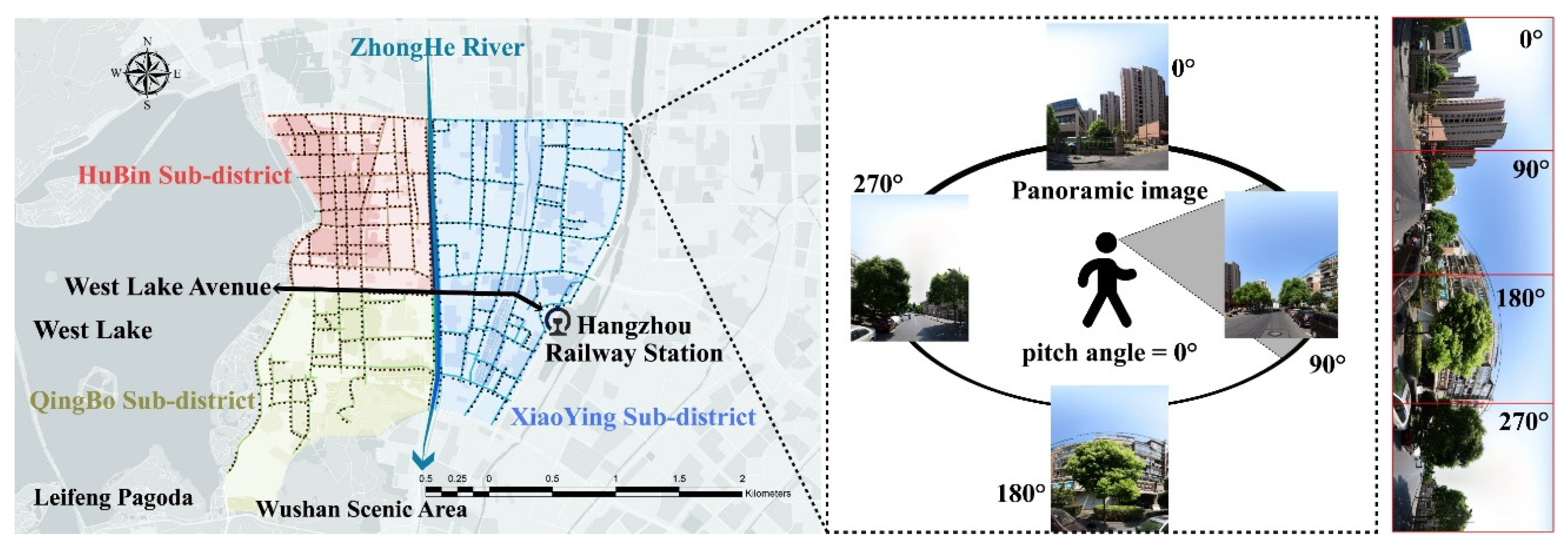
2.1. Study Areas
2.2. Data Preparation
3. Methods
3.1. Quantification of the VPIQ Measure
3.1.1. Form
3.1.2. Line
3.1.3. Texture
3.1.4. Color
3.2. Exploring Spatial Variation Using VPIQ in Street Space
3.2.1. Visual Variation in the Overall Single Street Space
3.2.2. Visual Variation within a Single Street Space
3.2.3. The Relevance of Spatial Variation to Street Elements
3.3. Exploring the Factors Influencing the Correlation between Spatial Information Values and Street Elements
3.3.1. Geographically Weighted Regression
3.3.2. Selection and Implementation of Independent Variables
4. Results
4.1. Results of the Spatial Variation of Streets Measured Using VPIQ
4.1.1. Overall Performance of the Single Street VPIQ
4.1.2. Internal Performance of the Single Street VPIQ
4.1.3. Coupling Results
4.2. Analysis of Factors Influencing the Value of Spatial Information
4.2.1. OLS Results
4.2.2. GWR Results
5. Discussion
5.1. Interpretation and Significance of Spatial Variation Measured with VPIQ
5.2. Significance and Application of Factors Affecting VPIQ
5.3. Summary
6. Conclusions
Author Contributions
Funding
Institutional Review Board Statement
Informed Consent Statement
Data Availability Statement
Conflicts of Interest
Appendix A. Illustration of Quantization Methods for Occlusion and Segmentation

Appendix B. Image Brightness Correction Display

References
- Biljecki, F.; Ito, K. Street View Imagery in Urban Analytics and GIS: A Review. Landsc. Urban Plan. 2021, 215, 104217. [Google Scholar] [CrossRef]
- Dong, R.; Zhang, Y.; Zhao, J. How Green Are the Streets Within the Sixth Ring Road of Beijing? An Analysis Based on Tencent Street View Pictures and the Green View Index. Int. J. Environ. Res. Public Health 2018, 15, 1367. [Google Scholar] [CrossRef] [PubMed] [Green Version]
- Wu, J.; Cheng, L.; Chu, S.; Xia, N.; Li, M. A Green View Index for Urban Transportation: How Much Greenery Do We View While Moving around in Cities? Int. J. Sustain. Transp. 2020, 14, 972–989. [Google Scholar] [CrossRef]
- Steinmetz-Wood, M.; Velauthapillai, K.; O’Brien, G.; Ross, N.A. Assessing the Micro-Scale Environment Using Google Street View: The Virtual Systematic Tool for Evaluating Pedestrian Streetscapes (Virtual-STEPS). BMC Public Health 2019, 19, 1246. [Google Scholar] [CrossRef] [PubMed] [Green Version]
- Zhou, Z.; Xu, Z. Detecting the Pedestrian Shed and Walking Route Environment of Urban Parks with Open-Source Data: A Case Study in Nanjing, China. Int. J. Environ. Res. Public Health 2020, 17, 4826. [Google Scholar] [CrossRef]
- Hu, C.-B.; Zhang, F.; Gong, F.-Y.; Ratti, C.; Li, X. Classification and Mapping of Urban Canyon Geometry Using Google Street View Images and Deep Multitask Learning. Build. Environ. 2020, 167, 106424. [Google Scholar] [CrossRef]
- Khamchiangta, D.; Dhakal, S. Physical and Non-Physical Factors Driving Urban Heat Island: Case of Bangkok Metropolitan Administration, Thailand. J. Environ. Manag. 2019, 248, 109285. [Google Scholar] [CrossRef]
- Li, Z.; Long, Y. Analysis of the Variation in Quality of Street Space in Shrinking Cities Based on Dynamic Street View Picture Recognition: A Case Study of Qiqihar. In Shrinking Cities in China: The Other Facet of Urbanization; The Urban Book Series; Long, Y., Gao, S., Eds.; Springer: Singapore, 2019; pp. 141–155. ISBN 9789811326462. [Google Scholar]
- Ye, Y.; Zeng, W.; Shen, Q.; Zhang, X.; Lu, Y. The Visual Quality of Streets: A Human-Centred Continuous Measurement Based on Machine Learning Algorithms and Street View Images. Environ. Plan. B Urban Anal. City Sci. 2019, 46, 1439–1457. [Google Scholar] [CrossRef]
- Chiang, Y.-C.; Li, D.; Jane, H.-A. Wild or Tended Nature? The Effects of Landscape Location and Vegetation Density on Physiological and Psychological Responses. Landsc. Urban Plan. 2017, 167, 72–83. [Google Scholar] [CrossRef]
- Gao, T.; Zhang, T.; Zhu, L.; Gao, Y.; Qiu, L. Exploring Psychophysiological Restoration and Individual Preference in the Different Environments Based on Virtual Reality. Int. J. Environ. Res. Public Health 2019, 16, 3102. [Google Scholar] [CrossRef]
- Jo, H.I.; Jeon, J.Y. Overall Environmental Assessment in Urban Parks: Modelling Audio-Visual Interaction with a Structural Equation Model Based on Soundscape and Landscape Indices. Build. Environ. 2021, 204, 108166. [Google Scholar] [CrossRef]
- Petucco, C.; Skovsgaard, J.P.; Jensen, F.S. Recreational Preferences Depending on Thinning Practice in Young Even-Aged Stands of Pedunculate Oak (Quercus robur L.): Comparing the Opinions of Forest and Landscape Experts and the General Population of Denmark. Scand. J. For. Res. 2013, 28, 668–676. [Google Scholar] [CrossRef]
- Wartmann, F.M.; Frick, J.; Kienast, F.; Hunziker, M. Factors Influencing Visual Landscape Quality Perceived by the Public. Results from a National Survey. Landsc. Urban Plan. 2021, 208, 104024. [Google Scholar] [CrossRef]
- Sharifi, A.; Allam, Z. On the Taxonomy of Smart City Indicators and Their Alignment with Sustainability and Resilience. Environ. Plan. B Urban Anal. City Sci. 2022, 49, 1536–1555. [Google Scholar] [CrossRef]
- Cugurullo, F. Exposing Smart Cities and Eco-Cities: Frankenstein Urbanism and the Sustainability Challenges of the Experimental City. Environ. Plan. A 2018, 50, 73–92. [Google Scholar] [CrossRef] [Green Version]
- Sharifi, A.; Allam, Z.; Feizizadeh, B.; Ghamari, H. Three Decades of Research on Smart Cities: Mapping Knowledge Structure and Trends. Sustainability 2021, 13, 7140. [Google Scholar] [CrossRef]
- Yigitcanlar, T.; Cugurullo, F. The Sustainability of Artificial Intelligence: An Urbanistic Viewpoint from the Lens of Smart and Sustainable Cities. Sustainability 2020, 12, 8548. [Google Scholar] [CrossRef]
- Qayyum, S.; Ullah, F.; Al-Turjman, F.; Mojtahedi, M. Managing Smart Cities through Six Sigma DMADICV Method: A Review-Based Conceptual Framework. Sustain. Cities Soc. 2021, 72, 103022. [Google Scholar] [CrossRef]
- Kim, J.H.; Lee, S.; Hipp, J.R.; Ki, D. Decoding Urban Landscapes: Google Street View and Measurement Sensitivity. Comput. Environ. Urban Syst. 2021, 88, 101626. [Google Scholar] [CrossRef]
- Xue, F.; Li, X.; Lu, W.; Webster, C.J.; Chen, Z.; Lin, L. Big Data-Driven Pedestrian Analytics: Unsupervised Clustering and Relational Query Based on Tencent Street View Photographs. ISPRS Int. J. Geo-Inf. 2021, 10, 561. [Google Scholar] [CrossRef]
- Zhou, H.; He, S.; Cai, Y.; Wang, M.; Su, S. Social Inequalities in Neighborhood Visual Walkability: Using Street View Imagery and Deep Learning Technologies to Facilitate Healthy City Planning. Sustain. Cities Soc. 2019, 50, 101605. [Google Scholar] [CrossRef]
- Ullah, Z.; Al-Turjman, F.; Mostarda, L.; Gagliardi, R. Applications of Artificial Intelligence and Machine Learning in Smart Cities. Comput. Commun. 2020, 154, 313–323. [Google Scholar] [CrossRef]
- Cugurullo, F. Urban Artificial Intelligence: From Automation to Autonomy in the Smart City. Front. Sustain. Cities 2020, 2, 38. [Google Scholar] [CrossRef]
- Allam, Z.; Dhunny, Z.A. On Big Data, Artificial Intelligence and Smart Cities. Cities 2019, 89, 80–91. [Google Scholar] [CrossRef]
- Wang, M.; Vermeulen, F. Life between Buildings from a Street View Image: What Do Big Data Analytics Reveal about Neighbourhood Organisational Vitality? Urban Stud. 2021, 58, 3118–3139. [Google Scholar] [CrossRef]
- Zhao, T.; Liang, X.; Tu, W.; Huang, Z.; Biljecki, F. Sensing Urban Soundscapes from Street View Imagery. Comput. Environ. Urban Syst. 2023, 99, 101915. [Google Scholar] [CrossRef]
- Wang, M.; Chen, Z.; Rong, H.H.; Mu, L.; Zhu, P.; Shi, Z. Ridesharing Accessibility from the Human Eye: Spatial Modeling of Built Environment with Street-Level Images. Comput. Environ. Urban Syst. 2022, 97, 101858. [Google Scholar] [CrossRef]
- Inoue, T.; Manabe, R.; Murayama, A.; Koizumi, H. Landscape Value in Urban Neighborhoods: A Pilot Analysis Using Street-Level Images. Landsc. Urban Plan. 2022, 221, 104357. [Google Scholar] [CrossRef]
- Larkin, A.; Gu, X.; Chen, L.; Hystad, P. Predicting Perceptions of the Built Environment Using GIS, Satellite and Street View Image Approaches. Landsc. Urban Plan. 2021, 216, 104257. [Google Scholar] [CrossRef]
- Verma, D.; Jana, A.; Ramamritham, K. Machine-Based Understanding of Manually Collected Visual and Auditory Datasets for Urban Perception Studies. Landsc. Urban Plan. 2019, 190, 103604. [Google Scholar] [CrossRef]
- Chen, C.; Li, H.; Luo, W.; Xie, J.; Yao, J.; Wu, L.; Xia, Y. Predicting the Effect of Street Environment on Residents’ Mood States in Large Urban Areas Using Machine Learning and Street View Images. Sci. Total Environ. 2022, 816, 151605. [Google Scholar] [CrossRef]
- Li, X.; Cai, B.Y.; Ratti, C. Using Street-Level Images and Deep Learning for Urban La Ndscape STUDIES. Landsc. Archit. Front. 2018, 6, 20. [Google Scholar] [CrossRef] [Green Version]
- Xia, Y.; Yabuki, N.; Fukuda, T. Development of a System for Assessing the Quality of Urban Street-Level Greenery Using Street View Images and Deep Learning. Urban For. Urban Green. 2021, 59, 126995. [Google Scholar] [CrossRef]
- Zhang, F.; Zhang, D.; Liu, Y.; Lin, H. Representing Place Locales Using Scene Elements. Comput. Environ. Urban Syst. 2018, 71, 153–164. [Google Scholar] [CrossRef]
- Han, J.M.; Lee, N. Holistic Visual Data Representation for Built Environment Assessment. Int. J. SDP 2018, 13, 516–527. [Google Scholar] [CrossRef]
- Zhang, F.; Wu, L.; Zhu, D.; Liu, Y. Social Sensing from Street-Level Imagery: A Case Study in Learning Spatio-Temporal Urban Mobility Patterns. ISPRS J. Photogramm. Remote Sens. 2019, 153, 48–58. [Google Scholar] [CrossRef]
- Verma, D.; Jana, A.; Ramamritham, K. Predicting Human Perception of the Urban Environment in a Spatiotemporal Urban Setting Using Locally Acquired Street View Images and Audio Clips. Build. Environ. 2020, 186, 107340. [Google Scholar] [CrossRef]
- Cheng, L.; Chu, S.; Zong, W.; Li, S.; Wu, J.; Li, M. Use of Tencent Street View Imagery for Visual Perception of Streets. ISPRS Int. J. Geo-Inf. 2017, 6, 265. [Google Scholar] [CrossRef] [Green Version]
- Fu, Y.; Song, Y. Evaluating Street View Cognition of Visible Green Space in Fangcheng District of Shenyang with the Green View Index. In Proceedings of the 2020 Chinese Control And Decision Conference (CCDC), Hefei, China, 22–24 August 2020; pp. 144–148. [Google Scholar]
- Wang, R.; Liu, Y.; Lu, Y.; Yuan, Y.; Zhang, J.; Liu, P.; Yao, Y. The Linkage between the Perception of Neighbourhood and Physical Activity in Guangzhou, China: Using Street View Imagery with Deep Learning Techniques. Int. J. Health Geogr. 2019, 18, 18. [Google Scholar] [CrossRef]
- Zhang, L.; Ye, Y.; Zeng, W.; Chiaradia, A. A Systematic Measurement of Street Quality through Multi-Sourced Urban Data: A Human-Oriented Analysis. Int. J. Environ. Res. Public Health 2019, 16, 1782. [Google Scholar] [CrossRef]
- Du, K.; Ning, J.; Yan, L. How Long Is the Sun Duration in a Street Canyon?—Analysis of the View Factors of Street Canyons. Build. Environ. 2020, 172, 106680. [Google Scholar] [CrossRef]
- Wu, B.; Yu, B.; Shu, S.; Liang, H.; Zhao, Y.; Wu, J. Mapping Fine-Scale Visual Quality Distribution inside Urban Streets Using Mobile LiDAR Data. Build. Environ. 2021, 206, 108323. [Google Scholar] [CrossRef]
- Yao, Y.; Wang, J.; Hong, Y.; Qian, C.; Guan, Q.; Liang, X.; Dai, L.; Zhang, J. Discovering the Homogeneous Geographic Domain of Human Perceptions from Street View Images. Landsc. Urban Plan. 2021, 212, 104125. [Google Scholar] [CrossRef]
- Wu, C.; Peng, N.; Ma, X.; Li, S.; Rao, J. Assessing Multiscale Visual Appearance Characteristics of Neighbourhoods Using Geographically Weighted Principal Component Analysis in Shenzhen, China. Comput. Environ. Urban Syst. 2020, 84, 101547. [Google Scholar] [CrossRef]
- Yang, L.; Yu, K.; Ai, J.; Liu, Y.; Yang, W.; Liu, J. Dominant Factors and Spatial Heterogeneity of Land Surface Temperatures in Urban Areas: A Case Study in Fuzhou, China. Remote Sens. 2022, 14, 1266. [Google Scholar] [CrossRef]
- Gong, F.-Y.; Zeng, Z.-C.; Zhang, F.; Li, X.; Ng, E.; Norford, L.K. Mapping Sky, Tree, and Building View Factors of Street Canyons in a High-Density Urban Environment. Build. Environ. 2018, 134, 155–167. [Google Scholar] [CrossRef]
- Liang, J.; Gong, J.; Zhang, J.; Li, Y.; Wu, D.; Zhang, G. GSV2SVF-an Interactive GIS Tool for Sky, Tree and Building View Factor Estimation from Street View Photographs. Build. Environ. 2020, 168, 106475. [Google Scholar] [CrossRef]
- Szcześniak, J.T.; Ang, Y.Q.; Letellier-Duchesne, S.; Reinhart, C.F. A Method for Using Street View Imagery to Auto-Extract Window-to-Wall Ratios and Its Relevance for Urban-Level Daylighting and Energy Simulations. Build. Environ. 2022, 207, 108108. [Google Scholar] [CrossRef]
- Daniel, T.C.; Vining, J. Methodological Issues in the Assessment of Landscape Quality. In Behavior and the Natural Environment; Altman, I., Wohlwill, J.F., Eds.; Human Behavior and, Environment; Springer: Boston, MA, USA, 1983; pp. 39–84. ISBN 978-1-4613-3539-9. [Google Scholar]
- Litton, R.B. Forest Landscape Description and Inventories: A Basis for Planning and Design; USDA Forest Service Research Paper DSW-49; Paciffic Southwest Forest and Range Expertment Station: Berkeley, CA, USA, 1968.
- Daniel, T.C. Measuring the Quality of the Natural Environment: A Psychophysical Approach. Am. Psychol. 1990, 45, 633–637. [Google Scholar] [CrossRef]
- Bin, J.; Gardiner, B.; Li, E.; Liu, Z. Multi-Source Urban Data Fusion for Property Value Assessment: A Case Study in Philadelphia. Neurocomputing 2020, 404, 70–83. [Google Scholar] [CrossRef]
- Najafizadeh, L.; Froehlich, J.E. A Feasibility Study of Using Google Street View and Computer Vision to Track the Evolution of Urban Accessibility. In Proceedings of the 20th International ACM SIGACCESS Conference on Computers and Accessibility, Galway, Ireland, 22–24 October 2018; Association for Computing Machinery: New York, NY, USA, 2018; pp. 340–342. [Google Scholar]
- Novack, T.; Vorbeck, L.; Lorei, H.; Zipf, A. Towards Detecting Building Facades with Graffiti Artwork Based on Street View Images. ISPRS Int. J. Geo-Inf. 2020, 9, 98. [Google Scholar] [CrossRef] [Green Version]
- Cooper, J.; Oskrochi, R. Fractal Analysis of Street Vistas: A Potential Tool for Assessing Levels of Visual Variety in Everyday Street Scenes. Environ. Plan. B Plan. Des. 2008, 35, 349–363. [Google Scholar] [CrossRef] [Green Version]
- Ma, L.; Zhang, H.; Lu, M. Building’s Fractal Dimension Trend and Its Application in Visual Complexity Map. Build. Environ. 2020, 178, 106925. [Google Scholar] [CrossRef]
- Brink, A.D. Using Spatial Information as an Aid to Maximum Entropy Image Threshold Selection. Pattern Recognit. Lett. 1996, 17, 29–36. [Google Scholar] [CrossRef]
- Silva, L.E.V.; Duque, J.J.; Felipe, J.C.; Murta, L.O., Jr.; Humeau-Heurtier, A. Two-Dimensional Multiscale Entropy Analysis: Applications to Image Texture Evaluation. Signal Process. 2018, 147, 224–232. [Google Scholar] [CrossRef]
- Zunino, L.; Ribeiro, H.V. Discriminating Image Textures with the Multiscale Two-Dimensional Complexity-Entropy Causality Plane. Chaos Solitons Fractals 2016, 91, 679–688. [Google Scholar] [CrossRef] [Green Version]
- Han, J. A Visual Evaluation Study for Walking Streetscape. Ph.D. Thesis, Southwest Jiaotong University, Chengdu, China, 2018. [Google Scholar]
- Jain, A.K. Data Clustering: 50 Years beyond K-Means. Pattern Recognit. Lett. 2010, 31, 651–666. [Google Scholar] [CrossRef]
- Cadenasso, M.L.; Pickett, S.T.A.; Schwarz, K. Spatial Heterogeneity in Urban Ecosystems: Reconceptualizing Land Cover and a Framework for Classification. Front. Ecol. Environ. 2007, 5, 80–88. [Google Scholar] [CrossRef]
- Li, A.; Zhao, P.; Huang, Y.; Gao, K.; Axhausen, K.W. An Empirical Analysis of Dockless Bike-Sharing Utilization and Its Explanatory Factors: Case Study from Shanghai, China. J. Transp. Geogr. 2020, 88, 102828. [Google Scholar] [CrossRef]
- Ma, X.; Ma, C.; Wu, C.; Xi, Y.; Yang, R.; Peng, N.; Zhang, C.; Ren, F. Measuring Human Perceptions of Streetscapes to Better Inform Urban Renewal: A Perspective of Scene Semantic Parsing. Cities 2021, 110, 103086. [Google Scholar] [CrossRef]
- Yang, H.; Fu, M.; Wang, L.; Tang, F. Mixed Land Use Evaluation and Its Impact on Housing Prices in Beijing Based on Multi-Source Big Data. Land 2021, 10, 1103. [Google Scholar] [CrossRef]
- Edquist, J.; Rudin-Brown, C.M.; Lenné, M.G. The Effects of On-Street Parking and Road Environment Visual Complexity on Travel Speed and Reaction Time. Accid. Anal. Prev. 2012, 45, 759–765. [Google Scholar] [CrossRef] [PubMed]


| The Importance of Bi Compared to Bj | Absolutely Important | Very Important | Comparatively Important | Slightly Important | Same Important | Slightly Minor | Comparatively Minor | Very Minor | Absolutely Minor |
|---|---|---|---|---|---|---|---|---|---|
| aij | 9 | 7 | 5 | 3 | 1 | 1/3 | 1/5 | 1/7 | 1/9 |
| Street Elements | POI Data | |||
|---|---|---|---|---|
| Original Categories | Simplified Categories | Original Categories | Simplified Categories | |
| Reserved Variables | Building | Building_A | Transportation Facilities | Transportation |
| Vegetation | Vegetation_A | Road | ||
| Sky | Sky_A | Car Service | ||
| Pole | Infrustructure_A | Hotels | Residence | |
| Traffic light | Real estate communities | |||
| Traffic sign | Recreation | Entertainment | ||
| Fence | Restaurants | |||
| Wall | Barrier_A | Tourist Attractions | ||
| Terrain | Shopping | |||
| Road | Road_A | Life Services | Life | |
| Sidewalk | Company | Public | ||
| Finance | ||||
| Business Building | ||||
| Medical | ||||
| Government Agencies | ||||
| Excluded variables | Person, Rider, Car, Truck, Bus, Train, Motorcycle, Bicycle | |||
| Target Layer | Criterion Layers and Weights | Scheme Layers and Weights | ||
|---|---|---|---|---|
| Hc_SUM | Form information | 0.355 | HCB | 0.304 |
| HCO | 0.051 | |||
| Line information | 0.145 | HLI | 0.145 | |
| Texture information | 0.145 | HTE | 0.145 | |
| Color information | 0.355 | Hc_B | 0.030 | |
| Hc_C | 0.091 | |||
| Hc_G | 0.170 | |||
| Hc_M | 0.011 | |||
| Hc_R | 0.023 | |||
| Hc_Y | 0.030 | |||
| Independent Variable | Description | OLS | GWR | |||||||
|---|---|---|---|---|---|---|---|---|---|---|
| Coef | t | p | VIF | Mean | std | 25% | Median | 75% | ||
| Building_A | The proportion of architectural elements in the picture | −0.043 | −0.675 | 0.500 | 1.627 | −0.070 | 0.275 | −0.469 | −0.082 | 0.287 |
| Vegetation_A | The proportion of vegetation elements in the picture | −1.017 | −28.881 | 0.000 *** | 1.405 | −1.077 | 0.152 | −1.368 | −1.089 | −0.827 |
| Hc_LA | The degree of mixing of business functions around the sampling point | −0.025 | −2.766 | 0.006 ** | 1.004 | −0.017 | 0.035 | −0.044 | −0.019 | 0.011 |
| Infrustructure_A | pole, traffic light, traffic sign, fence elements take up the proportion of the picture | −0.975 | −3.059 | 0.002 ** | 1.031 | −1.325 | 1.431 | −2.699 | −1.280 | 0.159 |
| Barrier_A | wall, terrain elements take up the proportion of the picture | −1.099 | −4.745 | 0.000 *** | 1.211 | −0.096 | 1.092 | −0.901 | −0.149 | 0.754 |
| Road_A | road, sidewalk elements take up the proportion of the picture | −1.186 | −6.331 | 0.000 *** | 1.262 | −1.357 | 0.782 | −2.055 | −1.430 | −0.780 |
| Constants | 2.047 | 54.351 | 0.000 *** | |||||||
| R2 | 0.534 | R2 | 0.736 | |||||||
| Adjusted R² | 0.532 | Adjusted R2 | 0.710 | |||||||
| AICc | −3926 | AICc | −9780 | |||||||
| Name | Description |
|---|---|
| HCB | Form information quantity |
| HLI | Line information quantity |
| the | Texture information quantity |
| Hc | Color information quantity |
| VPIQ | HCB, HCO, HLtheHTE, Hc (Hc_G, Hc_M, Hc_R, Hc_Y, Hc_B, and Hc_C) |
| Hc_SUM | The total value of visual perception information quantity (VPIQ) based on Fuzzy Comprehensive Evaluation (FCE) |
| SCV | The fluctuation range of Hc_SUM in a street |
| HCK | K-means clustering is performed based on 10 VPIQ indicators, and the diversity of clustering categories in each street is calculated |
| Sum_avg | The average value of Hc_SUM in each street |
| RLS | Relative length of streets |
Publisher’s Note: MDPI stays neutral with regard to jurisdictional claims in published maps and institutional affiliations. |
© 2022 by the authors. Licensee MDPI, Basel, Switzerland. This article is an open access article distributed under the terms and conditions of the Creative Commons Attribution (CC BY) license (https://creativecommons.org/licenses/by/4.0/).
Share and Cite
Liu, Z.; Ma, X.; Hu, L.; Lu, S.; Ye, X.; You, S.; Tan, Z.; Li, X. Information in Streetscapes—Research on Visual Perception Information Quantity of Street Space Based on Information Entropy and Machine Learning. ISPRS Int. J. Geo-Inf. 2022, 11, 628. https://doi.org/10.3390/ijgi11120628
Liu Z, Ma X, Hu L, Lu S, Ye X, You S, Tan Z, Li X. Information in Streetscapes—Research on Visual Perception Information Quantity of Street Space Based on Information Entropy and Machine Learning. ISPRS International Journal of Geo-Information. 2022; 11(12):628. https://doi.org/10.3390/ijgi11120628
Chicago/Turabian StyleLiu, Ziyi, Xinyao Ma, Lihui Hu, Shan Lu, Xiaomin Ye, Shuhang You, Zhe Tan, and Xin Li. 2022. "Information in Streetscapes—Research on Visual Perception Information Quantity of Street Space Based on Information Entropy and Machine Learning" ISPRS International Journal of Geo-Information 11, no. 12: 628. https://doi.org/10.3390/ijgi11120628
APA StyleLiu, Z., Ma, X., Hu, L., Lu, S., Ye, X., You, S., Tan, Z., & Li, X. (2022). Information in Streetscapes—Research on Visual Perception Information Quantity of Street Space Based on Information Entropy and Machine Learning. ISPRS International Journal of Geo-Information, 11(12), 628. https://doi.org/10.3390/ijgi11120628