
An Effective Fingerprint-Based Indoor Positioning Algorithm Based on Extreme Values


Abstract
:1. Introduction
2. Related Work
3. Preliminaries and Framework of Proposed Algorithm
3.1. Subsection Problem Description
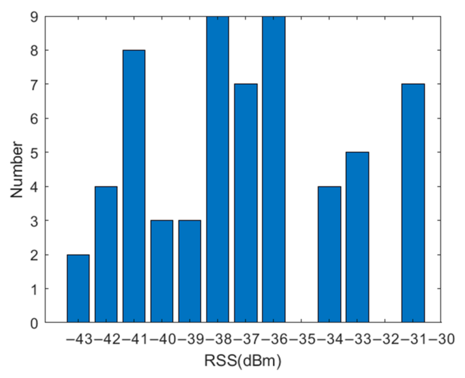
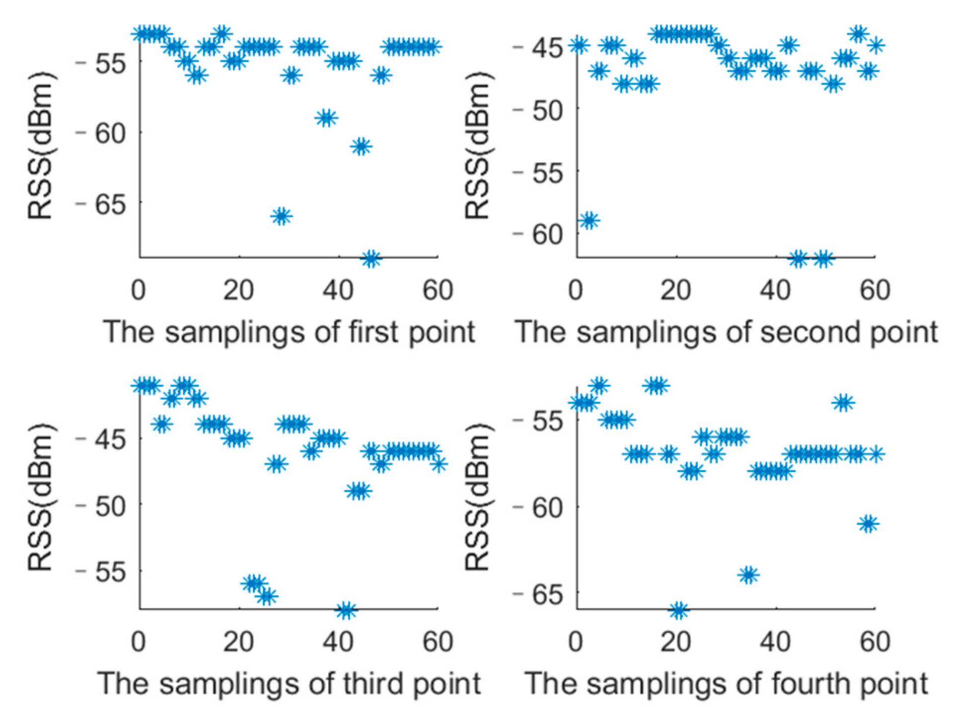
3.2. Preliminary Experiment
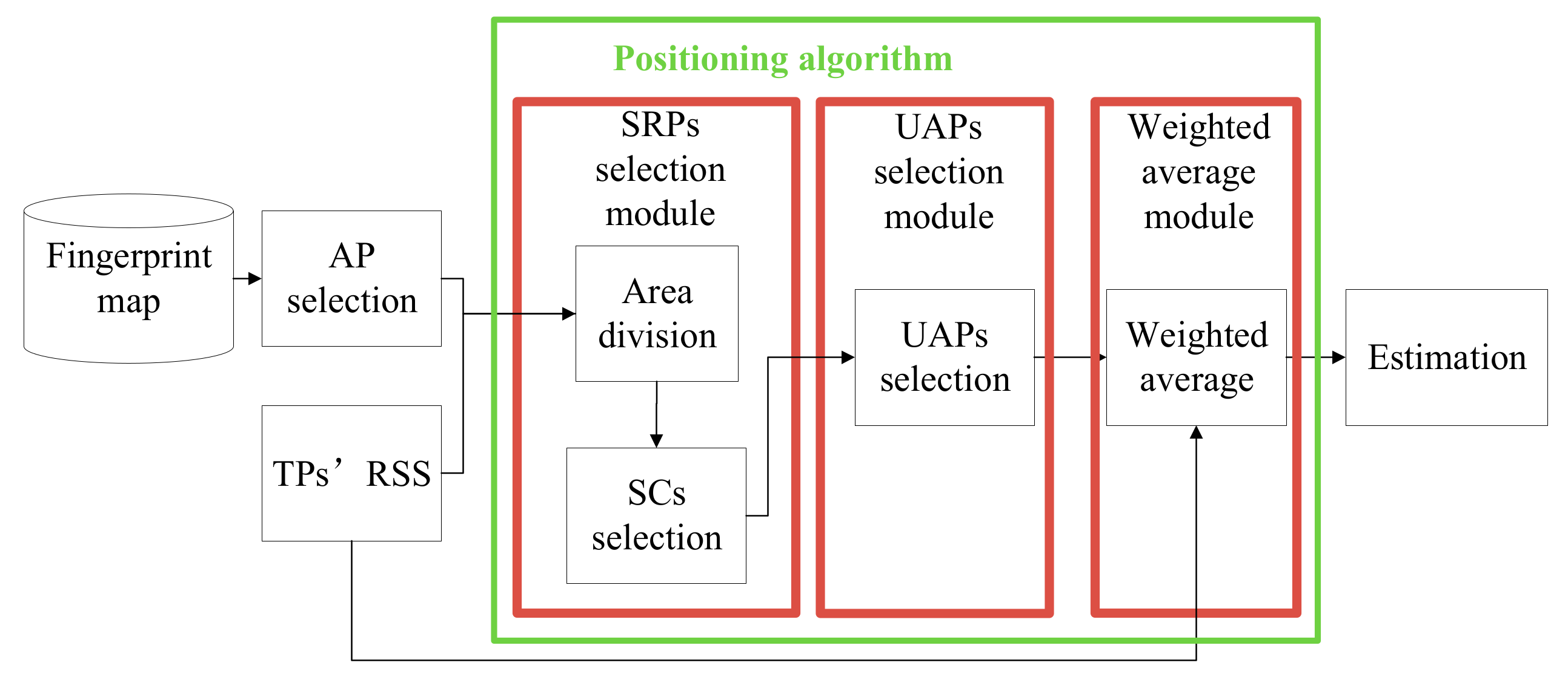
3.3. Framework
4. Algorithms
4.1. AP Selection Algorithm
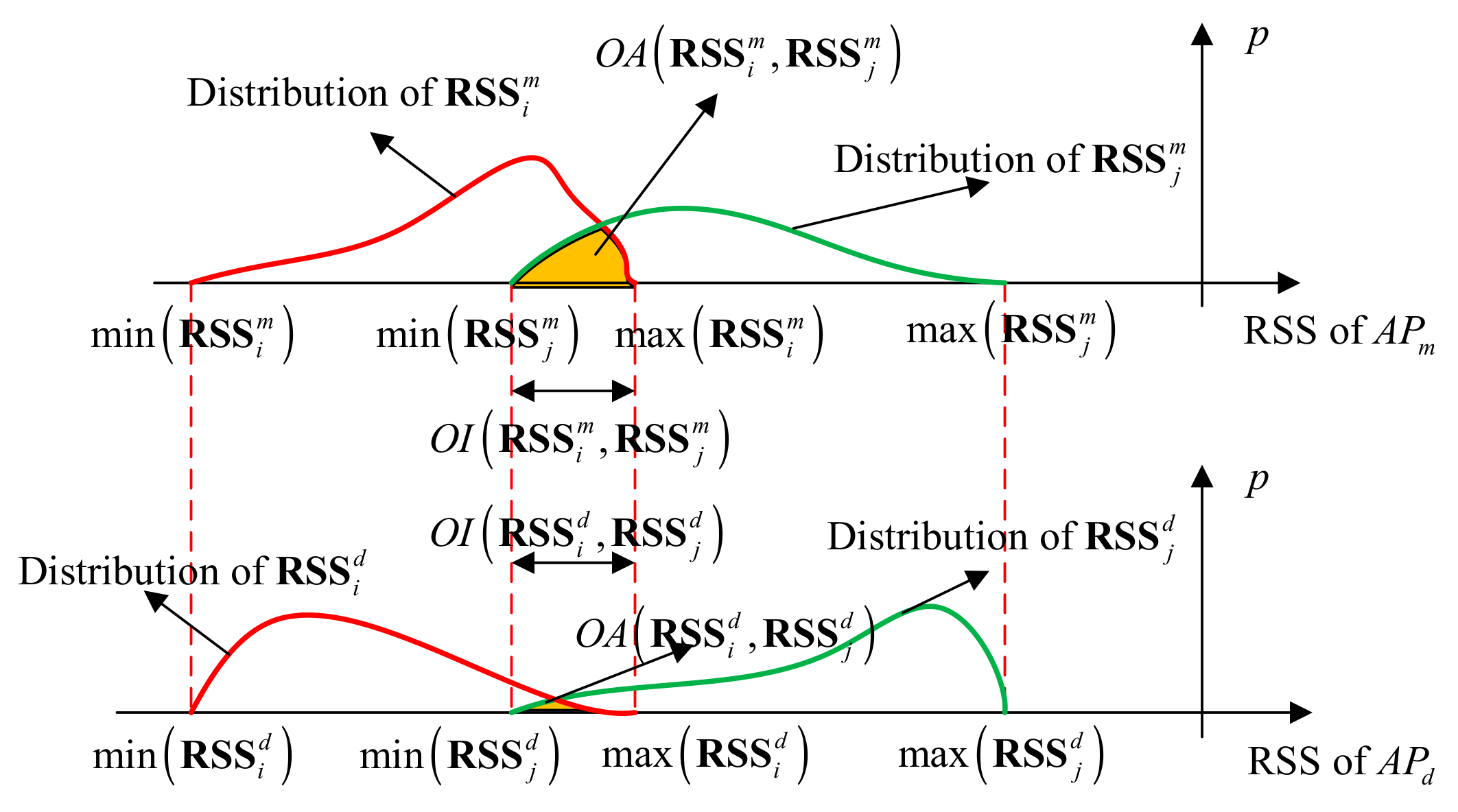
4.1.1. IOD Algorithm
4.1.2. Issue Statement of the IOD Algorithm
4.1.3. The Proposed DIOD Algorithm
4.2. Positioning Algorithm
4.2.1. SRPs Selection Module
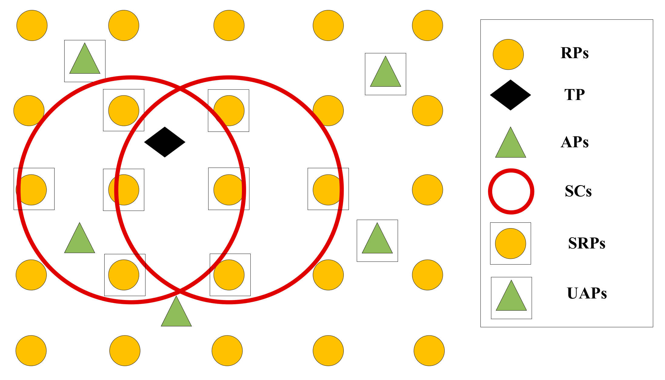
The RSS Extreme Values Collected at RPs in a Circle
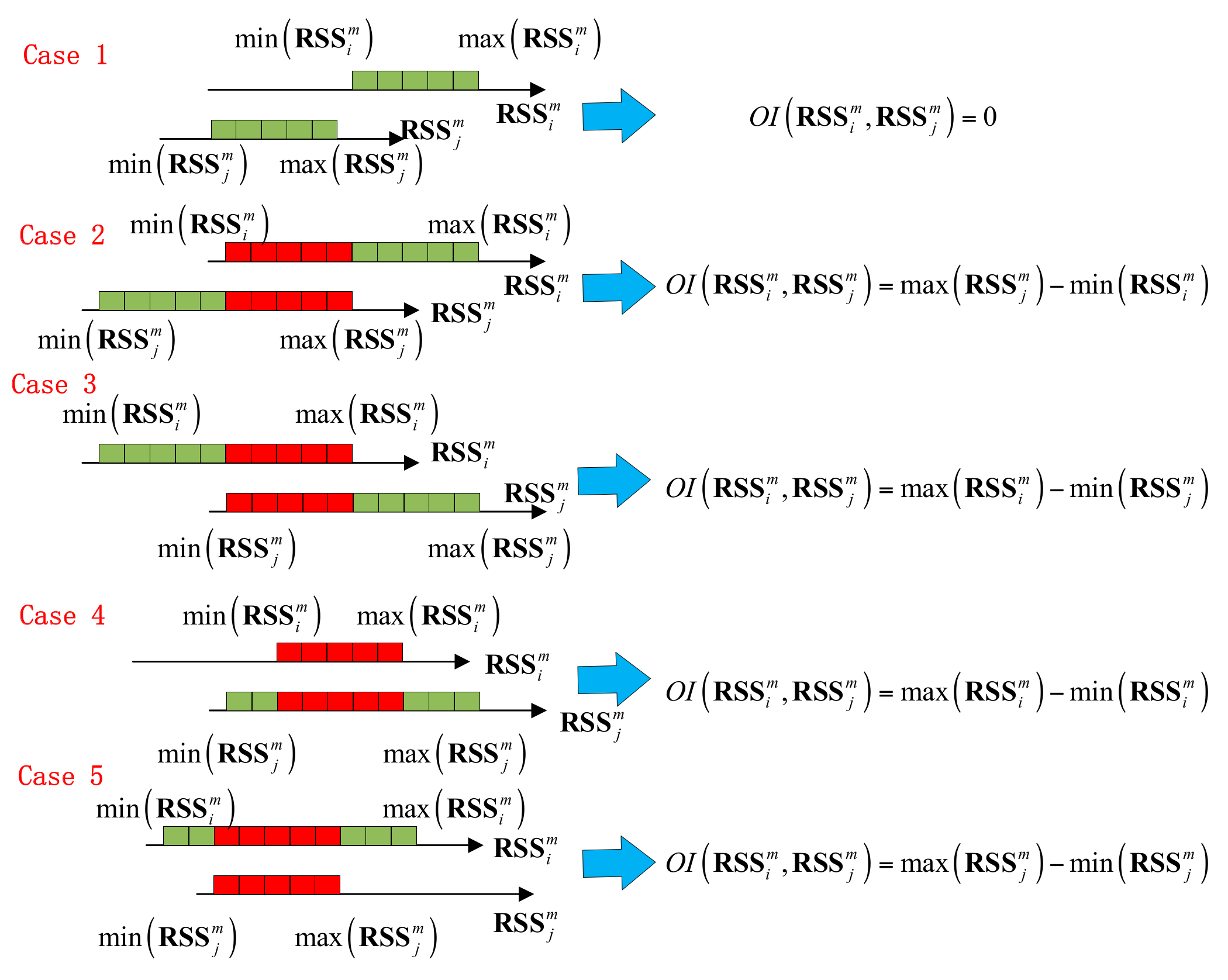
The SRPs Selection Criterion
4.2.2. UAPs Selection Module
4.2.3. Weighted Average Module
5. Experiments
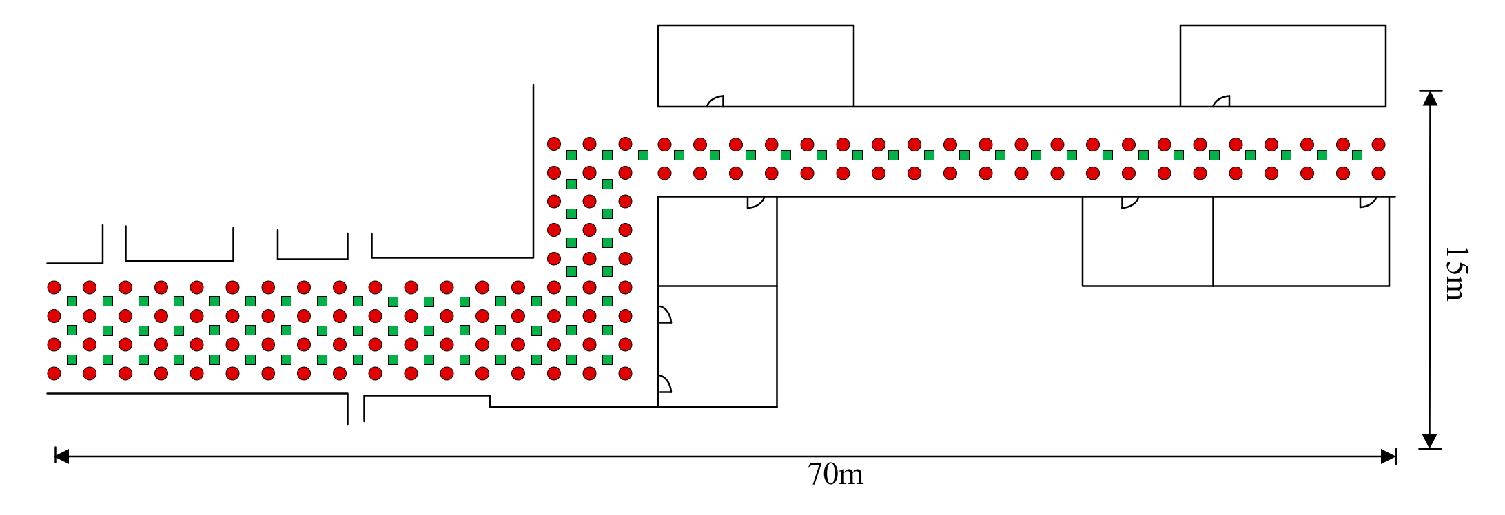
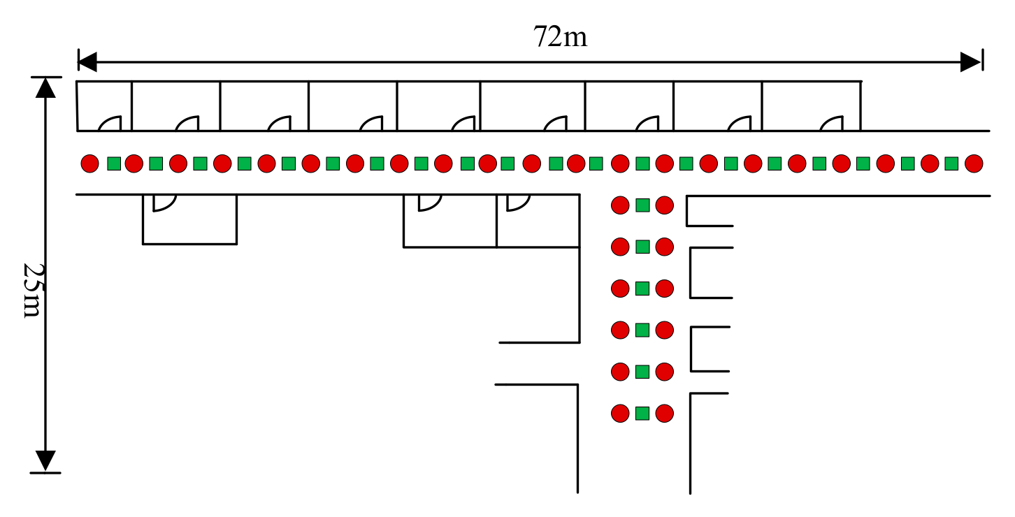
5.1. Experimental Settings
5.2. Comparison Algorithms and Performance Metric
5.3. Feasibility Evaluation
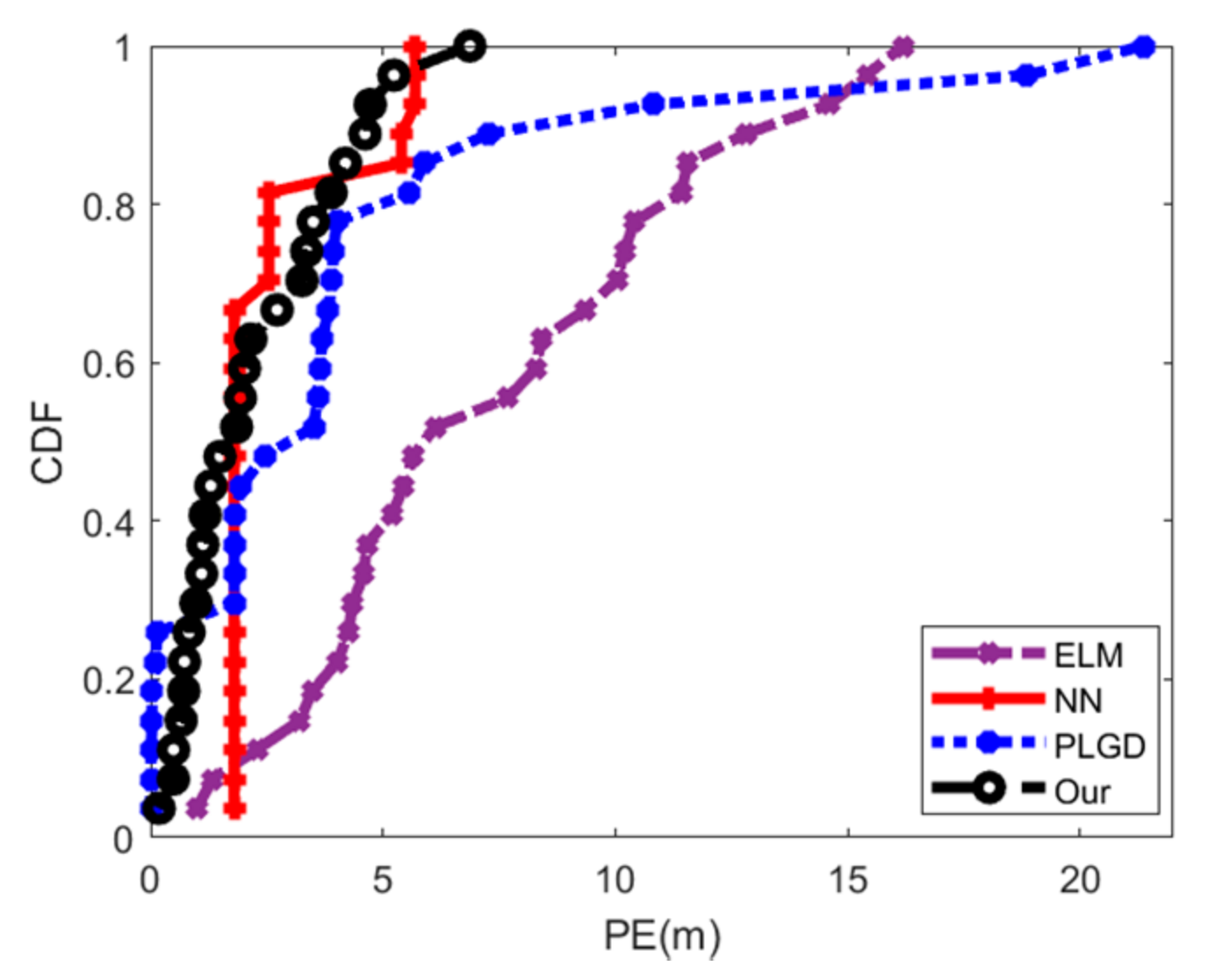
5.4. Positioning Accuracy Evaluation
5.5. Time Cost of Proposed Positioning Algorithm
6. Further Discussions
7. Conclusions
Author Contributions
Funding
Institutional Review Board Statement
Informed Consent Statement
Data Availability Statement
Acknowledgments
Conflicts of Interest
References
- Cao, H.; Wang, Y.; Bi, J.; Sun, M.; Qi, H.; Xu, S. Fingerprint Positioning Method for Dual-Band Wi-Fi Based on Gaussian Process Regression and K-Nearest Neighbor. ISPRS Int. J. Geo-Inf. 2021, 10, 706. [Google Scholar] [CrossRef]
- Bi, J.; Huang, L.; Cao, H.; Yao, G.; Sang, W.; Zhen, J.; Liu, Y. Improved Indoor Fingerprinting Localization Method Using Clustering Algorithm and Dynamic Compensation. ISPRS Int. J. Geo-Inf. 2021, 10, 613. [Google Scholar] [CrossRef]
- Farrell, J. Aided Navigation: GPS with High Rate Sensors; McGraw-Hill: New York, NY, USA, 2008. [Google Scholar]
- Kok, M.; Hol, J.; Schön, T. Indoor Positioning Using Ultrawideband and Inertial Measurements. IEEE Trans. Veh. Technol. 2015, 64, 1293–1303. [Google Scholar] [CrossRef] [Green Version]
- He, S.; Chan, S. Wi-fi fingerprint-based indoor positioning: Recent advances and comparisons. IEEE Commun. Surv. Tutor. 2016, 18, 466–490. [Google Scholar] [CrossRef]
- Bandara, U.; Hasegawa, M.; Inoue, M.; Morikawa, H.; Aoyama, T. Design and implementation of a Bluetooth signal strength based location sensing system. In Proceedings of the 2004 IEEE Radio and Wireless Conference, Atlanta, GA, USA, 22 September 2004; pp. 319–322. [Google Scholar]
- Kuo, Y.; Pannuto, P.; Dutta, P. Demo: Luxapose: Indoor Positioning with Mobile Phones and Visible Light. In Proceedings of the 20th Annual International Conference on Mobile Computing and Networking, Maui, HI, USA, 7–11 September 2014; ACM: New York, NY, USA; pp. 299–302. [Google Scholar]
- Tao, Y.; Zhao, L. A novel system for wifi radio map automatic adaptation and indoor positioning. IEEE Trans. Veh. Technol. 2018, 67, 10683–10692. [Google Scholar] [CrossRef]
- Chen, L.; Yang, K.; Wang, X. Robust Cooperative Wi-Fi Fingerprint-Based Indoor Localization. IEEE Internet Things J. 2016, 3, 1406–1417. [Google Scholar] [CrossRef]
- Youssef, M.; Agrawala, A. The Horus location determination system. Wirel. Netw. 2008, 14, 357–374. [Google Scholar] [CrossRef]
- Tao, Y.; Zhao, L. Fingerprint Localization with Adaptive Area Search. IEEE Commun. Lett. 2020, 24, 1446–1450. [Google Scholar] [CrossRef]
- Jun, J.; He, L.; Gu, Y.; Jiang, W.; Kushwaha, G.; Vipin, A.; Cheng, L.; Liu, C.; Zhu, T. Low-overhead WiFi fingerprinting. IEEE Trans. Mob. Comput. 2018, 17, 590–603. [Google Scholar] [CrossRef]
- Chen, P.; Shang, J.; Gu, F. Learning RSSI Feature via Ranking Model for Wi-Fi Fingerprinting Localization. IEEE Trans. Veh. Technol. 2020, 69, 1695–1705. [Google Scholar] [CrossRef]
- Zafari, F.; Gkelias, A.; Leung, K. A survey of indoor localization systems and technologies. IEEE Commun. Surv. Tutor. 2019, 21, 2568–2599. [Google Scholar] [CrossRef] [Green Version]
- Tang, L. Comparison of WiFi-Based Indoor Positioning Methods. In Proceedings of the 2019 13th International Conference on Signal Processing and Communication Systems (ICSPCS), Gold Coast, QLD, Australia, 16–18 December 2019; pp. 1–6. [Google Scholar]
- He, S.; Lin, W.; Chan, S. Indoor localization and automatic fingerprint update with altered AP signals. IEEE Trans. Mob. Comput. 2017, 16, 1897–1910. [Google Scholar] [CrossRef]
- Xue, M.; Sun, W.; Yu, H. Locate the Mobile Device by Enhancing the WiFi-Based Indoor Localization Model. IEEE Internet Things J. 2019, 6, 8792–8803. [Google Scholar] [CrossRef]
- Bahl, P.; Padmanabhan, V. RADAR: An In-Building RF-Based User Location and Tracking System. In Proceedings of the IEEE INFOCOM 2000, Tel Aviv, Israel, 26–30 March 2000; pp. 775–784. [Google Scholar]
- Yin, J.; Yang, Q.; Ni, L. Learning Adaptive Temporal Radio Maps for Signal-Strength-Based Location Estimation. IEEE Trans. Mob. Comput. 2008, 7, 869–883. [Google Scholar] [CrossRef] [Green Version]
- Hu, J.; Liu, D.; Yan, Z.; Liu, H. Experimental analysis on weight Knearest neighbor indoor fingerprint positioning. IEEE Internet Things J. 2019, 6, 891–897. [Google Scholar] [CrossRef]
- Xue, W.; Yu, K.; Hua, X.; Li, Q.; Qiu, W.; Zhou, B. APs’ virtual positions based reference point clustering and physical distance-based weighting for indoor Wi-Fi positioning. IEEE Internet Things J. 2018, 5, 3031–3042. [Google Scholar] [CrossRef]
- Shrestha, S.; Talvitie, J.; Lohan, E. Deconvolution-Based Indoor Localization with WLAN Signals and Unknown Access Point Locations. In Proceedings of the IEEE ICL-GNSS, Turin, Italy, 25–27 June 2013. [Google Scholar]
- Cramariuc, A.; Huttunen, H.; Lohan, E. Clustering Benefits in Mobile-Centric WiFi Positioning in multi-Floor Buildings. In Proceedings of the International Conference on Localization and GNSS (ICL-GNSS), Barcelona, Spain, 28–30 June 2016; pp. 1–6. [Google Scholar]
- Razavi, A.; Valkama, M.; Lohan, E.S. K-Means Fingerprint Clustering for Low-Complexity Floor Estimation in Indoor Mobile Localization. In Proceedings of the 2015 IEEE Globecom Workshops (GC Wkshps), San Diego, CA, USA, 6–10 December 2015; pp. 1–7. [Google Scholar]
- Hu, X.; Shang, J.; Gu, F.; Han, Q. Improving Wi-Fi indoor positioning via AP sets similarity and semi-supervised affinity propagation clustering. Int. J. Distrib. Sens. Netw. 2015, 2015, 109642. [Google Scholar] [CrossRef]
- Wang, B.; Liu, X.; Yu, B.; Jia, R.; Gan, X. An improved WiFi positioning method based on fingerprint clustering and signal weighted Euclidean distance. Sensors 2019, 19, 2300. [Google Scholar] [CrossRef] [Green Version]
- Abbas, M.; Elhamshary, M.; Rizk, H.; Torki, M.; Youssef, M. WiDeep: WiFi-Based Accurate and Robust Indoor Localization System Using Deep Learning. In Proceedings of the 2019 IEEE International Conference on Pervasive Computing and Communications (PerCom), Kyoto, Japan, 11–15 March 2019; pp. 1–10. [Google Scholar]
- Koike-Akino, T.; Wang, P.; Pajovic, M.; Sun, H.; Orlik, P.V. Fingerprinting-based indoor localization with commercial MMWave WiFi: A deep learning approach. IEEE Access 2020, 8, 84879–84892. [Google Scholar] [CrossRef]
- Lu, X.; Zou, H.; Zhou, H.; Xie, L.; Huang, G.-B. Robust Extreme Learning Machine with its Application to Indoor Positioning. IEEE Trans. Cybern. 2016, 46, 194–205. [Google Scholar] [CrossRef]
- Wu, B.; Ma, Z.; Poslad, S.; Zhang, W. An Efficient Wireless Access Point Selection Algorithm for Location Determination Based on RSSI Interval Overlap Degree Determination. In Proceedings of the 2018 Wireless Telecommunications Symposium (WTS), Phoenix, AZ, USA, 17–20 April 2018; pp. 1–8. [Google Scholar]
- Youssef, M.; Agrawala, A.; Udaya Shankar, A. WLAN Location Determination via Clustering and Probability Distributions. In Proceedings of the First IEEE International Conference on Pervasive Computing and Communications 2003 (PerCom 2003), Fort Worth, TX, USA, 26 March 2003; pp. 143–150. [Google Scholar]
- Zhang, W.; Yu, K.; Wang, W.; Li, X. A Self-Adaptive AP Selection Algorithm Based on Multi-Objective Optimization for Indoor WiFi Positioning. IEEE Internet Things J. 2021, 8, 1406–1416. [Google Scholar] [CrossRef]
- Chen, Y.; Yang, Q.; Yin, J.; Chai, X. Power-efficient access point selection for indoor location estimation. IEEE Trans. Knowl. Data Eng. 2016, 18, 877–888. [Google Scholar] [CrossRef] [Green Version]
- He, S.; Chan, S. Tilejunction: Mitigating signal noise for fingerprint-based indoor localization. IEEE Trans. Mob. Comput. 2016, 15, 1554–1568. [Google Scholar] [CrossRef]
- Lin, T.-N.; Fang, S.-H.; Tseng, W.-H.; Lee, C.-W.; Hsieh, J.-W. A group-discrimination-based access point selection for WLAN fingerprinting localization. IEEE Trans. Veh. Technol. 2014, 63, 3967–3976. [Google Scholar] [CrossRef]
- Zou, H.; Jin, M.; Jiang, H.; Xie, L.; Spanos, C.J. WinIPS: WiFi-based Non-intrusive Indoor Positioning System with Online Radio Map Construction and Adaptation. IEEE Trans. Wirel. Commun. 2017, 16, 8118–8130. [Google Scholar] [CrossRef]
- Huang, B.; Xu, Z.; Jia, B.; Mao, G. An online radio map update scheme for WiFi fingerprint-based localization. IEEE Internet Things J. 2019, 6, 6909–6918. [Google Scholar] [CrossRef]
- Wu, C.; Yang, Z.; Xiao, C. Automatic Radio Map Adaptation for Indoor Localization Using Smartphones. IEEE Trans. Mob. Comput. 2018, 17, 517–528. [Google Scholar] [CrossRef]
- Geladi, P.; Kowalski, B. Partial least-squares regression: A tutorial. Anal. Chim. Acta 1986, 185, 1–17. [Google Scholar] [CrossRef]
- Conti, A.; Dardari, D.; Guerra, M.; Mucchi, L.; Win, M.Z. Experimental characterization of diversity navigation. IEEE Syst. J. 2014, 8, 115–124. [Google Scholar] [CrossRef]
- Liu, Z.; Dai, W.; Win, M. Mercury: An infrastructure-free system for network localization and navigation. IEEE Trans. Mob. Comput. 2018, 17, 1119–1133. [Google Scholar] [CrossRef]
- Rai, A.; Chintalapudi, K.K.; Padmanabhan, V.N.; Sen, R. Zee: Zero-Effort Crowdsourcing for Indoor Localization. In Proceedings of the ACM 18th Annual International Conference on Mobile Computing and Networking, Istanbul, Turkey, 22–26 August 2012; pp. 293–304. [Google Scholar]
- Sun, W.; Liu, J.; Wu, C.; Yang, Z.; Zhang, X.; Liu, Y. MoLoc: On Distinguishing Fingerprint Twins. In Proceedings of the IEEE 33rd International Conference on Distributed Computing Systems, Philadelphia, PA, USA, 8–11 July 2013; pp. 226–235. [Google Scholar]
- Zhu, N.; Zhao, H.; Feng, W.; Wang, Z. A novel particle filter approach for indoor positioning by fusing WiFi and inertial sensors. Chin. J. Aeronaut. 2015, 28, 1725–1734. [Google Scholar] [CrossRef] [Green Version]
- Yang, S.; Dessai, P.; Verma, M.; Gerla, M. FreeLoc: Calibration-Free Crowdsourced Indoor Localization. In Proceedings of the 2013 IEEE INFOCOM, Turin, Italy, 14–19 April 2013; pp. 2481–2489. [Google Scholar]
- Xue, W.; Qiu, W.; Hua, X.; Yu, K. Improved Wi-Fi RSSI measurement for indoor localization. IEEE Sens. J. 2017, 17, 2224–2230. [Google Scholar] [CrossRef]
- Rappaport, T.S. Wireless Communications: Principles and Practice; Prentice-Hall: Englewood Cliffs, NJ, USA, 1996; Volume 2. [Google Scholar]
- Tao, Y.; Zhao, L. Fingerprint Localization with Circular Boundary. IEEE Commun. Lett. 2021, 25, 2928–2932. [Google Scholar] [CrossRef]


| Notations | Definition |
|---|---|
| N | Number of RPs |
| M | Number of APs |
| The RSS sampling of APm at RPn | |
| T | Number of samplings |
| The overlap length between and | |
| ρ | The length of the radius |
| Cn | The circle with RPn as center and ρ as the radius |
| fn | Number of RPs in Cn |
| The maximum RSS value of APm at RPs in Cn | |
| The minimum RSS value of APm at RPs in Cn | |
| RSS of APm at RPi in Cn in the tth second | |
| The whole minimum RSS value of APm in Cn | |
| The whole maximum RSS value of APm in Cm | |
| SCi | The ith similar circle (SC) |
| SCAPi | Unchanged APs in SCi |
| q | Largest number of unchanged APs |
| Similar Circle | Unchanged APs of each SC (SCAP) |
|---|---|
| sc1 | AP1, AP2, AP3, AP4, AP5, AP6, AP7 |
| sc2 | AP1, AP2, AP3, AP4, AP5, AP6, AP7 |
| sc3 | AP1, AP2, AP3, AP4, AP5, AP6, AP7 |
| sc4 | AP1, AP2, AP3, AP4, AP5, AP6, AP7 |
| sc5 | AP1, AP2, AP3, AP4, AP5, AP6, AP7 |
| sc6 | AP1, AP2, AP3, AP4, AP5, AP6, AP7 |
Publisher’s Note: MDPI stays neutral with regard to jurisdictional claims in published maps and institutional affiliations. |
© 2022 by the authors. Licensee MDPI, Basel, Switzerland. This article is an open access article distributed under the terms and conditions of the Creative Commons Attribution (CC BY) license (https://creativecommons.org/licenses/by/4.0/).
Share and Cite
Tao, Y.; Yan, R.; Zhao, L. An Effective Fingerprint-Based Indoor Positioning Algorithm Based on Extreme Values. ISPRS Int. J. Geo-Inf. 2022, 11, 81. https://doi.org/10.3390/ijgi11020081
Tao Y, Yan R, Zhao L. An Effective Fingerprint-Based Indoor Positioning Algorithm Based on Extreme Values. ISPRS International Journal of Geo-Information. 2022; 11(2):81. https://doi.org/10.3390/ijgi11020081
Chicago/Turabian StyleTao, Ye, Rongen Yan, and Long Zhao. 2022. "An Effective Fingerprint-Based Indoor Positioning Algorithm Based on Extreme Values" ISPRS International Journal of Geo-Information 11, no. 2: 81. https://doi.org/10.3390/ijgi11020081
APA StyleTao, Y., Yan, R., & Zhao, L. (2022). An Effective Fingerprint-Based Indoor Positioning Algorithm Based on Extreme Values. ISPRS International Journal of Geo-Information, 11(2), 81. https://doi.org/10.3390/ijgi11020081