Assessing Park Accessibility Based on a Dynamic Huff Two-Step Floating Catchment Area Method and Map Service API

Abstract

Park green space (PGS) is an important part of urban ecosystem and green infrastructure, and the ease of access to PGS is closely related to the health of residents. A growing number of studies have attempted to identify accessibility disparities, but results have varied because of the travel mode choice and the measurement method. This study proposes a dynamic Huff two-step floating catchment area (H2SFCA) method based on map service API (Application Programming Interface) to assess the accessibility of PGS, with the Gini coefficient and bivariate local Moran’s I used to analyze accessibility equity. Results show that: (1) driving and biking modes have more significant spatiotemporal compression effects than dynamic modes, public transit, and walking mode. (2) The accessibility values and spatial patterns vary significantly by travel mode. The PGS availability pattern at the local level is more uneven than the distribution of accessibility at the regional level. In comparison with dynamic travel modes, the accessibility values for the single travel mode are more likely to be overestimated or underestimated. (3) The PGS accessibility by the dynamic modes generally has better spatial equity and residents can select suitable travel tools to acquire more equitable park services. In addition, there is a significant accessibility difference between dynamic driving-based mode and dynamic transit-based mode in four subdistricts, which are mainly located in the south of Tianhe District. The public transport facilities linking parks in these areas need to be optimized. This study further improves the accessibility evaluation method, with the findings conducive to the implementation of refined PGS planning and management.

1. Introduction

Park green space (PGS) is an important part of the urban ecosystem that can adjust the microclimate, reduce the urban heat island effect, and provide urban residents with places for leisure, entertainment, exercise, and communication [1,2,3]. Its construction has become an important factor in evaluating the livability of a city. The soils of PGS are relevant to environmental health, and they play an active role in providing ecosystem services through carbon sequestration, water quality regulation, and rainwater infiltration. Parks are considered to be an important natural way for cities to increase carbon sinks and reduce carbon emissions [4]. However, in the process of urbanization, the rapid development of built-up areas has led to the gradual shrinking or insufficient supply of ecological space [5], environmental inequities [6], and supply mismatch [7]. Therefore, under the background of extremely limited space resources, how to improve the urban greening environment and “change from focusing on the quantity, scale, and quality of PGS to focusing on whether the services provided by PGS can be enjoyed conveniently, equally, and equitably” has become a hot topic in the field of urban research [8].

The accessibility of PGS refers to the relative or absolute difficulty of overcoming the spatial resistance to reach the green space from any point in the space. Spatial accessibility is one of the methods for measuring whether the allocation of public service facilities is reasonable [9,10].

Spatial accessibility was first proposed by Hansen [11]; it reflects the ease of arriving to destination locations and is widely used in transportation planning, facility location selection, and land use management [12,13,14]. In transportation geography research, park accessibility represents the ease of reaching parks from residences [15]. The methods for measuring the spatial accessibility of parks can be mainly divided into three categories: (1) spatial proximity methods, which measure the average or minimum travel cost from residences to the park, such as minimum proximity distance method, cost-weighted distance method [16], and GIS-based network analysis method [17]; (2) container methods, which measure the number or scale of parks included in certain administrative units [18]; and (3) coverage methods, which determine the scale of population or the supply–demand ratio within a designated area around the park. One simple way to obtain the service area map is via a buffer method [19]. Some studies have also used kernel density [20] and Thiessen polygons [21,22] for analysis. Generally, the spatial proximity approach mainly discusses accessibility from a demand perspective, overemphasizing travel resistance and ignoring the park size and facilities. The container method is mainly affected by the size of the spatial evaluation unit. Coverage methods make the appropriate range of services difficult to determine [23,24]. The basic assumption of the above three methods is that residents may have equal preferences, ignoring the interaction between supply and demand and the effect of distance decay [25]. Therefore, the two-step floating catchment area (2SFCA) method was introduced by improving the gravity model. The 2SFCA method is widely used in the accessibility of PGS because it fully considers the spatial distribution and interaction between supply and demand points.

The spatial distributions of park and population, as well as the commuting cost between them, are crucial factors influencing park accessibility [26]. The original 2SFCA approach assumes that all populations travel to supply locations by a single travel mode [27]. This assumption may underestimate or overestimate the accessibility value and result in an unreliable research conclusion [28]. In fact, the mode of travel may be related to the location of the destination and may vary from person to person. For example, Dony developed a variable-width floating catchment area method and compared accessibility for four travel modes (e.g., bicycling, driving, public transit, and walking) [18]. The results showed that accessibility is highly sensitive to travel mode. Li evaluated the accessibility of parks in Shenzhen through different distance types, with the results indicating that when using the 2SFCA method to evaluate spatial accessibility, the distance types should be selected carefully [26].

In recent years, an increasing number of studies have also attempted to incorporate multiple travel modes into park accessibility models [29]. On the basis of urban travel survey data, some studies have constructed a multimodal 2SFCA model to explore the fairness of park accessibility [27,30,31]. However, this model assumes that residents have a uniform travel mode choice probability across the entire urban area and cannot reveal travel mode differences across small-scale units, such as subdistrict or residential areas [31]. Moreover, in developing countries, travel modes are more diversified because of a multilevel transportation network system and unequal public transport facilities [32]. In addition, not every city has similar survey data. Therefore, the appropriate travel mode for residences should be dynamically selected according to the positional relationship between the target park point and the residential point. This will facilitate further exploration of park accessibility evaluation methods considering multiple travel modes.

Furthermore, although the existing research on the accessibility of green space has already obtained many valuable and meaningful conclusions, the following problems are still worthy of further improvement. (1) Research on refined spatial units is relatively less. Most studies have taken the geometric centroid of a street or community as the demand point [24,33]; however, the meso-scale boundary will affect the accuracy of the evaluation results. Using a small scale may better reflect spatial differences. (2) Competitive effects between supply points are not considered when calculating the supply–demand ratio, which will lead to biased estimates of the demand population [34]. However, within the time threshold, the attractiveness of supply points to demand points is different; thus, there exists a selection probability. For example, closer and larger parks will be more attractive to residents. (3) The traditional time measurement only based on road network ignores the road condition and congestion information [6,33]. Obtaining the real traffic time combined with the map service API is necessary.

In China, private cars and public transport are the main ways for urban residents to travel long distances. Therefore, this study designs two travel scenarios: public transit- and driving-based modes. By constructing an improved 2SFCA method on a small scale, the spatial disparity and equity of accessibility for multiple transportation modes are analyzed. We attempt to answer the following questions: (1) Are there differences in the time to the nearest park for different travel modes? What are the significant statistical characteristics? (2) What are the spatial characteristics and differences in the park accessibility for multiple and single travel modes? (3) Is park accessibility equitable for different travel modes? Where are the mismatch areas between supply and demand? The research conclusions will provide a scientific basis for further optimizing the traffic conditions connecting the park, improving residents’ satisfaction and building an equitable and sustainable public green space in Guangzhou.

2. Materials and Methods

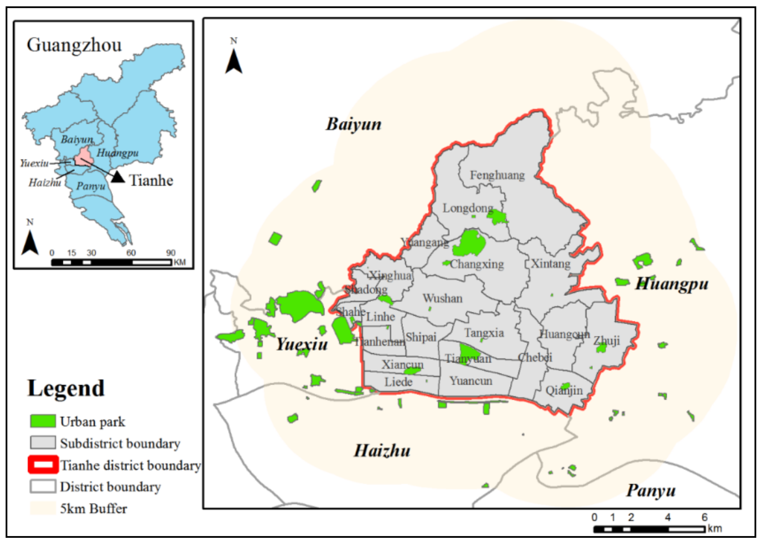
2.1. Study Area

This study was conducted in Tianhe District, located in the middle of Guangzhou (Figure 1). Tianhe District has a total terrestrial area of 137.38 km², which contains 21 subdistricts (called “jiedao”). According to the 2021 Seventh National Population Census, the current resident population of Tianhe District is 2,241,826. The transportation resources in the district are concentrated, with a multilevel urban transportation system that includes metro, bus rapid transit system, and urban ring expressway. Tianhe District is not only the most economically developed district in Guangzhou, but it also focuses on the transformation of green spaces to achieve the goal of “city in a park”.

The maximum service radius of municipal parks is 5 km (Guangzhou Greenland System Planning (2020–2035)) and related research shows that the average travel distance for metropolis residents, such as Beijing and Shanghai, is about 5–8 km [35]. Therefore, to mitigate the edge effect, we expanded our study area to a 5 km buffer zone around Tianhe District (Figure 1). The parks and population within the buffer zone were involved in the accessibility calculation, but only the results inside Tianhe District were researched and discussed.

2.2. Data Sources

2.2.1. Park Data

The list of parks and related data were obtained mainly from The Guangzhou Park List (as of the end of 2020) published by the Guangzhou Forestry and Landscape Bureau. A total of 64 parks were acquired, including 18 in Tianhe District and 46 in surrounding areas. The classification of parks was based on the classification standards of the Urban Green Space Classification Standard (CJJ/T85-2017) and the Special Plan for Guangzhou Park Construction and Protection (Draft) (2017–2035). There are 11 comprehensive parks, 17 theme parks, 25 community parks, and 11 pocket parks. The size of parks ranges from 0.49 ha to 300 ha, with an average of 19.13 ha. The park polygon layer data were mainly derived from the Open Street Map, Baidu area of interest (AOI) park data and were then compared and corrected with the online map. The smallest park in the OSM data is 23.2 square meters with a spatial resolution of about 5 m. In addition, the smallest park in the AOI data is 330 square meters with a spatial resolution of about 18 m. The geographic coordinate system was WGS1984 and the projection method was Universal Transverse Mercator (UTM). The actual entrance coordinates of the large parks were obtained through the Amap coordinate picker (https://lbs.amap.com/, accessed on 1 March 2022), with the centroids of the small parks (area ≤ 1 hm²) used as the entrance locations. Finally, the park polygon data and entrance data were transformed into the same coordinate system (WGS1984, UTM projection) and adjusted in corresponding spatial locations.

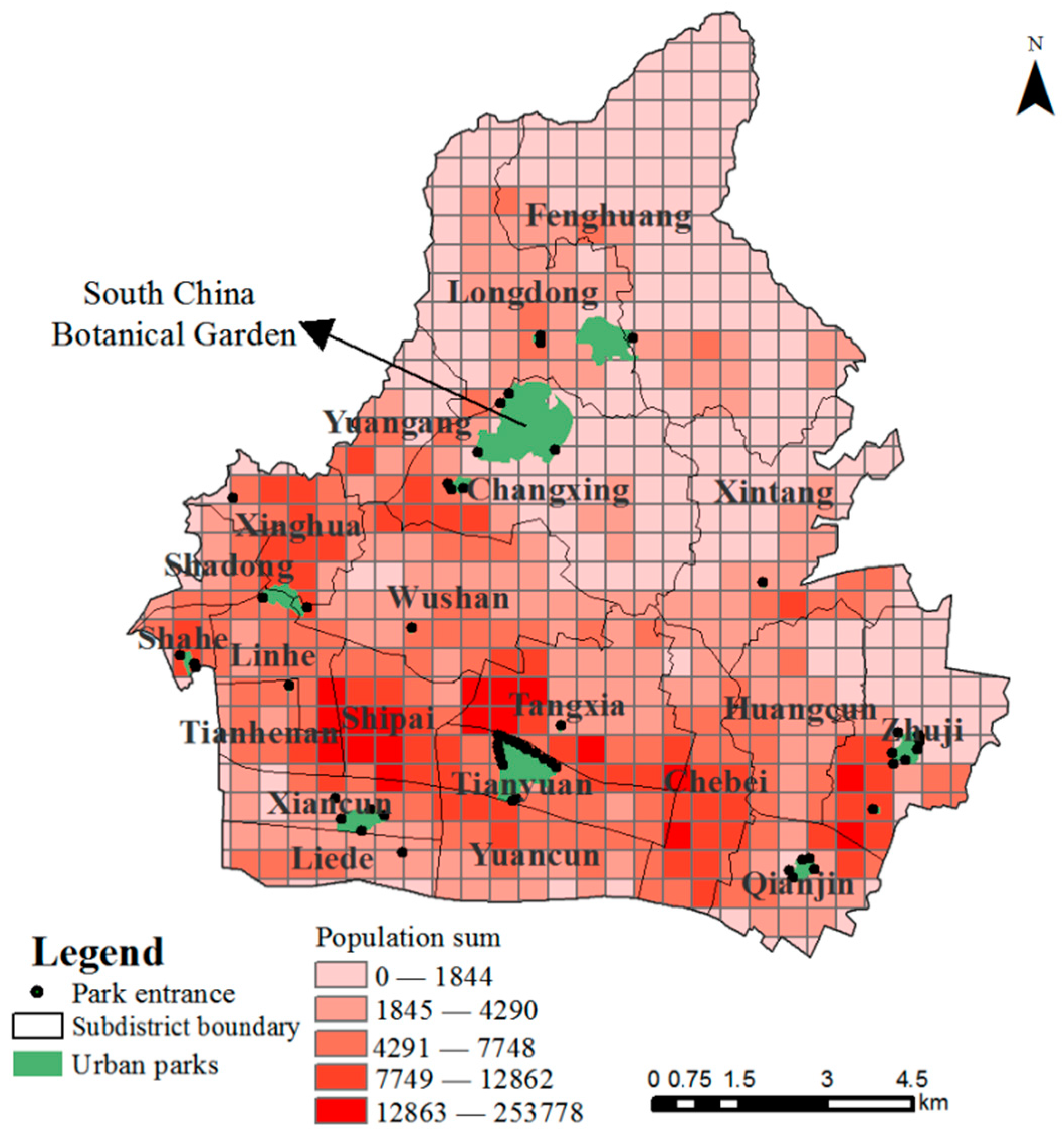
2.2.2. Population Data

To reduce the influence of spatial scale on accessibility evaluation, we studied the demand population in a 500 m × 500 m grid unit. The population data were provided by the 2020 WorldPop raster population data with a 100 m resolution (https://www.worldpop.org/geodata/summary?id=24926, accessed on 1 March 2022) and the 2021 Seventh National Population Census in Guangzhou. First, the population raster data were modified at the subdistrict scale with the census data. The correction coefficient was obtained by dividing the total census population by the total population of WorldPop of the corresponding subdistrict. Since the correction coefficient is a float number, the final population data were rounded to the nearest integer. Then, 500 m × 500 m grids were built in this area by ArcGIS 10.2 fishnet tool and 612 grids in Tianhe District were acquired. The population raster data were converted to point data, with the population-weighted centroids of each grid obtained as the demand point location. The total raster populations within each grid were calculated as the demand population number. We selected 500 m as the resolution because the coverage rate of park service areas is calculated at 500 m in the Special Plan for Guangzhou Park Construction and Protection (Draft) (2017–2035). In addition, the planned scale of the 5 min living circle is about 600 m × 600 m. Given the above two points, we used 500 m as the resolution, which is consistent with the planning scale and more convenient for practical management [36].

2.2.3. Travel Time Data

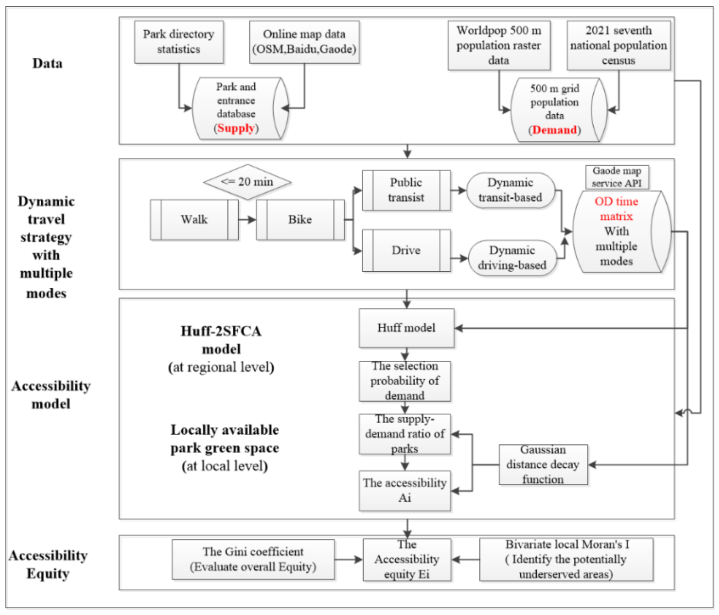
Real travel time data were obtained using the route planning web service API of Gaode map (https://lbs.amap.com/api/webservice/guide/api/direction, accessed on 1 March 2022). Transport modes included walking, biking, public transit, and driving. First, by setting a grid population-weighted centroid as the origin (O) and all entrances of a park as the destination (D), the travel time for each OD pair was calculated using Python. The shortest time was then selected as the travel time for this grid to reach the park. Through cyclic calculation, the travel time from each grid to all parks was finally obtained. To avoid commuting congestion, we selected 10:30–16:00 on weekends as the data collection time.

2.3. Methodology

Figure 2 represents the framework proposed in this study. A H2SFCA model based on supply and demand was used to quantify the accessibility levels. Three key elements of the H2SFCA model were population data (demand), urban park locations, and area data (supply), as well as the travel time between demand and supply.

2.3.1. Accessibility Model: An H2SFCA Model

To estimate the selection probability of demand, we initially used the Huff-based competitive model, as shown as follows:

$$Pro{b}_{ij}=\frac{S_{j }\times W_{ij}}{{{\displaystyle \sum }}_{i\in \left\{t_{ij}\le t_0\right\}}{S}_j\times W_{ij}},$$

(1)

$$W_{ij}=\left\{\begin{array}{l}\hspace{1em}{t}_{ij}^{-\beta },\hspace{1em}\hspace{1em}if t_{ij}\le t_0\\ \hspace{1em} 0, if t_{ij}>t_0\end{array}\right. ,$$

(2)

where Prob_ij is the probability of residents in grid i traveling to park j and S_j is the service capacity of park j, which is represented by the park area here. β is the distance decay coefficient, which is typically set from 1.5 to 2 [34]. Given that the distance weight is higher than the area weight of the park when residents choose the park, β in this paper is set to 2.

By combining the Huff model and the 2SFCA model (H2SFCA), we then calculated a spatial accessibility score for each grid in Tianhe District. The implementation process of H2SFCA is divided into two steps.

Step 1: Calculate the supply–demand ratio.

For each supply park point j, we searched for all demand points k that were within the time threshold t₀. Next, the populations of demand point k were weighted according to the Huff model and Gaussian function and were summed to obtain all the potential demands of park supply point j [34]. Finally, the area of supply point j divided by the demand population is the supply–demand ratio R_j in Equation (3).

$$R_j=\frac{S_j}{{{\displaystyle \sum }}_{k\in \left\{t_{kj}\le t_0\right\}}Pro{b}_{kj}\times G\left(t_{kj},t_0\right)\times P_k},$$

(3)

where Sj is the supply of park j, which can be expressed by the area size of the park; t_kj is the travel time from demand point k to the park j; Prob_kj is the probability of residents in grid k choosing park j; P_k is the population of demand point k; and G(t_kj, t₀) is a Gaussian distance decay function, as shown in Equation (4).

$$G\left(t_{kj},t_0\right)=\left\{\begin{array}{l}\frac{e^{-\frac{1}{2}\times \left(\frac{t_{kj}}{t_0}\right)2}-e^{-}{}^{\frac{1}{2}}}{1-e^{-}{}^{\frac{1}{2}}}, if t_{kj}\le t_0\\ 0, if t_{kj}>t_0\end{array}\right.$$

(4)

Step 2: Calculate the accessibility.

For each demand point i, we searched for all supply park points j that were within the time threshold t₀. We then calculated the accessibility of point i by summing the supply–demand ratio R_j. The accessibility value A_i (Equation (5)) could be interpreted as the per capita PGS area [34].

$$A_i={\displaystyle \sum }_{i\in \left\{t_{ij}\le t_0\right\}}Pro{b}_{ij}\times G\left(t_{ij},t_0\right)\times R_j,$$

(5)

where R_j is the supply–demand ratio of park supply point j within the time threshold t₀ and t_ij is the travel time from supply point j to demand point i. Prob_ij and G have the same meaning as above.

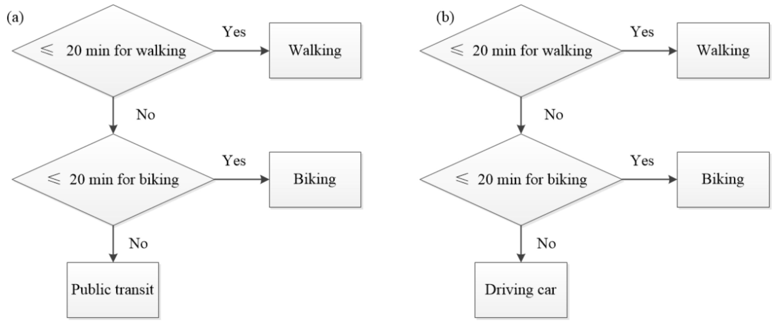
2.3.2. Dynamic Travel Modes

People can flexibly choose how to travel to parks based on travel time, transportation facilities, and their socioeconomic status. As a result, estimates of park accessibility using a fixed travel mode would be biased. For example, residents near the park would prefer walking or cycling, but residents far away would choose public transport or driving. In China, private cars and public transport are the main ways for urban residents to travel long distances [37]. Thus, we created a multimodal travel strategy by combining walking, biking, public transport, and driving to measure park accessibility (Figure 3). This strategy assumes that people use public transit or driving cars for long-distance travel, whereas prefer walking or cycling for short distances. If the travel time is less than 20 min, then walking is selected first, followed by biking; if the travel time is more than 20 min, then public transit or driving is selected. This strategy includes two scenarios, as shown in Figure 2. Scenario (a) is a dynamic transit-based mode and scenario (b) is a dynamic driving-based mode, which are suitable for different people. Here, we set a threshold of 20 min because people generally tolerate walking and biking for less than 20 min [23,24,37]. A previous study suggested that walking or biking for 15–25 min per day is better for people’s health [38].

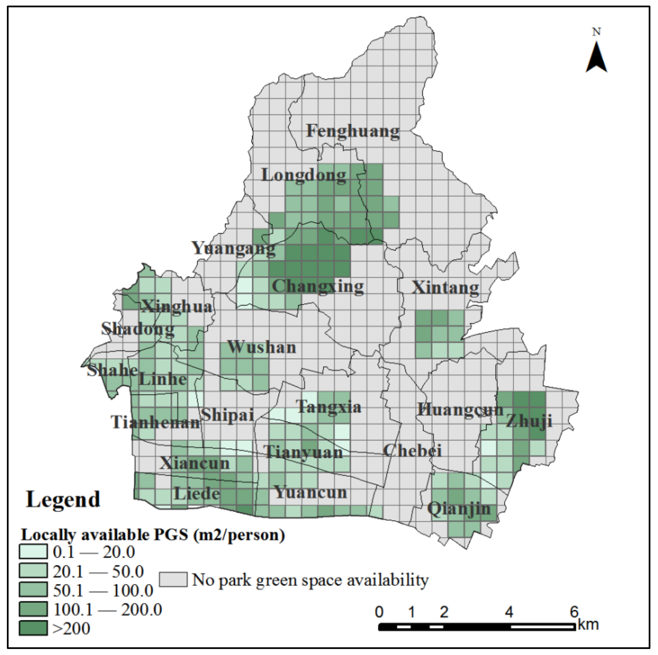
2.3.3. Locally Available Park Green Space

Locally available park green space means per capita area of PGS (m²/person) within a certain range of residents’ living, which reflects the availability and accessibility of PGS at a local scale [39,40]. It is an important indicator of PGS provision [41]. According to the requirements of the government for citizens to walk no more than 500 m to park green space (PGS), the acceptable walking distance is set to 500 m in this research. First, we make a buffer zone of 500 m away from the park green space, and intersect with the population grid to calculate the green space buffer zone area of each grid. The total population of each grid in the buffer zone is then counted. Finally, by dividing the PGS area by the population sum, per capita area of available PGS can be calculated.

2.3.4. Gini Coefficient and Bivariate Local Moran’s I index

The Gini coefficient measures park accessibility distribution across a population and ranges from 0 (perfectly equal) to 1 (perfectly unequal) [42]. It is calculated as follows [43]:

$$G_m=1-{\displaystyle \sum }_{k=1}^n\left(B_k-B_{k-1}\right)\left(C_k+C_{k-1}\right),$$

(6)

where G is the Gini index, B_k is the cumulative proportion of population, C_k is the cumulative proportion of accessibility, and n is the number of grids.

The Lorenz curve graphically represents the accessibility concentration at each percentile of the population. The greater the degree of curvature of the Lorenz curve, the more unfair the spatial distribution of park accessibility will be. The Gini coefficient measures the overall equity, whereas the bivariate local Moran’s I index measures the spatial clustering in the association between park supply and people demand. The bivariate local Moran’s I index and cluster map were obtained using GeoDa software. The bivariate Moran’s I value was used to calculate the spatial autocorrelation between the accessibility value of PGS and population density.

3. Results

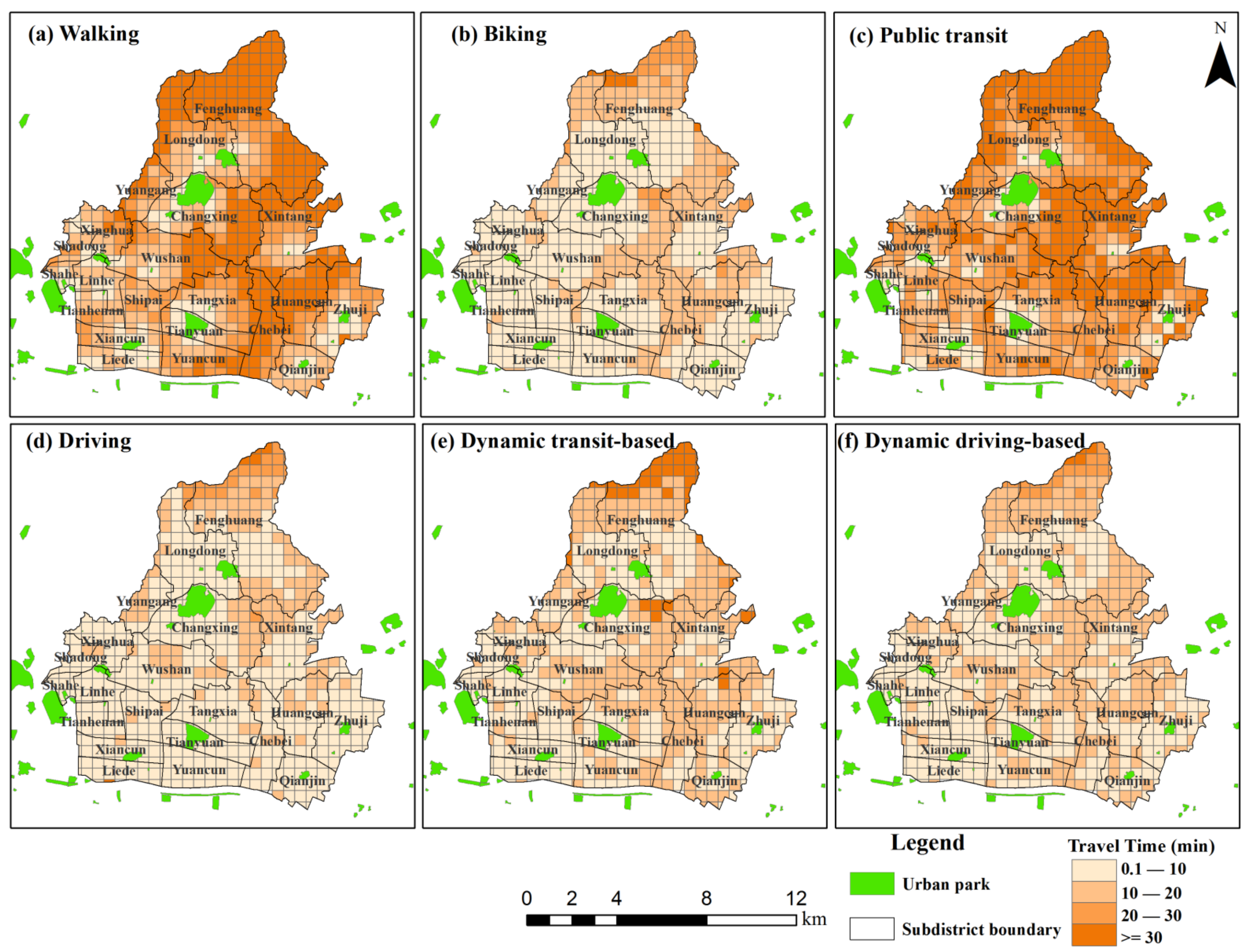
3.1. Analysis of Travel Time for Different Modes

Figure 4 shows the population and park distributions in Tianhe District. The population is mainly concentrated in the southern and western areas. However, the distribution of parks shows a discrete distribution trend, with the northern and eastern fringe areas less distributed. Through Gaode map path planning, we calculated the time it takes for grid points to reach the nearest park for four travel modes: walking, biking, transit, and driving. According to the framework (see Figure 2), we then calculated the travel time for two dynamic modes. The results show that driving and biking have a lower mean travel time, followed by dynamic transit- and driving-based modes, whereas public transit and walking have an average travel time that is more than three times longer than that of driving and biking (see

Table 1. Statistical analysis of travel time for different modes.

Travel Mode	Max	Min	Mean	SD	N10 min	N20 min	N30 min
Walking	148.75	0.43	28.94	21.55	88 (14.38%)	246 (40.20%)	381 (62.25%)
Biking	44.75	0.02	9.52	6.69	379 (61.93%)	566 (92.48%)	602 (98.37%)
Public transit	122.50	0.43	28.61	18.57	72 (11.76%)	179 (29.25%)	385 (62.91%)
Driving	41.37	0.12	9.06	5.32	441 (72.06%)	582 (95.10%)	607 (99.18%)
Dynamic transit-based	122.50	0.43	14.95	18.69	299 (48.86%)	566 (92.48%)	567 (92.65%)
Dynamic driving-based	34.18	0.43	10.33	4.41	329 (53.76%)	586 (95.75%)	608 (99.35%)

Max is the maximum time to reach the nearest park; Min is the minimum time to reach the nearest park; Mean is the average time to reach the nearest park; SD is the standard deviation of the mean time to the nearest park; N10 min, N20 min, and N30 min represent the number of grids reaching the nearest park within 10, 20, and 30 min, respectively^.

).

The number of grids reaching the nearest park in different time thresholds for multiple travel modes was also counted. More than 60% of the grids can reach the nearest park within 30 min with six travel modes. However, for walking and public transit, the number of grids that can reach the nearest park is significantly less than that by other travel modes. For example, more than 90% of the grids can reach the nearest park within 20 min by biking, driving, and dynamic modes, whereas less than 50% of the grids can reach the nearest park within the same time by walking and public transit.

To explore the spatial disparity of travel time in Tianhe District, we also mapped the average travel time from the grid to the entrance of the nearest parks by different travel modes (see Figure 5). Travel time is related to the distribution density of the park and the travel speed. The results show that people living in the midwest region are likely to have a shorter travel time because more parks are concentrated there. The spatial patterns of walking and public transit modes are similar, where only the grids near parks or adjacent transit lines have short travel times. The dynamic modes have a more discrete spatial distribution of travel time because of the collection of multiple modes. Moreover, the travel time to the nearest park in Chebei and Huangcun Subdistrict by driving is considerably shorter than that by biking. On the contrary, in parts of Wushan Subdistrict, biking is more convenient than driving to the nearest park. Thus, people’s choice of transportation mode will affect the corresponding route and time. When calculating accessibility, the influences of travel modes should be considered.

3.2. Accessibility Analysis for Different Modes

Because park green space has different functions, residents will choose the corresponding park green space to carry out leisure activities. If there are pocket parks available locally, most residents will choose to walk there for leisure. However, if they want to take children for recreation or picnic, they will generally choose a nearby park with a larger area—such as a children’s park or a comprehensive park—that they can access by different travel modes. Therefore, the accessibility of park green space can be measured from two aspects: one is the accessibility at regional level and the other is the availability at local level.

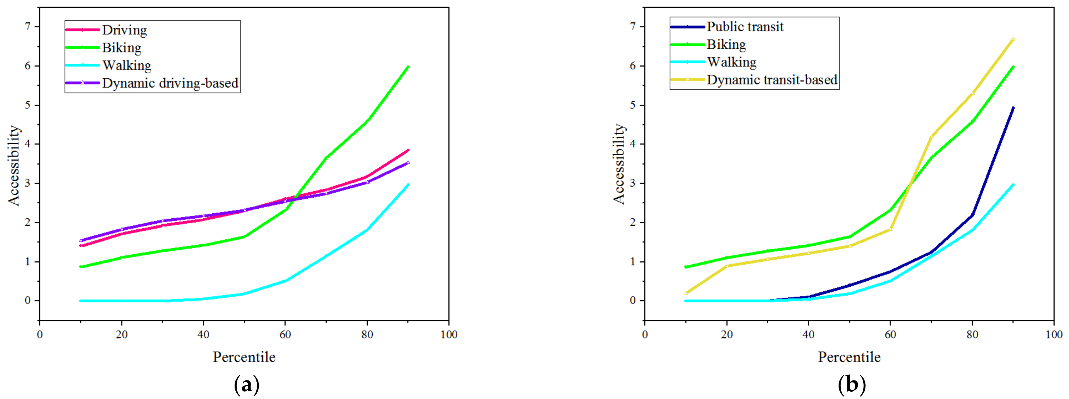
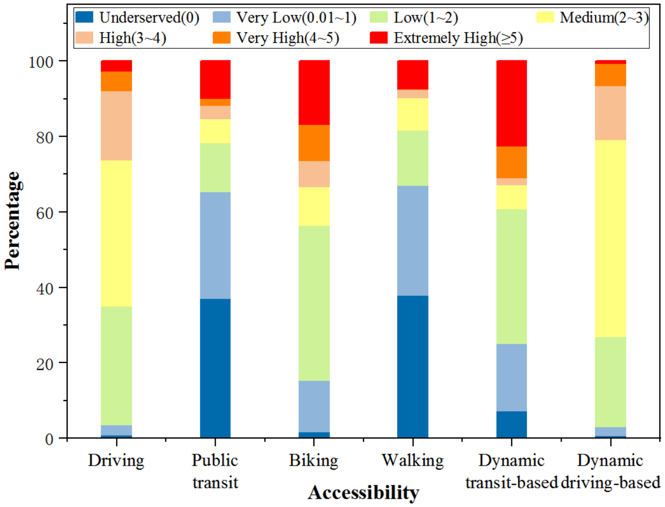
3.2.1. Numerical Statistical Analysis of Accessibility

According to the statistics in Table 1, the maximum average travel time from the grid to the nearest PGS is about 30 min for multiple travel modes. Here, the time threshold in the accessibility calculation was also set as 30 min, which was used to characterize the average travel level arriving at PGS at regional level [26].

From a statistical perspective, the maximum, mean, and standard deviation of the accessibility value for the dynamic driving-based mode are all lower than those for associated single modes, and the underserved number of grids for the dynamic driving-based mode is also reduced (see

Table 2. Dynamic driving-based and related single-modal accessibility statistics.

Travel Mode	Max	Min	Mean	SD	Underserved Grid Number
Walking	67.45	0.00	2.93	10.20	293
Biking	9.84	0.00	2.64	2.55	24
Driving	7.58	0.00	2.49	1.43	11
Dynamic driving-based	7.56	0.00	2.46	1.24	8

Max is the maximum accessibility; Min is the minimum accessibility; Mean is the average accessibility; SD is the standard deviation of accessibility values. The underserved number of grids is defined as the number of grids with an accessibility value equal to 0.

). The maximum, mean, and standard deviation, as well as the underserved number of grids for dynamic transit-based accessibility, are lower than those for transit and walking, but higher than those for the biking mode (see

Table 3. Dynamic transit-based and related single-modal accessibility statistics.

Travel Mode	Max	Min	Mean	D	Underserved Grid Number
Walking	67.45	0.00	2.93	10.20	293
Biking	9.84	0.00	2.64	2.55	24
Public transit	79.40	0.00	2.82	10.63	319
Dynamic transit-based	10.52	0.00	2.65	2.62	46

Max is the maximum accessibility; Min is the minimum accessibility; Mean is the average accessibility; SD is the standard deviation of accessibility values. The underserved number of grids is defined as the number of grids with an accessibility value equal to 0.

). In addition, the maximum accessibility value by walking and transit modes are significantly higher than other modes. The parks’ serviceable population shrinks within the same time threshold due to the low speed of public transport and walking. Thus, there exist significantly high supply–demand ratios in large-area parks such as the South China Botanical Garden, while the accessibility value of the adjacent grids is also significantly high. On the contrary, the accesses of driving, biking, and dynamic modes are longer; thus, the supply–demand ratio of the same park is relatively less. In addition, residents can choose more parks, and the region with large-area parks can compensate for the small-area parks in the surrounding area, which will weaken the effect of the difference in the supply–demand ratio of parks; hence, the accessibility value is smoother.

The average value is affected by some significantly high accessibility values and cannot represent the overall distribution of accessibility indicators of each mode. Therefore, we also analyzed and compared the accessibility values at different quantiles (see Figure 6). (1) We compared the dynamic driving-based accessibility with the three related single travel modes. The results show that in the 10–90% percentile, the accessibility value by the dynamic driving-based mode is higher than that by walking, which is similar to that by driving. When the accessibility value is within the 60th percentile, the accessibility value for the dynamic driving-based mode is higher than that for the biking mode; however, when the accessibility value is between the 60th and 90th percentiles, the dynamic driving-based accessibility value is lower than that of the biking mode. (2) We also compared the dynamic transit-based accessibility with the related single travel modes. The results show that in the 10th–90th percentile, the accessibility value of the dynamic transit-based mode is higher than that of the public transit and walking modes. When the accessibility value is within the 60th percentile, the accessibility value of the dynamic transit-based mode is lower than that of the biking mode, but when the accessibility value is between the 60th and 90th percentiles, the dynamic transit-based accessibility value is higher than that of the biking mode. Generally, the supply–demand ratio of the park and the travel time influence the accessibility value, and the accessibility comparison relationship under different quantiles is more complicated.

To further investigate the relationship between dynamic and single travel modes, we used the Pearson coefficient to analyze their correlation. As shown in

Table 4. Pearson correlation coefficient between dynamic mode and related single-mode accessibility.

Travel Mode	Walking	Biking	Public Transit	Driving
Dynamic transit-based	0.465 **	0.941 **	0.455 **	/
Dynamic driving-based	0.573 **	0.712 **	/	0.746 **

** Significantly correlated at the 0.01 level (two-sided).

, accessibility values for dynamic modes are positively correlated with that of single modes. Specifically, the dynamic transit-based mode is mostly correlated to biking, while the dynamic driving-based mode is mostly correlated to driving and biking. This finding indicates that most grids are suitable for biking and driving modes to reach the park, with the calculation process of dynamic mode accessibility tending to obtain a larger search range.

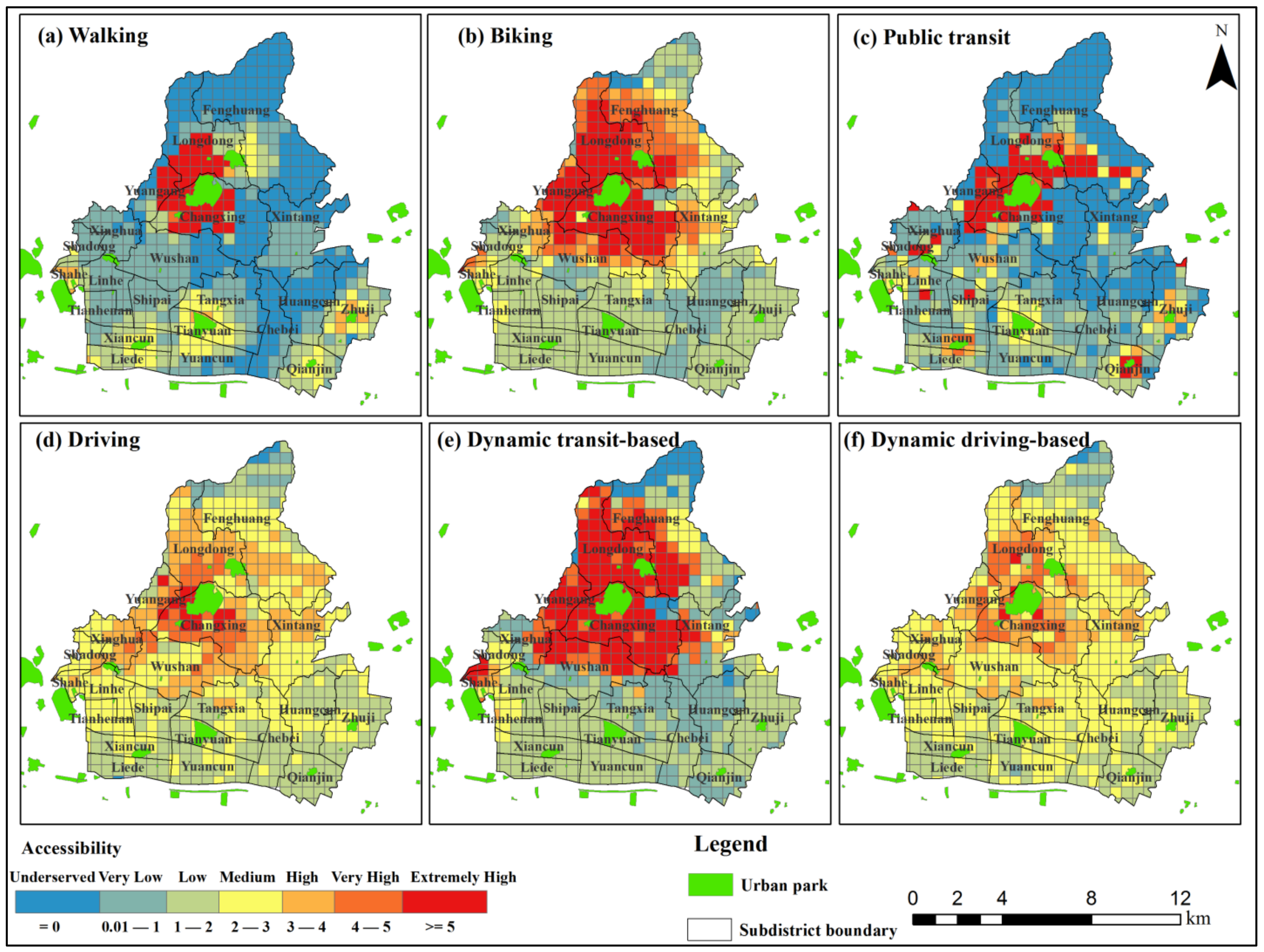
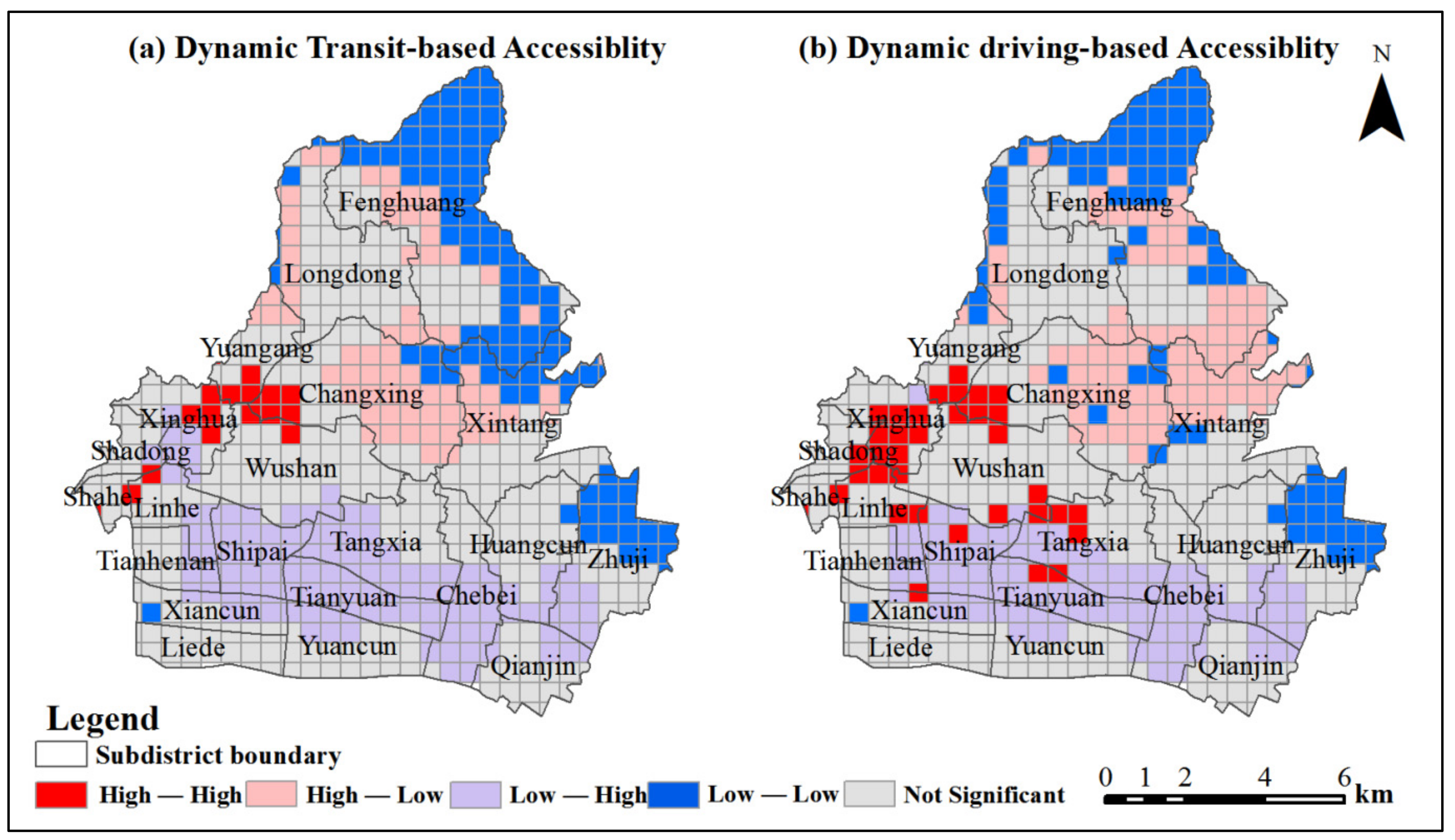
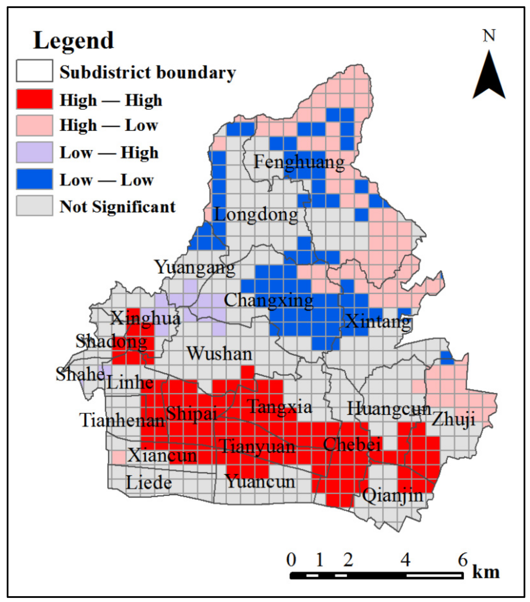
3.2.2. Spatial Distribution Analysis of Accessibility

The accessibility value refers to the per capita availability of PGS by a particular mode of travel. Figure 7 shows the accessibility value map of different travel modes in Tianhe District at regional level. The accessibility value ranges were divided into seven groups and were distinguished by different colors. Redder colors indicate higher accessibility, whereas bluer colors indicate lower accessibility. The results show that the accessibility distribution varies by travel mode. Grids with high accessibility values are located near larger parks and with less dense surrounding populations, whereas grids with low accessibility values are further away from parks.

For single modes, the areas with low accessibility (value < 1) by walking and public transit are significantly larger than those by biking and driving, which indicates that most residents cannot access parks by walking or public transit. In addition, the accessibility distribution is closely related to the traffic conditions. The accessibility pattern for the public transit mode is mainly affected by the subway lines and stations; the biking mode is mainly affected by impenetrable highways, rivers, and other terrain obstacles; and the driving mode is mainly affected by the road density and traffic condition.

To further explore the differences in the accessibility distribution between dynamic and single travel modes, we compared the spatial extent percentage of accessibility at various levels (see Figure 8). For the dynamic transit-based mode, the overall level of accessibility is better than that for walking and public transit. The number of grids with extremely low (≤1) and extremely high (>5) accessibility values for the dynamic transit-based mode exceeds that for biking, whereas the number of grids with medium and high accessibility values (1–5) is less than that for biking. A possible reason is that the biking mode overestimates the residents’ access with a travel time greater than 20 min; thus, the accessibility value increases. Conversely, for the dynamic driving-based mode, the overall level of accessibility is better than that for the single walking mode, as the grids with medium and high values are not limited to the periphery of the park. In comparison with driving and biking, the low- and high-value accessibility extent of the dynamic driving-based mode is smaller, whereas the intermediate accessibility value extent of the dynamic driving mode is larger. For example, a comparison of the dynamic driving-based mode and the single driving mode shows that the high-value accessibility extent (≥3) near the South China Botanical Garden decreases, whereas the medium value accessibility extent (2–3) in the southern area increases. Generally, the dynamic driving-based mode reduces the estimation of extreme values. Thus, the overall accessibility values tend to be more in the middle range, with the spatial disparity between them considerably smaller.

On the other hand, residents will also tend to go to the surrounding parks and green spaces in their daily lives. Therefore, we further analyze the park green space availability at a local level. The results show that the PGS availability pattern is similar to the accessibility by walking (see Figure 9). The number of grids without PGS availability is 408 and the standard deviation is 84.88. The underserved grid number is higher than that in accessibility by walking. Overall, the availability of PGS is related to the location, size of PGS, and local population density.

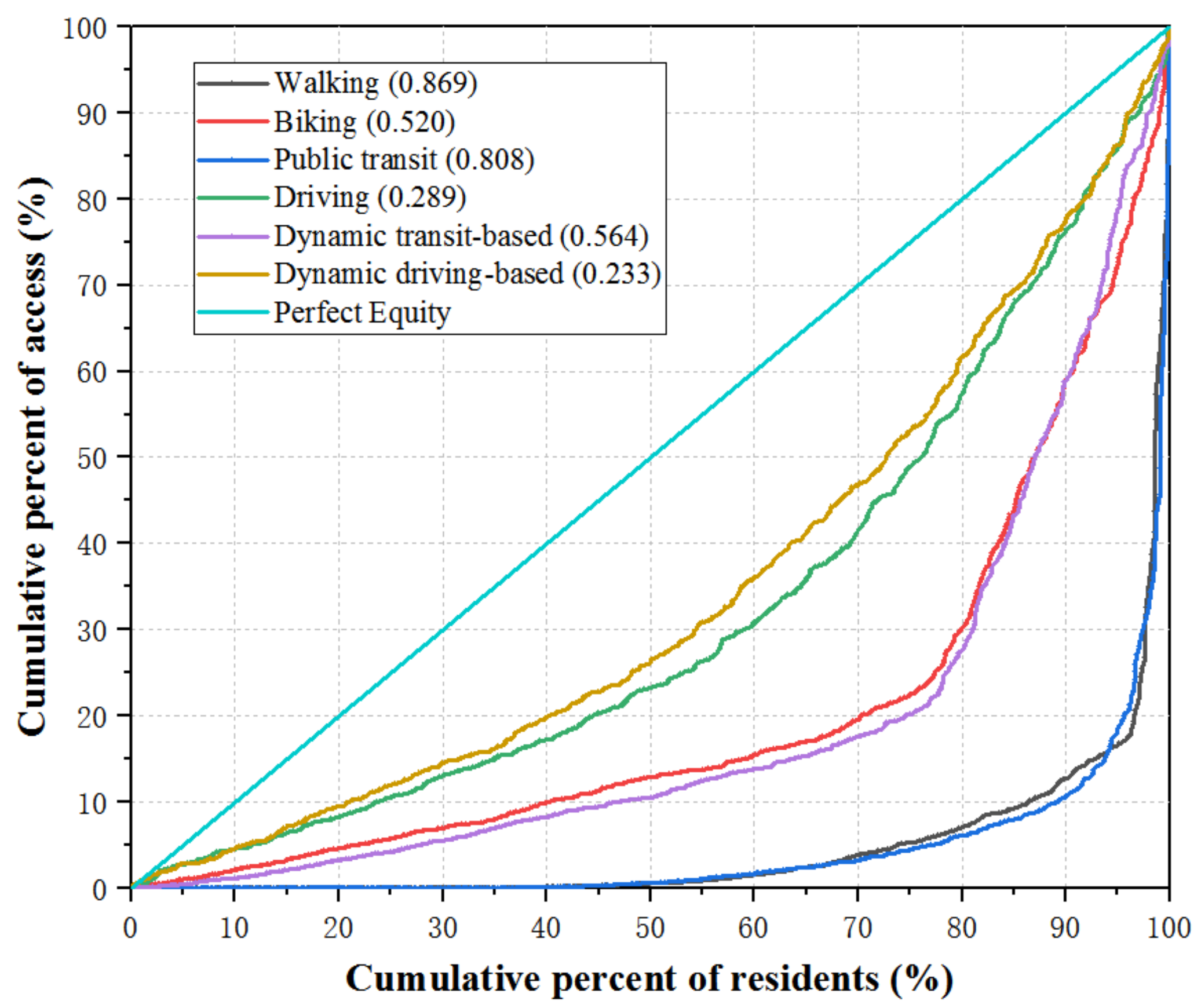
3.3. Accessibility Equity Analysis for Different Modes

3.3.1. Gini Coefficient Statistical Analysis

The Lorenz curve [42] graphically represents the distribution of green space resources among the resident population. The value of the Gini coefficient ranges from 0 to 1. The lower the Gini coefficient, the more equal the residents’ access to public green space resources will be, with 1 being completely unequal. We calculated six Lorenz curves and Gini coefficients to compare the equity of park accessibility for different travel modes (see Figure 10). The results show that there exist differences in the park accessibility equity under different travel modes. Park accessibility equity is best in the dynamic driving-based mode, followed by driving and biking, dynamic transit-based mode, and finally public transit and walking modes. The accessibility equity for the dynamic driving-based mode is improved compared to the single driving mode, as indicated by the Gini coefficient value decreasing from 0.289 to 0.233. Similarly, the accessibility equity in the dynamic transit-based mode is also improved compared to the single transit mode, with the Gini coefficient decreasing from 0.808 to 0.564. This result suggests that park accessibility is more equitable by dynamic modes. Using a single model may underestimate the accessibility equity of parks.

3.3.2. Correlation Analysis of Accessibility Distribution and Population Density

To identify the spatial differences in equity for dynamic transportation modes, we conducted a spatial correlation analysis. Park accessibility can reflect the supply and demand relationship between the population and PGS. From the perspective of supply and demand balance, areas with high population density also have high population activity; thus, the accessibility of PGS has a greater influence there. Therefore, to better understand the matching relationship between the supply of urban green space and the demand of the residential population, we conducted a correlation analysis between the accessibility distribution and population density.

As shown in

Table 5. Bivariate Moran’s I value for dynamic modes.

Bivariate Index	Moran’ I	Z-Value	p-Value
Dynamic driving-based mode and population	−0.036 *	−2.2613	0.014
Dynamic transit-based mode and population	−0.136 **	−8.7418	0.001
The gap between two dynamic modes and population	0.157 **	10.1822	0.001

** Significantly correlated at the 0.01 level (two-sided), * Significantly correlated at the 0.05 level (two-sided).

, the two-variable global Moran’s I value is negative in the two dynamic traffic modes, which are −0.036 and −0.136, and have passed the 5% significance level test. This result shows that a negative spatial correlation exists between the accessibility value and population density for dynamic transit- and driving-based modes, indicating that park accessibility in Tianhe District is not coordinated with the spatial distribution of population. Further bivariate local Moran’s I was used to classify and analyze the clustering situation, which was divided into high accessibility and high population density (High-High), low accessibility and low population density (Low-Low), low accessibility and high population density (Low-High), and high accessibility and low population density (High-Low) (see Figure 11). The results show that for the two dynamic models, the Low-High areas account for a large proportion. Thus, the park service capacity of these areas is lower than the population demand. The Low-High areas mainly distribute in Shipai, Tianyuan, Chebei, and Tangxia Subdistricts, and are the key areas to be improved in the next planning.

Next, to analyze the influence of the accessibility gap for two dynamic modes, spatial correlation analysis was performed between the accessibility gap and population density. The results show that the accessibility gap between dynamic transit- and driving-based modes is positively correlated with population density (see Table 5). High-High cluster areas are located in the southern part of Tianhe District, mainly including Shipai, Tianyuan, and parts of Tangxia and Chebei Subdistricts (see Figure 12). Therefore, in the context of advocating sustainable transport, these High-High cluster areas should be prioritized to reduce the inequality of access to park services by public and private transportation.

4. Discussion

4.1. Advantage

Most early accessibility models have used a single travel tool to measure park accessibility because such models assume that all residents use the same travel mode to access parks [27,30,44]. However, people in different locations may choose various travel modes to enter the park. Some studies have indicated that the nearby green space supports human health, and distance is very important [45,46]. For example, residents near the park will prefer walking or biking, but residents far away from the park will like public transport or driving. According to the local traffic conditions, this study comprehensively considered non-motorized transportation and motorized transportation initially and then designed “walking or biking or public transit” and “walking or biking or driving cars” as two dynamic travel scenarios. In view of multiple travel modes and different park selection probabilities to improve the 2SFCA method, dynamic transit- and driving-based accessibility models were proposed. Finally, in the context of advocating a policy of prioritizing the development of public transport, areas for improvement were identified through supply and demand analysis. In comparison with previous studies, our improved model has the following advantages: (1) A 500 m × 500 m grid was used as the basic analysis unit. Most previous studies have used subdistricts or communities as research units [24,33]. Larger administrative boundaries may cause deviation of travel time estimation. Small-scale analysis is more accurate in time calculation and helpful in discovering spatial variability. (2) Map service API was used to estimate travel time. Given that online maps consider transit times and real-time traffic conditions, they are more reliable than road network analysis by assigning speeds. (3) According to the travel time between the demand and supply points, the travel mode for a specific demand point was dynamically selected. Meanwhile, in view of the residents’ choice probabilities of parks with different service capabilities, a dynamic H2SFCA model was constructed. This model can provide some improvements to the accessibility measures of a single travel mode. The research outcomes also enrich the study of spatial mismatch between urban park green resources and population distribution for public transit and driving in two scenarios.

4.2. Interpretation and Application

In this paper, we initially calculated the average travel time from the grid to the nearest park for multiple travel modes using the Gaode map routing function. These modes included four single modes of walking, biking, public transit, and driving, and a combination of dynamic transit- and driving-based modes. The results show that driving and biking modes have more significant spatiotemporal compression effects than public transit and walking modes. This finding is similar to that of a previous study [18,26]. Bicycle travel is more convenient than public transit because of the density of public transport stops and transfer times [33]. The travel time of the two dynamic modes is greater than that of biking and driving and less than that of public transit and walking. The main reason is that the dynamic modes combine multiple travel modes, so their average speed is between that of the fast and slow modes.

The statistical results and spatial disparity of park accessibility for dynamic and single travel modes were then compared. Statistical results show large differences in accessibility values by walking, biking, public transit, and driving, suggesting that a single-mode model may not be able to reliably assess park accessibility [27,29,30]. Previous studies have shown that the mean and standard deviation of accessibility by multiple modes are slightly lower than that by single-mode methods [24]. However, our results for the dynamic public transit mode are not entirely consistent, which may be due to our study considering the public transit mode (such as bus and metro) and set a smaller spatial scale unit. Public transit accessibility is more dependent on route and station distribution [28], so the comparison relationship is more complicated. In addition, a finer study scale may also make it easier to show data differences. Accessibility results need to be interpreted based on travel mode and estimated time thresholds. Disparities exist in accessibility at the local and regional levels, especially for different modes of transportation. The smaller the access area is, the more uneven the allocation of park resources will be [39]. Although there is park green space within a certain distance, an excessively high population density often leads to little park green space available per capita.

Comparison of the accessibility distribution pattern for different travel modes shows that the high-value accessibility extent of the dynamic transit-based mode is larger than that of the single transit mode. For the single public transit mode, only the areas around the park or near the main bus line have a higher accessibility value, whereas the remaining areas have a relatively lower accessibility value. However, the dynamic transit-based mode includes walking, biking, and public transit. People can more easily access parks by dynamic transit than by a single transit mode. Thus, the number of underserved areas is significantly reduced, and the range of medium and high accessibility values is significantly increased. Conversely, the medium accessibility value range by the dynamic driving-based mode is larger than that by single driving. For the single driving mode, high-value areas are mainly distributed near the South China Botanical Garden (see Figure 4). The density of vehicle roads there is low and suitable for biking or walking. More people can reach the park by the dynamic driving-based mode; thus, the population served by the park increases, resulting in a significant decrease in the supply–demand ratio. Meanwhile, the number of accessible parks does not increase significantly, so the corresponding high accessibility value decreases. In general, the accessibility value is mainly determined by the supply–demand ratio of parks and travel time. Given that dynamic modes integrate various travel modes, they can select the appropriate traffic tool according to the location environment and objectively estimate the access range and the supply–demand ratio of the park. To a certain extent, accessibility results are more realistic and can reduce estimation errors caused by a single travel mode.

Further results show that the park accessibility equity of dynamic transit- and driving-based modes is considerably improved compared to single public transit and driving, respectively, which indicates that park accessibility by the mixed mode has better spatial equity [26]. This finding provides information and support for advocating that residents choose multiple travel modes, especially non-motorized transportation. Managers can encourage residents to take different travel tools according to local conditions, such as walking or biking or using public transit for short-distance travel and promoting green travel behavior. Notably, a large gap exists between the accessibility of parks for dynamic transit- and driving-based modes in the southern surrounding areas, which is closely related to the limited public transport conditions and the sparse distribution of parks. Therefore, in the context of advocating green travel, we need to focus on park service equality in the above areas. A feasible method is to coordinate the spatial layout of public transport and parks in these areas [47,48], especially improving bike lane coverage, increasing and optimizing bus routes connecting the parks, and scientifically selecting park sites.

Through rational planning of travel modes in different urban spaces, the equity of residents’ enjoyment of park resources will be improved. The results show that the accessibility distribution varies by travel mode. At the local level, walking is the most common mode of transportation, but its travel efficiency is lower than other travel modes. Those places with better PGS availability are located around large parks and have a small population [39,40]. Biking is faster than walking. The areas with better public transit accessibility are distributed along the subway and bus stations, but the support for urban marginal areas is weak. Cars are mainly affected by road conditions and have the widest range of accessibility within the same time limit, which can alleviate the current situation of poor accessibility in the marginal area to a certain extent. For example, in areas with dense parks in the central city, road conditions are often congested and the population density is high. Biking or walking is recommended. However, in areas with sparse parks on the edge of the city, road conditions are relatively good and the population density is small. Due to the limited walking distance, it is recommended to use driving or biking to expand the access range and increase the convenience of reaching the park. In addition, public transport can also be developed to provide more options for settlements far from parks. To a certain extent, the level of park accessibility can be improved by choosing the appropriate travel mode according to the local context. Furthermore, differences in the spatial allocation of park green space resources can be reduced.

The above analysis and empirical results show that the dynamic accessibility model can be used as a new attempt for measuring accessibility and character analysis and can also provide a comprehensive measure of public transport services for urban parks or other public utility services. In addition, because high-income people tend to travel by car and low-income people by public transport [41], using two dynamic models can further assist in evaluating an in-depth analysis of the equity of people with different incomes accessing parks.

4.3. Limitation

Some limitations are still present in this paper. First, when evaluating the service capacity of PGS, only the area of the park is computed, whereas the park types’ [49], internal facilities [50] and landscape environments [51] are not considered. The attitude of residents is also an important influencing factor. These factors all affect the attractiveness and accessibility of the park. It is necessary to comprehensively analyze the accessibility of park green space from different aspects. Second, residents have limited tolerance time for different types of parks and travel modes [52]; thus, further refinement of the time threshold is required for future research [53]. Third, this paper focuses on all groups in the study area. The accessibility equity of different groups or specific groups is still a direction worthy of further in-depth study [54]. In addition, the impact of parks on environmental health, especially the impact of a park’s soil on the ecosystem service, is also an important aspect that needs attention [55,56].

5. Conclusions

The main objective of this study was to evaluate accessibility level for dynamic travel modes. As residents choose travel modes based on the distance or road condition to the target park, we fully considered multiple travel modes and dynamically selected the appropriate transport mode for a specific location. Moreover, public transit and driving cars are common means of long-distance travel, whereas walking and biking are more suitable for short-distance travel. Thus, in view of the above four travel modes and different park selection probabilities to improve the 2SFCA method, the dynamic transit- and driving-based accessibility models at the grid scale were proposed.

The results suggest that reaching the nearest park is faster by bike and car, with the dynamic traffic mode being slower. In addition, the accessibility statistical characteristic and spatial pattern were analyzed using the H2SFCA model in different travel modes. The PGS availability pattern at the local level is more uneven than the distribution of accessibility at the regional level. The evaluation results of park accessibility are largely affected by the residents’ travel modes. The accessibility for the single travel mode is more likely to overestimate or underestimate some grids or exhibit a significantly low or high value. This bias is especially pronounced for grids in remote areas or near parks. Finally, accessibility equity of different modes was estimated by a Gini coefficient and cluster map. The results suggest that park accessibility equity is best for the dynamic driving-based mode, followed by driving and biking, the dynamic transit-based mode, and finally the public transit and walking mode. This finding indicates that using a single model may underestimate the accessibility equity of parks, and residents can select suitable travel tools to obtain more equitable park services. Furthermore, there is a significant difference between dynamic driving-based accessibility and dynamic transit-based accessibility in the south of Tianhe District. Given the objective of promoting public transport travel in future planning, attention should focus on the coordination of public transport facilities services and park distributions in the above areas.

The dynamic H2SFCA method proposed in this study provides improved technical methods for measuring park accessibility in areas with diverse travel modes. Two scenarios, dynamic transit- and driving-based modes, were designed to help compare accessibility disparity in a more realistic way. This method can be used as a measure of public transport services in parks on a refined spatial scale and can also be further combined with detailed population data to evaluate the fairness of park services for different income groups. This study is of great significance for coordinating traffic planning and promoting the spatial equity of urban public facilities.

References

1. Park, J.; Kim, J.H.; Dong, K.L.; Park, C.Y.; Jeong, S.G. The Influence of Small Green Space Type and Structure at the Street Level on Urban Heat Island Mitigation. Urban For. Urban Green. 2017, 21, 203–212. [Google Scholar] [CrossRef]
2. Gaikwad, A.; Shinde, K. Use of Parks by Older Persons and Perceived Health Benefits: A Developing Country Context. Cities 2019, 84, 134–142. [Google Scholar] [CrossRef]
3. Zheng, Z.; Zhang, L.; Qin, Y.; Wang, X.; Zhang, J.; Yan, Y.U. Accessibility of Parks and Scenic Spots in Kaifeng City Based on Multi-Mode Traffic Network. Area Res. Dev. 2019, 38, 60–67. [Google Scholar]
4. Keesstra, S.; Nunes, J.; Novara, A.; Finger, D.; Avelar, D.; Kalantari, Z.; Cerdà, A. The Superior Effect of Nature Based Solutions in Land Management for Enhancing Ecosystem Services. Sci. Total Environ. 2018, 610, 997–1009. [Google Scholar] [CrossRef] [PubMed] [Green Version]
5. Liu, Y.; Wang, H.; Jiao, L.; Liu, Y.; He, J.; Ai, T. Road Centrality and Landscape Spatial Patterns in Wuhan Metropolitan Area, China. Chin. Geogr. Sci. 2015, 25, 511–522.22. [Google Scholar] [CrossRef] [Green Version]
6. Zheng, Z.; Shen, W.; Li, Y.; Qin, Y.; Wang, L. Spatial Equity of Park Green Space Using KD2SFCA and Web Map API: A Case Study of Zhengzhou, China. Appl. Geogr. 2020, 123, 102310. [Google Scholar] [CrossRef]
7. Xing, L.; Liu, Y.; Liu, X.; Wei, X.; Mao, Y. Spatio-Temporal Disparity between Demand and Supply of Park Green Space Service in Urban Area of Wuhan from 2000 to 2014. Habitat Int. 2018, 71, 49–59. [Google Scholar] [CrossRef]
8. Wolch, J.R.; Byrne, J.; Newell, J.P. Urban Green Space, Public Health, and Environmental Justice: The Challenge of Making Cities ‘Just Green Enough’. Landsc. Urban Plan. 2014, 125, 234–244. [Google Scholar] [CrossRef] [Green Version]
9. Gu, X.; Tao, S.; Dai, B. Spatial Accessibility of Country Parks in Shanghai, China. Urban For. Urban Green. 2017, 27, 373–382. [Google Scholar] [CrossRef]
10. Wang, M.; Mu, L. Spatial Disparities of Uber Accessibility: An Exploratory Analysis in Atlanta, USA. Comput. Environ. Urban Syst. 2018, 67, 169–175. [Google Scholar] [CrossRef]
11. Hansen; Walter, G. How Accessibility Shapes Land Use. J. Am. Inst. Plann. 1959, 25, 73–76. [Google Scholar] [CrossRef]
12. Yang, X.; Zheng, W.; Li, Z.; Tang, Z. An Assessment of Urban Park Access in Shanghai—Implications for the Social Equity in Urban China. Landsc. Urban Plan. 2016, 157, 383–393. [Google Scholar]
13. Liu, Y.; Wei, X.; Jiao, L.; Wang, H. Relationships between Street Centrality and Land Use Intensity in Wuhan, China. J. Urban Plan. Dev. 2016, 142, 05015001. [Google Scholar] [CrossRef]
14. Mix, R.; Hurtubia, R.; Raveau, S. Optimal Location of Bike-Sharing Stations: A Built Environment and Accessibility Approach. Transp. Res. Part A Policy Pract. 2022, 160, 126–142. [Google Scholar] [CrossRef]
15. Rigolon, A. A Complex Landscape of Inequity in Access to Urban Parks: A Literature Review. Landsc. Urban Plan. 2016, 153, 160–169. [Google Scholar] [CrossRef]
16. Wang, J.; Deng, Y.; Song, C.; Tian, D. Measuring Time Accessibility and Its Spatial Characteristics in the Urban Areas of Beijing. J. Geogr. Sci. 2016, 26, 1754–1768. [Google Scholar] [CrossRef] [Green Version]
17. Comber, A.; Brunsdon, C.; Green, E. Using a GIS-based network analysis to determine urban greenspace accessibility for different ethnic and religious groups. Landsc. Urban Plan. 2008, 86, 103–114. [Google Scholar] [CrossRef] [Green Version]
18. Dony, C.C.; Delmelle, E.M.; Delmelle, E.C. Re-Conceptualizing Accessibility to Parks in Multi-Modal Cities: A Variable-Width Floating Catchment Area (VFCA) Method. Landsc. Urban Plan. 2015, 143, 90–99. [Google Scholar] [CrossRef]
19. Dadashpoor, H.; Rostami, F.; Alizadeh, B. Is Inequality in the Distribution of Urban Facilities Inequitable? Exploring a Method for Identifying Spatial Inequity in an Iranian City. Cities 2016, 52, 159–172. [Google Scholar] [CrossRef]
20. Weiss, C.C.; Purciel, M.; Bader, M.; Quinn, J.W.; Lovasi, G.; Neckerman, K.M.; Rundle, A.G. Reconsidering Access: Park Facilities and Neighborhood Disamenities in New York City. J. Urban Health 2011, 88, 297–310. [Google Scholar] [CrossRef] [Green Version]
21. Ren, J.; Wang, Y. Spatial accessibility of park green space in Huangpu District of Shanghai based on modified two-step floating catchment area method. Prog. Geogr. 2021, 40, 774–783. [Google Scholar] [CrossRef]
22. Boone, C.G.; Buckley, G.L.; Grove, J.M.; Sister, C. Parks and People: An Environmental Justice Inquiry in Baltimore, Maryland. Ann. Assoc. Am. Geogr. 2009, 99, 767–787. [Google Scholar] [CrossRef]
23. Xu, M.; Xin, J.; Su, S.; Weng, M.; Cai, Z. Social Inequalities of Park Accessibility in Shenzhen, China: The Role of Park Quality, Transport Modes, and Hierarchical Socioeconomic Characteristics. J. Transp. Geogr. 2017, 62, 38–50. [Google Scholar] [CrossRef]
24. Xing, L.; Liu, Y.; Liu, X. Measuring Spatial Disparity in Accessibility with a Multi-Mode Method Based on Park Green Spaces Classification in Wuhan, China. Appl. Geogr. 2018, 94, 251–261. [Google Scholar] [CrossRef]
25. Tao, Z.; Cheng, Y. Research progress of the two-step floating catchment area method and extensions. Prog. Geogr. 2016, 35, 589–599. [Google Scholar]
26. Qin, J.; Liu, Y.; Yi, D.; Sun, S.; Zhang, J. Spatial Accessibility Analysis of Parks with Multiple Entrances Based on Real-Time Travel: The Case Study in Beijing. Sustainability 2020, 12, 7618. [Google Scholar] [CrossRef]
27. Mao, L.; Nekorchuk, D. Measuring Spatial Accessibility to Healthcare for Populations with Multiple Transportation Modes. Health Place 2013, 24, 115–122. [Google Scholar] [CrossRef]
28. Wang, Y.; Liu, Y.; Xing, L.; Zhang, Z. An Improved Accessibility-Based Model to Evaluate Educational Equity: A Case Study in the City of Wuhan. ISPRS Int. J. Geo-Inf. 2021, 10, 458. [Google Scholar] [CrossRef]
29. Hu, S.; Song, W.; Li, C.; Lu, J. A Multi-Mode Gaussian-Based Two-Step Floating Catchment Area Method for Measuring Accessibility of Urban Parks. Cities 2020, 105, 102815. [Google Scholar] [CrossRef]
30. Li, L.; Du, Q.; Ren, F.; Ma, X. Assessing Spatial Accessibility to Hierarchical Urban Parks by Multi-Types of Travel Distance in Shenzhen, China. Int. J. Environ. Res. Public Healt. 2019, 16, 1038. [Google Scholar] [CrossRef] [PubMed] [Green Version]
31. Li, Z.; Fan, Z.; Song, Y.; Chai, Y. Assessing Equity in Park Accessibility Using a Travel Behavior-Based G2SFCA Method in Nanjing, China. J. Transp. Geogr. 2021, 96, 103179. [Google Scholar] [CrossRef]
32. Ann, S.; Jiang, M.; Yamamoto, T. Influence Area of Transit-Oriented Development for Individual Delhi Metro Stations Considering Multimodal Accessibility. Sustainability 2019, 11, 4295. [Google Scholar] [CrossRef] [Green Version]
33. Xiao, W.; Wei, Y.D.; Wan, N. Modeling Job Accessibility Using Online Map Data: An Extended Two-Step Floating Catchment Area Method with Multiple Travel Modes. J. Transp. Geogr. 2021, 93, 103065. [Google Scholar] [CrossRef]
34. Zhang, J.; Cheng, Y.; Zhao, B. Assessing the Inequities in Access to Peri-Urban Parks at the Regional Level: A Case Study in China’s Largest Urban Agglomeration. Urban For. Urban Green. 2021, 65, 127334. [Google Scholar] [CrossRef]
35. Lin, Y.; Zhou, Y.; Lin, M.; Wu, S.; Li, B. Exploring the Disparities in Park Accessibility through Mobile Phone Data: Evidence from Fuzhou of China. J. Environ. Manag. 2021, 281, 111849. [Google Scholar] [CrossRef]
36. Liu, B.; Tian, Y.; Guo, M.; Tran, D.; Alwah, A.A.Q.; Xu, D. Evaluating the Disparity between Supply and Demand of Park Green Space Using a Multi-Dimensional Spatial Equity Evaluation Framework. Cities 2022, 121, 103484. [Google Scholar] [CrossRef]
37. Jiang, H.; Xiao, R.; Zhou, C. The Comsumption’s Social Differentiation and Supply’s Strategies of Guangzhou Central District’s Public Parks. Planners 2010, 26, 66–72. [Google Scholar]
38. Ogilvie, D.; Panter, J.; Guell, C.; Jones, A.; Mackett, R.; Griffin, S. Health Impacts of the Cambridgeshire Guided Busway: A Natural Experimental Study. Public Health Res. 2016, 4, 1–155. [Google Scholar] [CrossRef] [Green Version]
39. Kabisch, N.; Strohbach, M.; Haase, D.; Kronenberg, J. Urban Green Space Availability in European Cities. Ecol. Indic. 2016, 70, 586–596. [Google Scholar] [CrossRef]
40. Csomós, G.; Farkas, Z.J.; Kolcsár, R.A.; Szilassi, P.; Kovács, Z. Measuring Socio-Economic Disparities in Green Space Availability in Post-Socialist Cities. Habitat Int. 2021, 117, 102434. [Google Scholar] [CrossRef]
41. Kolcsár, R.A.; Csikós, N.; Szilassi, P. Testing the Limitations of Buffer Zones and Urban Atlas Population Data in Urban Green Space Provision Analyses through the Case Study of Szeged, Hungary. Urban For. Urban Green. 2021, 57, 126942. [Google Scholar] [CrossRef]
42. Gini, C. Concentration and Dependency Ratios. Riv. Politica Econ. 1997, 87, 769–792. [Google Scholar]
43. Guo, S.; Song, C.; Pei, T.; Liu, Y.; Ma, T.; Du, Y.; Chen, J.; Fan, Z.; Tang, X.; Peng, Y.; et al. Accessibility to Urban Parks for Elderly Residents: Perspectives from Mobile Phone Data. Landsc. Urban Plan. 2019, 191, 103642. [Google Scholar] [CrossRef]
44. Liang, H.; Zhang, Q. Assessing the Public Transport Service to Urban Parks on the Basis of Spatial Accessibility for Citizens in the Compact Megacity of Shanghai, China. Urban Stud. 2018, 55, 1983–1999. [Google Scholar] [CrossRef]
45. Giles-Corti, B.; Broomhall, M.H.; Knuiman, M.; Collins, C.; Douglas, K.; Ng, K.; Lange, A.; Donovan, R.J. Increasing Walking: How Important Is Distance to, Attractiveness, and Size of Public Open Space? Am. J. Prevent. Med. 2005, 28, 169–176. [Google Scholar] [CrossRef]
46. Ekkel, E.D.; De Vries, S. Nearby Green Space and Human Health: Evaluating Accessibility Metrics. Landsc. Urban Plan. 2017, 157, 214–220. [Google Scholar] [CrossRef]
47. Wang, L.; Cao, X.; Li, T.; Gao, X. Accessibility Comparison and Spatial Differentiation of Xi’an Scenic Spots with Different Modes Based on Baidu Real-Time Travel. Chin. Geogr. Sci. 2019, 29, 848–860. [Google Scholar] [CrossRef] [Green Version]
48. Vu, T.; Preston, J. Assessing the Social Costs of Urban Transport Infrastructure Options in Low and Middle Income Countries. Transp. Plan. Technol. 2020, 43, 365–384. [Google Scholar] [CrossRef]
49. Gupta, K.; Roy, A.; Luthra, K.; Maithani, S. GIS Based Analysis for Assessing the Accessibility at Hierarchical Levels of Urban Green Spaces. Urban For. Urban Green. 2016, 18, 198–211. [Google Scholar] [CrossRef]
50. Xing, L.; Liu, Y.; Wang, B.; Wang, Y.; Liu, H. An Environmental Justice Study on Spatial Access to Parks for Youth by Using an Improved 2SFCA Method in Wuhan, China. Cities 2020, 96, 102405. [Google Scholar] [CrossRef]
51. Li, X.; Huang, Y.; Ma, X. Evaluation of the Accessible Urban Public Green Space at the Community-Scale with the Consideration of Temporal Accessibility and Quality. Ecol. Indic. 2021, 131, 108231. [Google Scholar] [CrossRef]
52. Li, Z.; Chen, H.; Yan, W. Exploring Spatial Distribution of Urban Park Service Areas in Shanghai Based on Travel Time Estimation: A Method Combining Multi-Source Data. ISPRS Int. J. Geo-Inf. 2021, 10, 608. [Google Scholar] [CrossRef]
53. Park, J.; Goldberg, D.W. A Review of Recent Spatial Accessibility Studies That Benefitted from Advanced Geospatial Information: Multimodal Transportation and Spatiotemporal Disaggregation. ISPRS Int. J. Geo-Inf. 2021, 10, 532. [Google Scholar] [CrossRef]
54. Zhang, R.; Sun, F.; Shen, Y.; Peng, S.; Che, Y. Accessibility of Urban Park Benefits with Different Spatial Coverage: Spatial and Social Inequity. Appl. Geogr. 2021, 135, 102555. [Google Scholar] [CrossRef]
55. Keesstra, S.; Mol, G.; De Leeuw, J.; Okx, J.; Molenaar, C.; De Cleen, M.; Visser, S. Soil-Related Sustainable Development Goals: Four Concepts to Make Land Degradation Neutrality and Restoration Work. Land 2018, 7, 133. [Google Scholar] [CrossRef] [Green Version]
56. Keesstra, S.; Sannigrahi, S.; López-Vicente, M.; Pulido, M.; Novara, A.; Visser, S.; Kalantari, Z. The Role of Soils in Regulation and Provision of Blue and Green Water. Philos. Trans. R. Soc. B 2021, 376, 20200175. [Google Scholar] [CrossRef]
Figure 1. Location of Tianhe District in Guangzhou.
Ijgi 11 00394 g001
Figure 2. Proposed method for park accessibility calculation.
Ijgi 11 00394 g002
Figure 3. Proposed multimodal travel strategy. (a) Dynamic transit-based mode; (b) Dynamic driving-based mode.
Ijgi 11 00394 g003
Figure 4. Distribution of population and parks in Tianhe District.
Ijgi 11 00394 g004
Figure 5. Time distribution of each grid reaching the nearest park for different travel modes. (a) Time distribution for walking; (b) Time distribution for biking; (c) Time distribution for public transit; (d) Time distribution for driving; (e) Time distribution for dynamic transit-based mode; (f) Time distribution for dynamic driving-based mode.
Ijgi 11 00394 g005
Figure 6. Statistics of accessibility values at different quantiles for multiple travel modes. (a) Statistics of dynamic driving-based accessibility values at different quantiles. (b) Statistics of dynamic transit-based values at different quantiles.
Ijgi 11 00394 g006
Figure 7. Accessibility level distribution of each grid for different travel modes. (a) Accessibility for walking; (b) Accessibility for biking; (c) Accessibility for public transit; (d) Accessibility for driving; (e) Accessibility for dynamic transit-based mode; (f) Accessibility for dynamic driving-based mode.
Ijgi 11 00394 g007
Figure 8. Spatial extent percentage of accessibility at various levels for different travel modes.
Ijgi 11 00394 g008
Figure 9. Distribution of local park green space availability.
Ijgi 11 00394 g009
Figure 10. Lorenz curve of accessibility for different travel modes.
Ijgi 11 00394 g010
Figure 11. LISA map for two dynamic travel modes and population. (a) LISA map for dynamic transit-based accessibility; (b) LISA map for dynamic driving-based accessibility.
Ijgi 11 00394 g011
Figure 12. LISA map for the gap between two dynamic modes and population.
Ijgi 11 00394 g012