Extracting Human Activity Areas from Large-Scale Spatial Data with Varying Densities

Abstract

Human activity area extraction, a popular research topic, refers to mining meaningful location clusters from raw activity data. However, varying densities of large-scale spatial data create a challenge for existing extraction methods. This research proposes a novel area extraction framework (ELV) aimed at tackling the challenge by using clustering with an adaptive distance parameter and a re-segmentation strategy with noise recovery. Firstly, a distance parameter was adaptively calculated to cluster high-density points, which can reduce the uncertainty introduced by human subjective factors. Secondly, the remaining points were assigned according to the spatial characteristics of the clustered points for a more reasonable judgment of noise points. Then, to face the varying density problem, a re-segmentation strategy was designed to segment the appropriate clusters into low- and high-density clusters. Lastly, the noise points produced in the re-segmentation step were recovered to reduce unnecessary noise. Compared with other algorithms, ELV showed better performance on real-life datasets and reached 0.42 on the Silhouette coefficient (SC) indicator, with an improvement of more than 16.67%. ELV ensures reliable clustering results, especially when the density differences of the activity points are large, and can be valuable in some applications, such as location prediction and recommendation.

1. Introduction

At present, massive amounts of human activity data with geotagged information are being generated [1,2,3], which provides a chance to analyze human activity areas in depth. Activity areas mainly refer to the meaningful location clusters mined from raw activity data. The question of how to extract valuable information from human activity areas has aroused widespread attention from various related research fields, such as human mobility prediction [4,5], recommendation systems [6,7,8], trajectory pattern mining [9,10], and so on. However, human activity areas can be extracted in various forms [4,11,12], creating difficulties in practical applications. Therefore, it is necessary to effectively extract meaningful activity areas which can support reliable results and be helpful in the application of related studies.

Many methods have been proposed for the extraction of activity areas, yet they inevitably suffer from certain limitations. A traditional method is kernel density estimation (KDE) [13,14,15], which can generate a surface with different densities. However, the boundaries of the areas and the value of the bandwidth are hard to determine. Clustering algorithms can divide points with clear boundaries and are currently popular in human activity area extraction [16,17,18]. K-means [19,20] is one of the most well-known centroid-based clustering algorithms and has a low time and space complexity, but it suffers from the selection of the number of clusters and its high sensitivity to noise. Some studies proposed methods to select an appropriate number manually [21] or automatically [22], but this is hard for large-scale spatial data with varying densities. Density-based clustering, such as the density-based spatial clustering of applications with noise (DBSCAN) [4,23,24] and density peak clustering (DPC) [25], can effectively alleviate the problem of noise. The uses of DBSCAN and DPC are limited by the selection of the parameters related to density, which have a great impact on the clustering results. Although there have been some algorithms, such as Multi-Scaled DBSCAN (M-DBSCAN) [26] and DPC and PSO (PDPC) [22], trying to solve the problem of parameter selection, the experiment datasets of them were small and may not be suitable for large-scale data in this study. Additionally, the two algorithms only focus on high-density areas and ignore areas with sparse densities. For large-scale spatial data (such as human activity data covering several cities), the difference in density is very large, and too many areas with not very high densities may be ignored. Hierarchical DBSCAN (HDBSCAN) alleviates this problem by introducing the idea of hierarchical clustering into DBSCAN [5,27,28,29]. However, HDBSCAN may generate too much noise data in high-density areas (such as city centers), and some outlier data may be assigned to clusters in low-density areas. Many other studies proposed novel clustering algorithms in other research fields [30,31], but they are not universal and difficult to be applied in human activity area extraction due to the use of unique information in other fields. Overall, the applications of existing methods are still limited by the problems related to parameter selection, noise, and density variation.

Facing the above challenges, we proposed a novel framework for extracting human activity areas from large-scale spatial data with varying densities (ELV). Firstly, we clustered high-density points from the raw data based on a self-adaption distance parameter. Then, the spatial features of the high-density clusters were extracted and used to assign the low-density data to the high-density clusters. The idea of hierarchical algorithms was introduced, and all the clusters in the initial cluster result were re-segmented. This process is cyclic and ends according to the number of clusters and noise data generated by re-segmentation. The new noise generated in the loop was clustered again with loose conditions for noise recovery. Finally, the framework was applied to three real-life datasets, including a large-scale spatial dataset covering several cities, and showed better performance compared with other state-of-the-art methods. Our method is advantageous in (1) clustering with the adaptive parameter and extracted spatial features, which can reduce the human subjective influence and better assign the points; (2) the re-segment strategy with noise recovery, which ensures the reliability of extracted areas from large-scale data with varying densities. Therefore, our method can overcome the abovementioned limitations of existing methods. The main contributions of this work can be summarized as follows:

• A new clustering model for high-density data with adaptive parameters is proposed. Compared with existing methods, our method can reduce the uncertainty introduced by human subjective factors.
• We designed a method to divide the low-density data according to the spatial features of high-density clusters, which can judge the noise more reasonably.
• A re-segmented model was built that can automatically judge the re-segmentation effect according to the clustering characteristics. Compared with existing methods, it can better address the varying density problem of large-scale spatial data.
• A new strategy was developed to recover noise data during re-segmentation, which can avoid unnecessary noise compared with existing hierarchical clustering algorithms.

The remainder of this paper is organized as follows: Section 2 introduces related research; Section 3 describes the methodology of our framework; Section 4 discusses the experiment results; Section 5 provides the work’s conclusion.

2. Related Works

There have been many works related to human activity locations, which attract researchers from different fields. We firstly introduce several popular kinds of activity data, then present the main clustering algorithms, and lastly show the possible applications of activity location extraction.

Various kinds of data which can describe human activity with geotagged information have been used in related works, including taxi data [18,32], mobile phone data [33,34], smart card data [35], shared-bike data [36,37], social media data [6,8], and so on. Taxi data have been used in much research, such as hotspot detection [38], trip recommendation [39], and traffic prediction [40] research, due to the large data scale and the description of human mobility these data provide. Location information of mobile phone data can be obtained from cellular data networks or call detail records [41] and is valuable for human mobility pattern mining [33,34]. Smart card data mainly record the behaviors of buses and metro passengers [35,42], and are useful in urban planning. Shared bike data have recently become very popular due to the environmental protection and trip records they provide, which are useful in the tourist field [43]. Taxi data and smart card data are mainly held by commercial companies and mostly cover only one city. Mobile phone data and shared-bike data are currently hard to be obtained due to privacy issues. Social media data are posted by individuals actively and can be obtained from application program interfaces (APIs). Foursquare and Gowalla, which record individuals’ check-ins, are popular social media data sources [6,8], and can describe the relationship between individuals and locations. Flickr and Instagram datasets, which are also used in much research, can record geotagged photos [44]. Additionally, social media data can have a very large spatial scale, which is advantageous for a more comprehensive analysis of human activities. Therefore, in this research, social media datasets were used to verify the proposed framework.

Clustering algorithms used in human activity area extraction mainly include centroid-based clustering, density-based clustering, and hierarchical clustering. Ashbrook et al. clustered coordinate data into locations by K-means and then predicted human mobility [19]. There are also many studies related to the selection of the number of clusters [21], which is an important parameter of K-means. For example, Sinaga et al. proposed an algorithm, unsupervised K-means (U-K-means), which can find a suitable number of clusters without manual setting [22]. Chen et al. proposed a novel clustering method based on K-means, which can select the cluster centers according to the high-density areas [20]. This method can obtain a more stable result with fewer iterations. The well-known clustering algorithm DBSCAN was proposed by Martin et al. for large spatial databases, and the cluster results can be varying shapes [29]. DBSCAN has become popular in human activity area extraction. Region of interests (ROIs), extracted by DBSCAN, were used to describe individuals’ activity areas, and a prediction model was built based on the ROIs [4]. Tang et al. used DBSCAN to cluster taxi data and to analyze the distribution of pick-up and drop-off locations [23]. Liu et al. proposed M-DBSCAN to reduce the clustering uncertainty from multi-scales [26]. This method considered the scales of cluster sizes and densities of individuals’ activity data. Another density-based model, called DPC, was proposed by Rodriguez based on the density of cluster centers and distances between centers [25]. Cai et al. proposed PDPC by combining DPC and particle swarm optimization (PSO) to improve the ability of global searches [45]. Both DBSCAN and DPC can address the problem of the selection of cluster centers in K-means without prior knowledge. However, certain parameters of DBSCAN and DPC related to defining the density of points are hard to select automatically, and the two models may not be suitable for large-scale data with varying densities. A new clustering algorithm, HDBSCAN, was proposed by Campello et al. based on the estimation of hierarchical densities [27]. This method can show better performance on varying density data compared with DBSCAN and only has one parameter. Priit et al. used HDBCAN to cluster geotagged photos, and hierarchical ROIs were found [28]. The ROIs were then applied to the semantical annotation of trajectories extracted from geotagged photos. Michalis et al. also chose HDBSCAN for ROI extraction from social media data, and analyzed trip patterns of tourists [29]. Then, several of the most popular travel routes represented by sequences of ROIs were obtained, and the results were better than other methods. However, HDBSCAN may produce too much noise in high-density areas, and outliers may be clustered in low-density areas. There has been a large number of studies related to clustering algorithms, but many of them were proposed in other research fields. For example, Singh et al. proposed a novel clustering algorithm to analyze medical images of patients related to COVID-19 [30] and Jiang et al. introduced another algorithm for brain images [31]. Besides medical fields, novel or existing clustering algorithms have been applied in some fields, such as natural disasters [46], community detection [47], color image segmentation [48], and so on. There are also some reviews concluding various kinds of clustering algorithms [49,50,51]. However, these algorithms usually use unique information in other research fields and may not be suitable for activity area extraction from large-scale spatial data. It is still necessary to study how to improve the performance of activity area extraction by clustering algorithms further. Therefore, we introduced the hierarchical idea into a novel density-based clustering model to extract activity areas.

After the processing of activity areas, many further analyses or applications can proceed. Mohammed clustered criminal data based on DBSCAN to find criminal hotspots [24]. This work took place in Baltimore, Maryland, and obtained hotspots of different kinds of criminal incidents. Li et al. firstly clustered taxi data to extract hotspots and then analyzed the spatio-temporal distribution [38]. A new index was then designed to evaluate the attractiveness of the hotspots. Ye et al. found a strong social and geospatial relation between individuals and locations and proposed a location recommendation model based on the relation [6]. The model uses collaborative filtering to score the locations and obtain a good result with a low calculation amount. Lian et al. developed a scalable and flexible location recommendation framework to alleviate the sparsity problem of individuals’ location matrices [8]. A novel recommendation model with a two-stage architecture was proposed based on a support vector machine and a gradient boosting regression tree [44]. This model can obtain a better performance in the cold-start situation. Human mobility prediction is another important research focus, and Huang et al. proposed a new model to predict future locations based on AOIs extracted from social media data by DBSCAN [4]. Chen et al. replaced DBSCAN with HDBSCAN with an adaptive parameter to extract AOIs [5]. Then, an improved Bayesian model with weighted features was developed to predict future locations. Tabarej et al. combined two clustering algorithms and applied them to health data to analyze the hotspots of health conditions in India [52]. In all, it is valuable to extract meaningful activity areas to ensure reliable analysis and applications.

3. Methodology

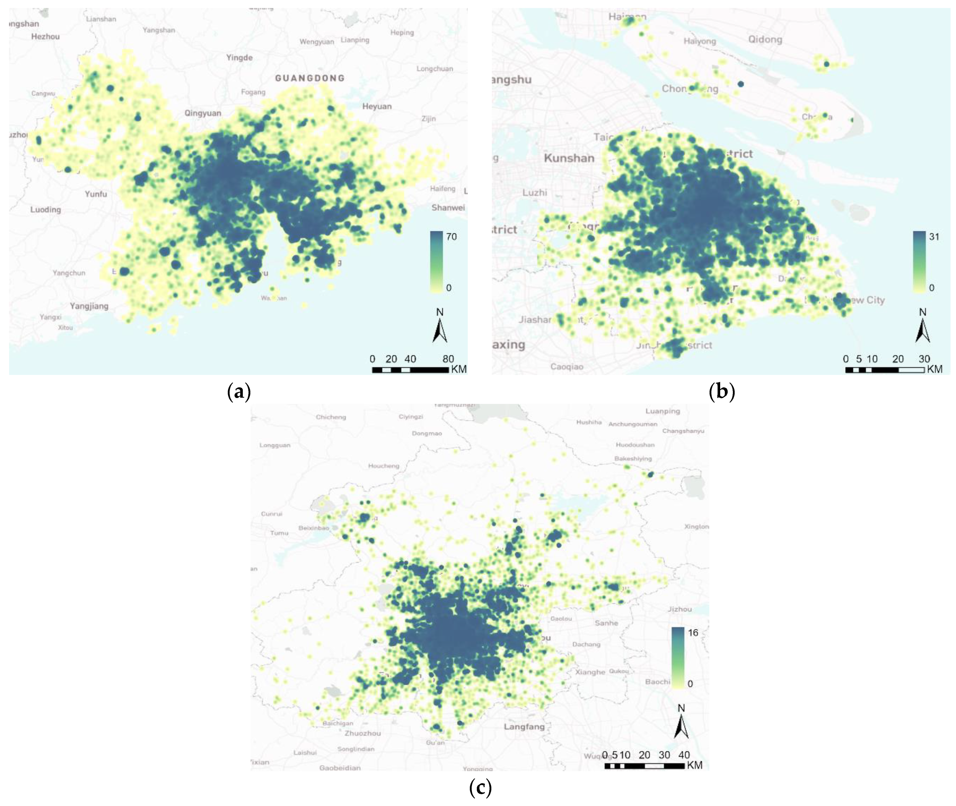
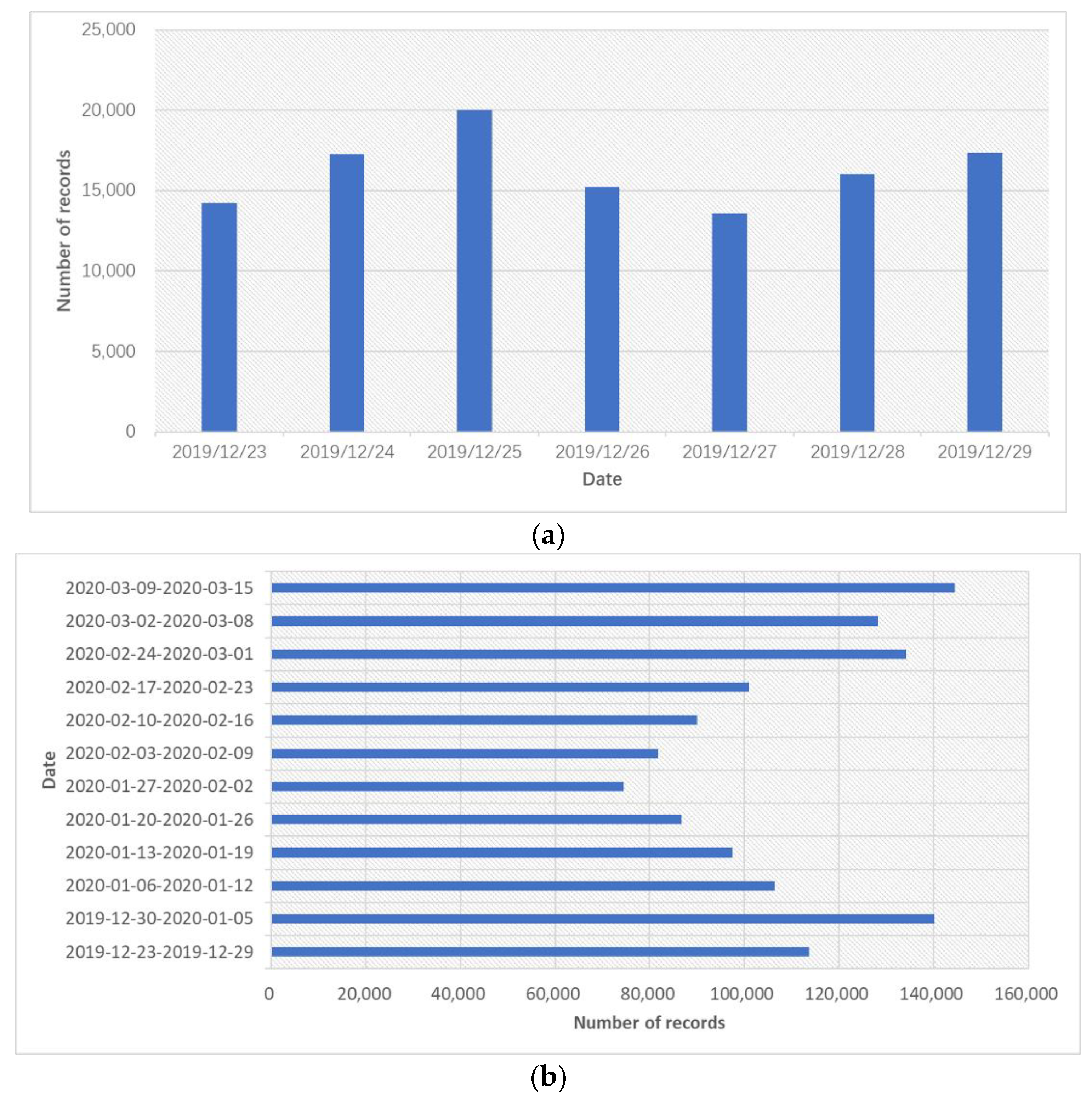
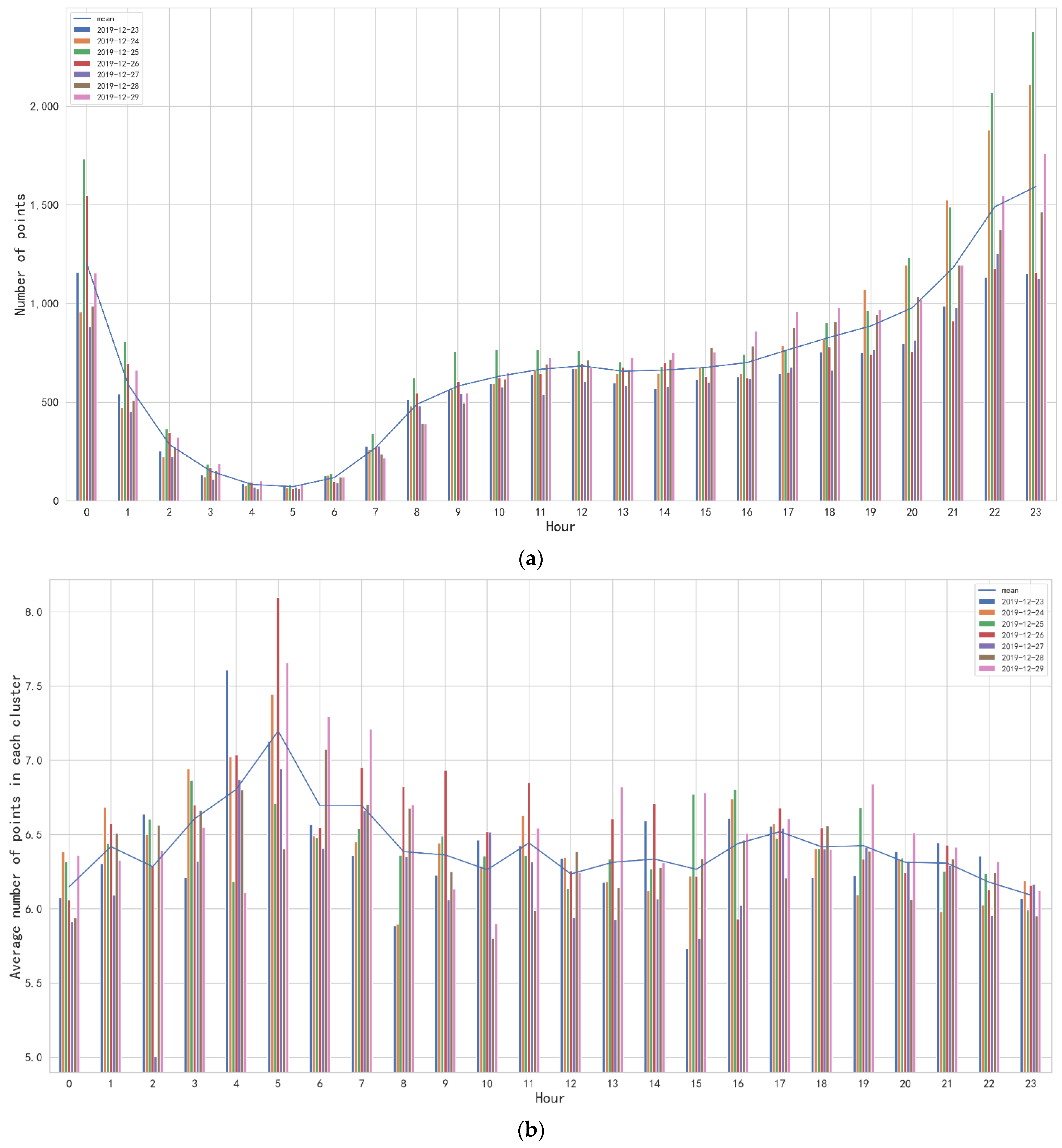
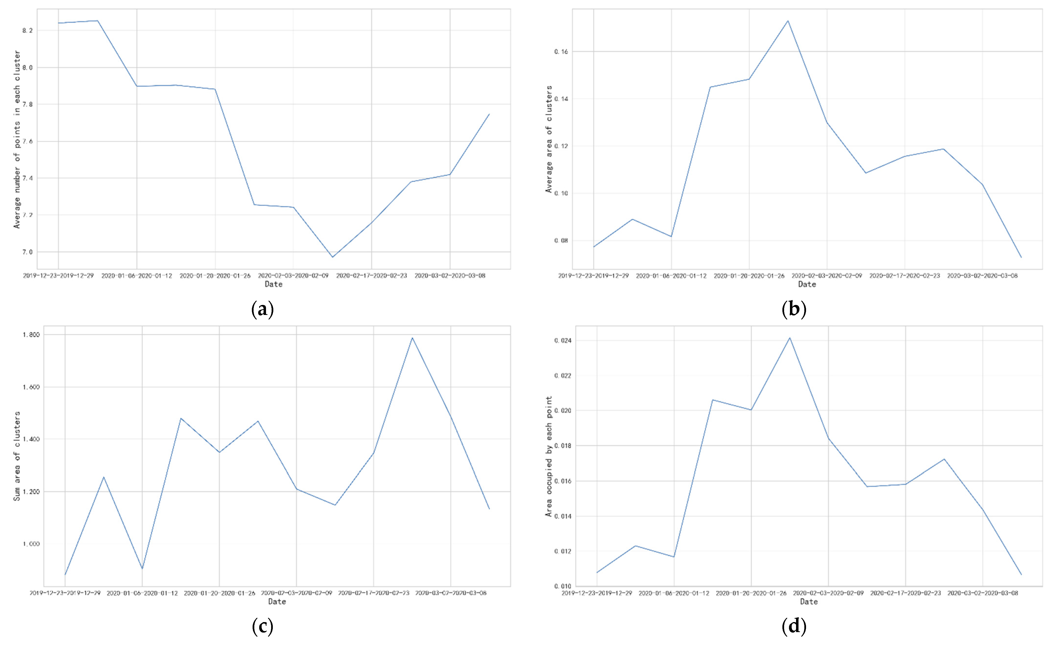
3.1. Data Description

Three real-life datasets, obtained from a social media platform (Weibo), were used in this research. The datasets were collected in different areas, including Guangdong–Hong Kong–Macao Greater Bay Area (the Greater Bay Area, GBA), Shanghai, and Beijing. The GBA dataset was extracted from an open dataset and can be found in [53]. Shanghai and Beijing are important and famous cities in China, especially Beijing, which is the capital of China. GBA is an urban agglomeration with 11 cities, including Hongkong, Macao, Shenzhen, Guangzhou, and others. According to

Table 1. Detailed information of the three datasets, showing the different spatio-temporal scales.

	GBA Dataset	Shanghai Dataset	Beijing Dataset
Time span	2019-12-23 to 2020-03-15	2020-7-6 to 2020-7-12	2019-12-23 to 2019-12-29
Space span	56,097 km2	6340 km2	16,410 km2
Number of cities	11	1	1
Total records	1,299,106	79,655	105,254

, the GBA dataset had the longest time span with 12 weeks, and the other two datasets both had a time span of one week. Because the GBA data covered 11 cities and the other two datasets only covered one city, the space span of the GBA dataset was several times that of the other two datasets, which was also reflected in the total records.

The spatial distribution characteristics of the three datasets are also shown in Figure 1. According to the heatmaps, the spatial distributions were very different. The GBA datasets (Figure 1a) had several large core areas with high densities, and some small areas with high densities distributed around the core areas. These high-density areas were mainly around the city centers, and the distributions in each city were different. Almost all areas in some cities had high densities, but only the centers of other cities had high densities. The Shanghai and Beijing datasets both had large core areas with very high densities, and areas with low densities were around the core areas.

Additionally, we not only used the whole GBA dataset but also extracted 7 days from the first week and the whole 12 weeks. The statistical information is shown in Figure 2. The number of records of the 7 days showed obvious differences: the number firstly increased and reached a peak on 25 December (Christmas Day), and then started to decrease until the weekend (28 and 29 December). According to Figure 2b, the number of records in the week (from 2019-12-30 to 2020-01-05) was very large due to New Year’s Day. However, during the Spring Festival, there were the least records. The reason for this may have been that individuals in these 11 cities returned home during the Spring Festival and could not go back to these cities due to COVID-19. The number then increased to large values due to the resumption of work.

In summary, the whole GBA dataset, Shanghai dataset, Beijing dataset and different parts of the GBA dataset were used in the experiment.

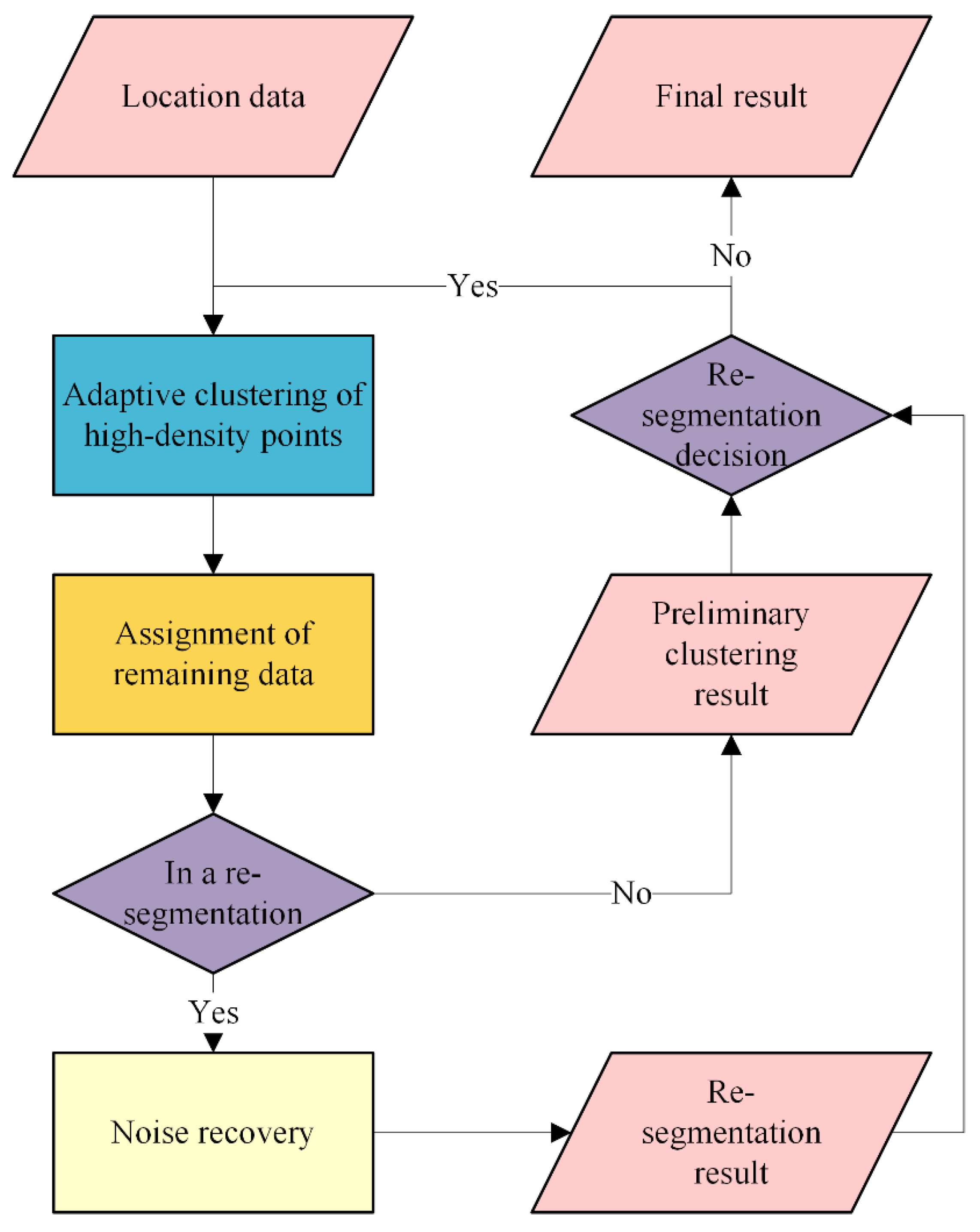
3.2. Extracting Human Activity Areas from Large-Scale Spatial Data with Varying Densities

In this research, the locations of human activity data were used for activity area extraction. The raw locations were represented by geodetic coordinates and transformed into plane coordinates. In the proposed framework, ELV, the new location data are processed by the following steps (shown in Figure 3):

(1)

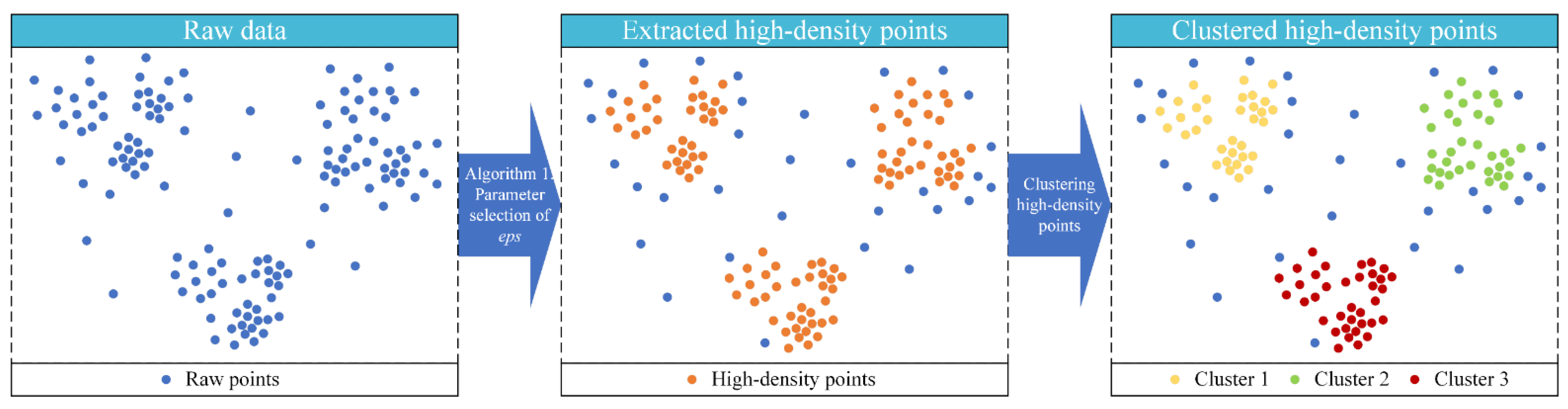
Adaptive clustering of high-density points. A distance parameter adaptive method is proposed to calculate the density of the points in the location data. The high-density points are then extracted as core points. The distance parameter is used to divide the core points into different clusters.

(2)

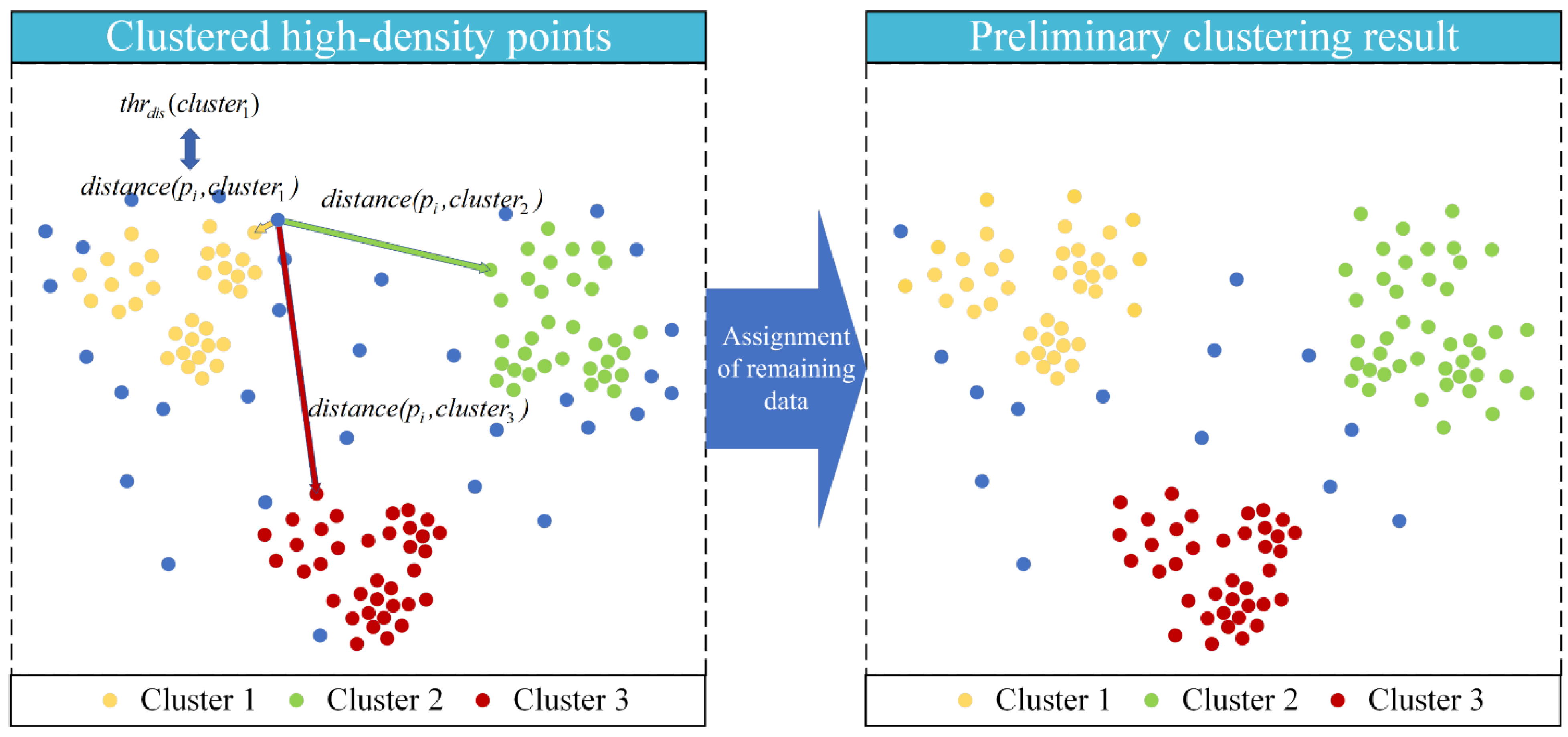
Assignment of remaining data. The spatial features of the core point clusters are extracted, which can describe the tightness of the core points in each cluster. Then, the features are combined into a distance threshold. For a remaining point, the nearest core point cluster is found, and the distance between them is compared with the distance threshold for point assignment.

(3)

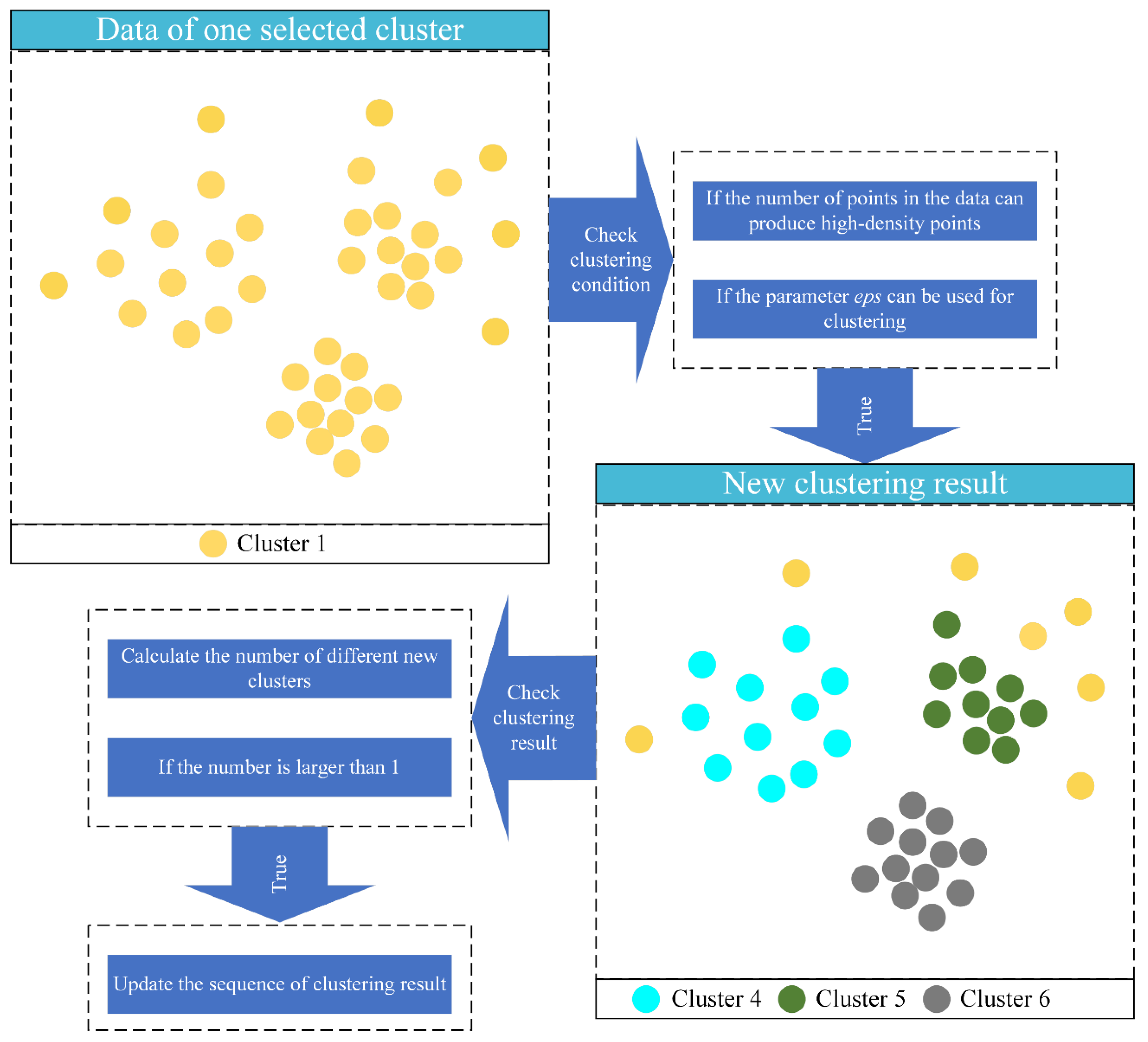
Re-segmentation decision. The preliminary clustering result obtained from the above two steps is used for the re-segmentation decision. Specifically, the number of points in a cluster is firstly used to decide if this cluster can be re-segmented. Then, the points are clustered again, and the distance parameter, the number of new clusters, and the noise points are used to decide if the re-segmentation is suitable.

(4)

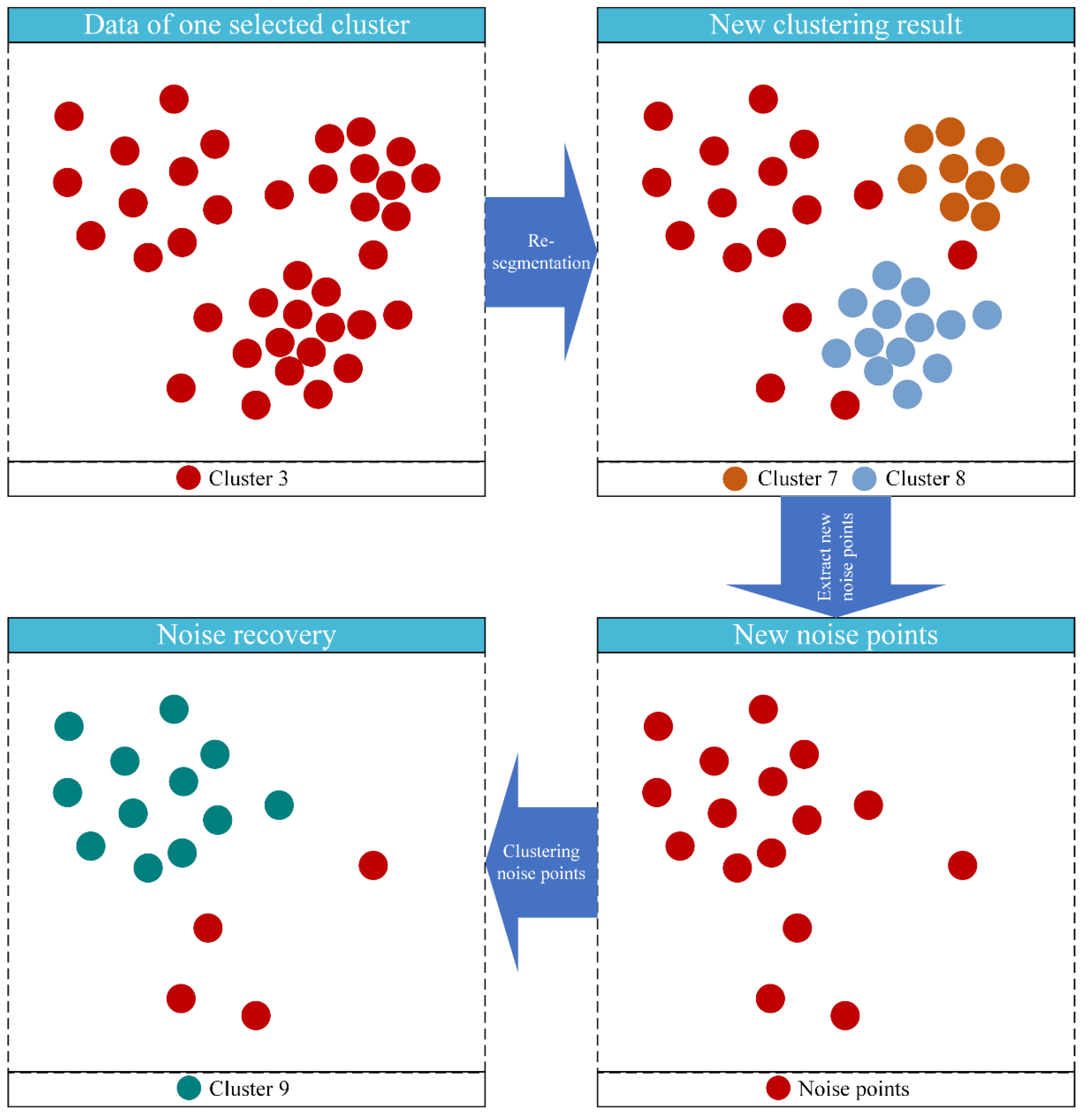
Noise recovery. In the re-segmentation step, the points in clusters may be considered noise, and as a result, too many noise points may be produced. Therefore, for each re-segmentation, the new noise points are re-clustered according to the old distance parameter, which has assigned them into a cluster, and the new distance parameter extracted from the noise points.

After the four main steps, the final result can be obtained, and the details of the four steps will be introduced below.

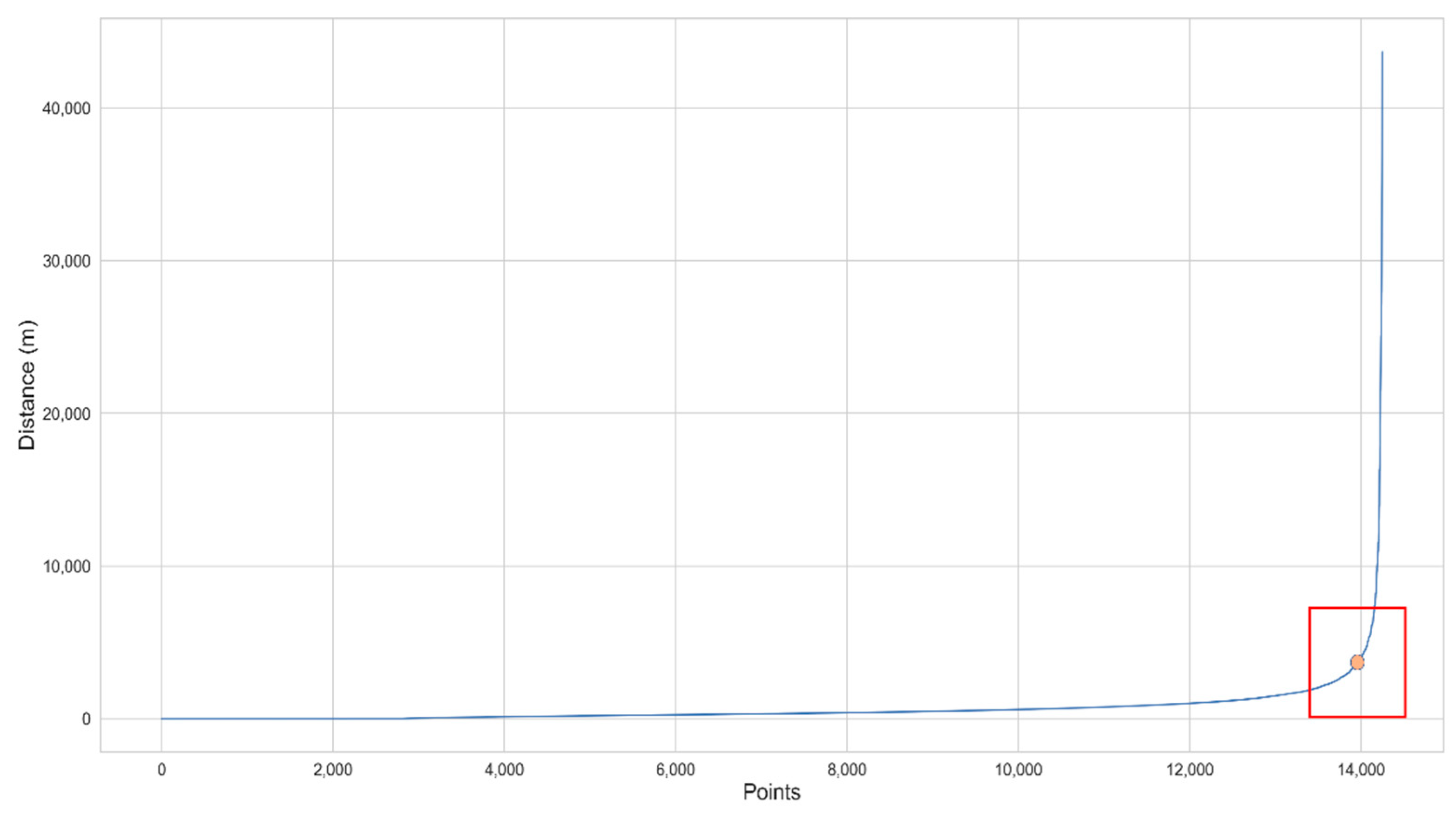
3.2.1. Adaptive Clustering of High-Density Points

In the whole proposed framework, the high-density points are firstly extracted and clustered. Therefore, a suitable definition of high density for the points in human activity data is necessary. Commonly, the density of a point is calculated as the number of points in a special range. This range is usually a circle with the point as the center, and the radius is artificially specified. Then, the problem of the calculation of the density is transformed into the selection of the radius, which is called $eps$ in other methods. In traditional applications, different values of $eps$ are tested, and users try to find the best value according to the results. However, it is hard to select a good result for large-scale data, and any selection may suffer from their low efficiency, especially for more than one dataset. A suggested method is to draw the k-distance graph, which can describe the relationships of the distances between different points. Here, $k$ is commonly set to twice the dimensions, and for spatial data with two dimensions, $k$ is 4. In detail, for a point, the distances between it and other points are calculated to find the $k$-th nearest point, and the distance is recorded. After obtaining the distances between all the points and their $k$-th nearest points, the distances are sorted as a sequence from small to large and can be defined as follows:

$$se{q}_{di{s}_k}\left(P\right)=\left[di{s}_k\left(p_1\right),di{s}_k\left(p_2\right),\cdots ,di{s}_k\left(p_i\right),\cdots ,di{s}_k\left(p_n\right)\right]$$

(1)

where $P$ refers to the dataset with $n$ points; $p_i$ are the points in $P$; $di{s}_k\left(p_i\right)$, with $1\le i\le n$, is a function to calculate the distance between $p_i$ and the $k$-th nearest point; $se{q}_{di{s}_k}\left(P\right)$ is the sorted distance sequence. Then, the sequence can be drawn as shown in Figure 4, with distances on the vertical Y-axis against points on the horizontal x-axis. From the example figure, the curve changed around 14,000, and we selected the orange point as the elbow point, whose distance can be considered as $eps$. However, it should be noted that the selection was subjective, and the points in the red box may be considered elbow points by different people.

We proposed an adaptive method to extract the elbow from the figure to reduce subjective factors (shown in Algorithm 1). Indeed, it is hard to use mathematical formulas to represent the curve, but this problem can be solved from a geometric point of view. Observing the figure, it can be easily found that the curvature around the elbow point was large, while it was small at other points. Therefore, we can try to describe the curvatures mathematically and then extract the point max curvature. After obtaining sorted $se{q}_{di{s}_k}(P)$ (Algorithm 1 line 1–5), the angles of every three points are used to represent curvatures and the sequence of angles can be defined as follows (Algorithm 1 line 6–9):

Algorithm 1: Parameter selection of $eps$

Input: All the points for clustering $P$

Output: $eps$

$se{q}_{di{s}_k}\left(P\right)$ = [ ] for $p_i$ in $P$: $\hspace{1em} di{s}_k\left(p_i\right)$ = Distance ($p_i$, k)//calculate the distance between $p_i$ and the k-th nearest point $\hspace{1em} se{q}_{di{s}_k}\left(P\right)$.append($di{s}_k\left(p_i\right)$) sort($se{q}_{di{s}_k}\left(P\right)$) $se{q}_{ang}\left(P\right)$ = [ ] for $di{s}_k\left(p_i\right)$ in $se{q}_{di{s}_k}\left(P\right)$: $\hspace{1em} ang\left(p_{i-2},p_{i-1},p_i\right)=ang\left(\overrightarrow{p_{i-1}{p}_{i-2}},\overrightarrow{p_{i-1}{p}_i}\right)$//calculate the angle of three continuous points $\hspace{1em} se{q}_{ang}\left(P\right)$.append($ang\left(p_{i-2},p_{i-1},p_i\right)$) $p_{elbow}$ = [ ] for $size$ in range(1, $siz{e}_{max}$): $\hspace{1em}{p}_{elbow}$.append($argmin\left(smoot{h}_{size}\left(se{q}_{ang}\left(P\right)\right)\right)$)//extract the elbow points $p_{elbow}$ = mean($p_{elbow}$) $eps$ = $di{s}_k\left(p_{elbow}\right)$ return $eps$

$$se{q}_{ang}\left(P\right)=\left[ang\left(p_1,p_2,p_3\right),ang\left(p_2,p_3,p_4\right),\cdots ,ang\left(p_{i-2},p_{i-1},p_i\right),\cdots ,ang\left(p_{n-2},p_{n-1},p_n\right)\right]$$

(2)

where $se{q}_{ang}\left(P\right)$ is the function to obtain the sequence of angles, and $ang\left(p_{i-2},p_{i-1},p_i\right)$ is used to calculate the angle of three continuous points. This is based on the coordinates in the $k$-distance graph, instead of the raw coordinates in the real world. The coordinate of a point $p_i$ is the $\left(i,di{s}_k\left(p_i\right)\right)$ and the angle function can be defined as follows (Algorithm 1 line 8):

$$ang\left(p_{i-2},p_{i-1},p_i\right)=ang\left(\overrightarrow{p_{i-1}{p}_{i-2}},\overrightarrow{p_{i-1}{p}_i}\right)$$

(3)

where $\overrightarrow{p_{i-1}{p}_{i-2}}$ and $\overrightarrow{p_{i-1}{p}_i}$ are the vectors combined by the three points, and the angle refers to the included angle of the two vectors. The point with the largest curvature is the mid-point of the three points with the smallest angle:

$$p_{elbow}=argmin\left(se{q}_{ang}\left(P\right)\right)$$

(4)

There is still the problem that the curve may be not smooth enough, leading to the wrong extraction of the elbow point. To enhance the reliability of the method, sliding windows with different sizes from 1 to $siz{e}_{max}$ are used on $se{q}_{ang}\left(P\right)$, and new smoothed sequences of angles can be obtained, recorded as $smoot{h}_{size}\left(se{q}_{ang}\left(P\right)\right)$ where $1\le size\le siz{e}_{max}$. The new values of the angles in the smoothed sequences are as follows:

$$an{g}_{size}\left(p_{i-2},p_{i-1},p_i\right)=avg\left(\begin{array}{c}ang\left(p_{i-2-size/2},p_{i-1-size/2},p_{i-size/2}\right),\\ \cdots ,ang\left(p_{i-2},p_{i-1},p_i\right),\\ \cdots ,ang\left(p_{i-2+size/2},p_{i-1+size/2},p_{i+size/2}\right)\end{array}\right)$$

(5)

which calculates the average value of the angles in the sliding window. The final elbow point can be defined as follows (Algorithm 1 line 10–13):

$$p_{elbow}=\frac{{\displaystyle \sum _{size=1}^{siz{e}_{\mathit{max}}}argmin\left(smoot{h}_{size}\left(se{q}_{ang}\left(P\right)\right)\right)}}{siz{e}_{\mathit{max}}}$$

(6)

Then, the value of $siz{e}_{max}$ should be suitably selected, because a too large $siz{e}_{max}$ may lead to distortions in the curve. Therefore, let $siz{e}_{max}=n\ast th{r}_{size}+1$, where $th{r}_{size}$ is a percent of the whole data size. The value of $th{r}_{size}$ can be set as a very small constant (1%) to keep the reliability of the smoothed sequence. Then, a cutoff value $n_{cutoff}=1/th{r}_{size}$ appears. If the size of points is smaller than $n_{cutoff}$, $siz{e}_{max}$ is always 1 and the smooth function does not work. Therefore, we set the smallest value of $siz{e}_{max}$ as 2. However, when the size of points is too large ($n\gg n_{cutoff}$), the calculation loop of the smoothed sequence will be huge. This does not influence the effectiveness of the method theoretically, but the efficiency may be low in practical application. Another threshold is set to limit the number of loops. For a dataset with $n_{cutoff}$ points, the size of the sliding window should at least be smaller than $n_{cutoff}/2$ to make the amount of valid data greater (recorded as $am\left(vd\right)$) than that of invalid data (recorded as $am\left(id\right)$). For a dataset with $n$ points ($n\gg n_{cutoff}$), $am\left(vd\right)\gg am\left(id\right)$ if the size is still $n_{cutoff}/2$. Therefore, $siz{e}_{max}$ can be defined as follows:

$$siz{e}_{max}=\mathit{max}\left(\begin{array}{c}2\\ \min \left(\begin{array}{c}n\ast th{r}_{size}+1\\ \frac{n_{cutoff}}{2}\end{array}\right)\end{array}\right)$$

(7)

After the automatic extraction of $eps$, the high-density points can be extracted and clustered (shown in Figure 5). Firstly, the densities of the points are calculated, and high-density points, with densities no smaller than $k$, are extracted (colored orange in the middle figure of Figure 5). The clustering process of high-density points is then started. The core idea is to make the distances between points in a cluster smaller than $eps$, and the distances between clusters larger than $eps$. Therefore, the first point is randomly selected and set as the first cluster. All the high-density points, with distances between them and any one point in the cluster smaller than $eps$, belong to the cluster and should be labeled with a number. Then, the process is cycled on the remaining points until all high-density points belong to some clusters and are labeled. In the right part of Figure 5 three different clusters with high-density points were extracted. Finally, a set of clusters ($cluste{r}_1,cluste{r}_2,\cdots ,cluste{r}_j,\cdots ,cluste{r}_m$,$1\le j\le m$) and a cluster label sequence of the points ($cl(P)$) can be obtained:

$$cl\left(P\right)=\left[labe{l}_1,labe{l}_2,\cdots ,labe{l}_i,\cdots ,labe{l}_n\right]$$

(8)

The low-density points are not labeled in the above clustering process (still colored with blue in the right figure of Figure 5), but for convenience they are all labeled with −1 and will be clustered in the next part.

3.2.2. Assignment of Remaining Data

All the high-density points are clustered in the above process, and the remaining points are tried to be assigned to the clusters (Algorithm 2). Figure 6 shows an example of the assignment. There are two main steps for the assignment, namely finding the most possible cluster and judging if the points meet the cluster features. In the first step, the possibility of a point belonging to a cluster is evaluated by the distance between them (Algorithm 2 line 7–9). In the example, distances between the selected point and three clusters are calculated. The smaller the distance, the greater the possibility. The process of a point ($p_i$) is as follows:

$$j=\underset{1\le j\le m}{argmin\left(distance\left(p_i,cluste{r}_j\right)\right)}$$

(9)

The distance between a point and a cluster can be defined in different formats. One method is to use a point, such as the centroid of the cluster, to represent the cluster. Another method uses the mean value of all the distances between the target point and all the points in the cluster. The methods can work well on clusters of convex shapes, but in this research, shapes of the clusters obtained based on density can be irregular. Therefore, only the min value of the distances between the target point and all the points in the cluster is used. Combined with Equation (8), the process to find the most possible cluster can be simplified to find the cluster with the nearest point.

Algorithm 2: Assignment of remaining data

Input: Clustering result of high-density points $cl\left(P\right)$

Output: Preliminary clustering result recorded in updated $cl\left(P\right)$

for $j$ in range(m): $\hspace{1em}data\left(cluste{r}_j\right)$ = extracted($cl\left(P\right)$,$j$)//extract related points according to the labels $\hspace{1em}dis\left(cluste{r}_j\right)$ = [ ]  for point in $data\left(cluste{r}_j\right)$: $\hspace{1em}\hspace{1em}dis\left(cluste{r}_j\right)$.append(mindistance(point))//calculate the distance between each point and its nearest point in $cluste{r}_j$ $\hspace{1em}th{r}_{dis}\left(cluste{r}_j\right)=mean\left(dis\left(cluste{r}_j\right)\right)+3\ast std\left(dis\left(cluste{r}_j\right)\right)$//calculate the distance threshold for $labe{l}_i$ in $cl\left(P\right)$:  if $labe{l}_i$ != −1: continue//skip the labeled points $\hspace{1em}j=\underset{1\le j\le m}{argmin}\left(distance\left(p_i,cluste{r}_j\right)\right)$//find the most possible cluster  if $distance\left(p_i,cluste{r}_j\right)\le th{r}_{dis}\left(cluste{r}_j\right)$: $\hspace{1em}\hspace{1em}labe{l}_i$ = $j$ $\hspace{1em} cl\left(P\right)$.update($labe{l}_i$) return $cl\left(P\right)$

In the second step, we judge if a point belongs to the most possible cluster according to $distance\left(p_i,cluste{r}_j\right)$ and a distance threshold ($th{r}_{dis}$) (Algorithm 2 line 10–12). In Figure 6, the most possible cluster is Cluster 1, so $distance\left(p_i,cluste{r}_1\right)$ and $th{r}_{dis}\left(cluste{r}_1\right)$ are compared. The value of $eps$ is often used as the threshold in other methods, but this ignores the different spatial features of the clusters. For example, there are two points and their most possible clusters. The points in one cluster are very concentrated, and the area of the cluster (such as a convex hull) is very small. An extreme case is that all the points are with the same coordinate. For this case, even if $distance\left(p_i,cluste{r}_j\right)$ is smaller than $eps$, the point is still not suitable to be assigned to the cluster. In another cluster, the distribution of the points is scattered, and the distances between the points are near to $eps$. The assignment of the point to this cluster is thus very suitable. Therefore, varying thresholds are set according to the spatial distribution of the points in the most possible clusters.

A part of the distances between the points in a most possible cluster is used to describe the spatial distribution (Algorithm 2 line 1–6). The reason why not all the distances are used is that the shapes in this research are irregular, and distances between some points may be very large. For each point in the cluster, the distance between it and the nearest point in the cluster is calculated. Then, a distance group of the cluster ($dis\left(cluste{r}_j\right)$) can be obtained to describe the spatial distribution. The max value in the group is recorded as $max\left(dis\left(cluste{r}_j\right)\right)$, the mean value is recorded as $mean\left(dis\left(cluste{r}_j\right)\right)$, and the standard deviation is recorded as $std\left(dis\left(cluste{r}_j\right)\right)$. The distance threshold of a cluster ($th{r}_{dis}\left(cluste{r}_j\right)$) is defined as follows:

$$th{r}_{dis}\left(cluste{r}_j\right)=mean\left(dis\left(cluste{r}_j\right)\right)+3\ast std\left(dis\left(cluste{r}_j\right)\right)$$

(10)

In the above equation, the triple standard deviation is used to statistically remove noise. A value range of $th{r}_{dis}\left(cluste{r}_j\right)$ should be set to enhance the robustness of the method. The points in a cluster sometimes may have an uneven distribution, and some closely distributed points can lead to a small $th{r}_{dis}\left(cluste{r}_j\right)$, which can produce too much noise. Therefore, $max\left(dis\left(cluste{r}_j\right)\right)$ is set to the lower limit, and if $th{r}_{dis}\left(cluste{r}_j\right)$ is smaller than $max\left(dis\left(cluste{r}_j\right)\right)$, let $th{r}_{dis}\left(cluste{r}_j\right)=max\left(dis\left(cluste{r}_j\right)\right)$. The upper limit is set to $eps$ to ensure the filter of noise points, and if $th{r}_{dis}\left(cluste{r}_j\right)$ is larger than $eps$, let $th{r}_{dis}\left(cluste{r}_j\right)=eps$. These thresholds of different clusters can be calculated at the beginning as described in Algorithm 2 line 1–6 for efficiency. At last, the label of a remaining point ($labe{l}_i$) can be defined as follows:

$$labe{l}_i=\{\begin{array}{c}jifdistance\left(p_i,cluste{r}_j\right)\le th{r}_{dis}\left(cluste{r}_j\right)\\ -1ifdistance\left(p_i,cluste{r}_j\right)>th{r}_{dis}\left(cluste{r}_j\right)\end{array}$$

(11)

After obtaining all the point labels according to Equation (11), the elements in Equation (8) are then changed into corresponding labels (Algorithm 2 line 10–13) and a preliminary clustering result is obtained (right part of Figure 6).

3.2.3. Re-Segmentation Decision

The preliminary clustering result recorded in $cl(P)$ is then used for re-segmentation in order to address the varying density problem of large-scale spatial data. The process flow of one re-segmentation is described in Algorithm 3 and Figure 7 shows the re-segmentation on a selected cluster. In this step, each cluster in $cl\left(P\right)$ is extracted with its labels and coordinates as a new dataset $data\left(cluste{r}_j\right)$ (Algorithm 3 line 1–2). Then, the above two clustering steps (Section 3.2.1 and Section 3.2.2) are processed on the new dataset again, and the clustering result ($cl\left(data\left(cluste{r}_j\right)\right)$) is used to update the elements in $cl\left(P\right)$. After all the clusters have been processed, the re-segmentation is circularly used on the updated $cl\left(P\right)$. In the loop, there are two main problems that need to be addressed, namely if $data\left(cluste{r}_j\right)$ can be clustered (Algorithm 3 line 3–9) and if $cl\left(data\left(cluste{r}_j\right)\right)$ is a good result to update $cl\left(P\right)$ with (Algorithm 3 line 10–16).

Firstly, $data\left(cluste{r}_j\right)$ is checked to see if it can be clustered, and Cluster 1 is selected in Figure 7. According to Section 3.2.1, the high-density points should be extracted and clustered. Therefore, the basic cluster condition is that there is at least one high-density point, which means the number of points in $data\left(cluste{r}_j\right)$ should not be smaller than k (Algorithm 3 line 3–4). If the number meets the condition, the adaptive method of $eps$ extraction is used on the points to obtain a new value ($ep{s}_j$). The value of $ep{s}_j$ is compared with the old value $eps$, which was used to produce $cluste{r}_j$. If $ep{s}_j$ is not smaller than $eps$, the re-segmentation does not make sense (Algorithm 3 line 5–7). Then, $data\left(cluste{r}_j\right)$ is clustered by the method in Section 3.2.1 and Section 3.2.2 using the parameter $ep{s}_j$.

Secondly, the clustering result $cl\left(data\left(cluste{r}_j\right)\right)$ is checked to see if is good to update $cl\left(P\right)$ with. The number of different labels in $cl\left(data\left(cluste{r}_j\right)\right)$ is calculated and if there is any noise let the number minus 1 (Algorithm 3 line 10–12). This number can describe the counts of valid activity areas in this re-segmentation and is checked to see if is larger than 1. In Figure 7, Cluster 1 is divided into three new clusters and the new clustering result is suitable to update $cl\left(P\right)$. However, when the number is 1, the re-segmentation cannot extract new clusters and just produces more noise points. Such a situation makes no sense for activity area extraction and $cl\left(P\right)$ should not be updated with $cl\left(data\left(cluste{r}_j\right)\right)$. Different values of $ep{s}_j$ from $eps$ to 0 are additionally tried to enhance the stability of results on data with a very small number of points when the return of Algorithm 3 is −1. The clustering results continue to be checked until the number of labels is larger than 1, which means loop the processing of Algorithm 3 line 8–16 with different $ep{s}_j$. If none result can meet the condition, $cl\left(P\right)$ is not updated in this re-segmentation.

Algorithm 3: Re-segmentation once

Input: Preliminary clustering result $cl\left(P\right)$, parameter $eps$

Output: Re-segmentation result recorded in updated $cl\left(P\right)$

for $j$ in range(m): $\hspace{1em}data\left(cluste{r}_j\right)$ = extracted($cl\left(P\right)$,$j$)//extract related points according to the labels  if len($data\left(cluste{r}_j\right)$) < k:   return 0//check if the number of points in the data can be clustered $\hspace{1em}ep{s}_j$ = Algorithm 1($data\left(cluste{r}_j\right)$)  if $ep{s}_j$ ≥ $eps$://check if the paramter can be used for clustering   return −1 $\hspace{1em}cl\left(data\left(cluste{r}_j\right)\right)$ = cluster_high_density_points($data\left(cluste{r}_j\right)$,$ep{s}_j$) $\hspace{1em}cl\left(data\left(cluste{r}_j\right)\right)$ = Algorithm 2($cl\left(data\left(cluste{r}_j\right)\right)$)  num_labels = len(unique($cl\left(data\left(cluste{r}_j\right)\right)$))//calculate the number of different labels  if −1 in $cl\left(data\left(cluste{r}_j\right)\right)$:   num_labels = num_labels − 1  if num_labels ≤ 1:   return −1//check if the cluster result can be used for updating $\hspace{1em}cl\left(P\right)$.update($cl\left(data\left(cluste{r}_j\right)\right)$) return $cl\left(P\right)$

Using the above two check steps, new $cl\left(P\right)$ can be obtained, and one re-segmentation ends. The two steps (Algorithm 3) continue to cycle on the new $cl\left(P\right)$ until there are no qualified results. To improve the efficiency of the loop, a label set can be used to record the labels whose corresponding points need to be re-segmented. If points in a cluster cannot meet the above two checks, the label of this cluster is removed from the label set. Additionally, once points in a cluster are re-segmented, the old label is removed, and new labels different from existing labels in the label set should be added.

3.2.4. Noise Recovery

This section introduces the strategy to recover the noise points in the re-segmentation step (Algorithm 4). Many exiting methods do not generate noise points, but for human activity area extraction it is necessary due to the randomness of human mobility. Density-based methods usually divide points into noise according to density and the distance between points. For these methods, noise recovery is not needed, because they only produce noise points once. However, the loop in the re-segmentation step continues to cluster points, and can produce more noise points than other methods. Some applications only focus on several high-density areas, such as hotspots, and lots of points with no high densities are considered noise. In such a situation, noise recovery makes no sense. In this research, we tried to extract human activity areas with varying densities. In a re-segmentation loop, the points with relatively small densities may be considered noise, even though they have been clustered in the previous loop, and such points are the objects of the noise recovery. In Figure 8, the points of Cluster 3 were divided into two clusters and lots of points are considered noise due to the density difference. Some of the noise points can be recovered by a larger parameter.

The principle of noise recovery is similar to the two conditions which judge if the points can be re-segmented. The recovery process is added after the re-segmentation of each cluster data ($data\left(cluste{r}_j\right)$). The noise points are extracted from the clustering result ($cl\left(data\left(cluste{r}_j\right)\right)$) (Algorithm 4 line 1–4). Then, an adaptive distance parameter, recorded as $ep{s}_{noise}$, can be calculated if the number of noise points is larger than $k$ (Algorithm 4 line 5–7). There are now three different values of the distance parameter, namely the value which divides these points into a cluster ($eps$), the value which considers the points as noise ($ep{s}_j$), and the new value which tries to cluster the points again ($ep{s}_{noise}$). According to Section 3.2.3, $ep{s}_j$ is smaller than $eps$, and if $ep{s}_{noise}\le ep{s}_j$, these points are still noise, so the lower limit of $ep{s}_{noise}$ is $ep{s}_j$. When $ep{s}_{noise}$ is large enough, these points, even with huge distances between them, still can be clustered. This is not suitable for practical applications, and therefore an upper limit is set to $eps$ (Algorithm 4 line 8–9).

Then, the noise points can be clustered using $ep{s}_{noise}$ based on the steps introduced in Section 3.2.1 and Section 3.2.2. The result $c{l}_{noise}\left(data\left(cluste{r}_j\right)\right)$ is used to update the elements in $cl(P)$, but the new labels of the noise points do not need to be added into the label set. The reason for this is that there has been a lower limit of $ep{s}_{noise}$, which means the cluster cannot be re-segmented.

Algorithm 4: Noise recovery

Input: Clustering result $cl\left(data\left(cluste{r}_j\right)\right)$, parameters $eps$ and $ep{s}_j$

Output: Clustering result of noise data $c{l}_{noise}\left(data\left(cluste{r}_j\right)\right)$

noise_points = [ ] for point in $cl\left(data\left(cluste{r}_j\right)\right)$:  if point is noise:   noise_points.append(point)//extract noise points for recovery from $cl\left(data\left(cluste{r}_j\right)\right)$ if len(noise_points) < k:  return 0//check if the number of points in the noise data can be clustered $ep{s}_{noise}$ = Algorithm 1(noise_points) if $ep{s}_{noise}$ ≤ $ep{s}_j$ or $ep{s}_{noise}$ ≥ $eps$://check if the paramter can be used for clustering   return −1 $c{l}_{noise}\left(data\left(cluste{r}_j\right)\right)$ = cluster_high_density_points(noise_points, $ep{s}_{noise}$) $c{l}_{noise}\left(data\left(cluste{r}_j\right)\right)$ = Algorithm 2($c{l}_{noise}\left(data\left(cluste{r}_j\right)\right)$) return $c{l}_{noise}\left(data\left(cluste{r}_j\right)\right)$

3.3. Clustering Algorithms for Comparison

To verify the effectiveness of the proposed framework, ELV, three existing methods were also tested, namely, density peak clustering (DPC) [25], density-based spatial clustering of applications with noise (DBSCAN) [4,23,24], and Hierarchical DBSCAN (HDBSCAN) [5,27,28,29]. As introduced in Section 1 and Section 2, DPC is a simple and effective clustering algorithm that was proposed recently and has been applied in many fields. DBSCAN is a very famous and popular clustering algorithm, and many researchers use it for human activity area extraction. HDBSCAN improves DBSCAN by introducing the hierarchical clustering idea, and has been proved effective in clustering spatial data. The basic principles and the parameter selections of the three methods are as follows:

• DPC: This algorithm introduces the idea that cluster centers have higher densities than the points around them and the distances between centers are large. Therefore, the algorithm clusters data by extracting points, meeting the idea, as cluster centers, and then assigning other points to the centers. It has two parameters that need to be selected manually, including $dis$ and $den$. A point with a density larger than $den$ is considered a high-density point and high-density points with distances between them larger than $dis$ are cluster centers. This algorithm also provides a method to set the parameters according to the distribution graphs of density and distance. Therefore, we set the parameters according to the method in the paper for each dataset, and mainly the $dis$ and $den$ were set to 7000 and 50.
• DBSCAN: Core points are defined in this algorithm according to the number of points in the neighborhoods. As shown in

  Table 2. Parameters with their descriptions and values of the three algorithms.

  Algorithm	Parameter	Description	Value
  DPC	$dis$	distance threshold used to extract cluster centers	7000
  	$den$	density threshold used to extract cluster centers	50
  DBSCAN	$minpts$	min number of points in neighborhoods of core points	4
  	$eps$	distance to define the size of neighborhoods	200, 400, 800, and 1600
  HDBSCAN	$mcs$	minimum cluster size	4, 8, 16, and 32

  a core point has at least $minpts$ points with the distance between them smaller than $eps$. For each core point, find all other points in its neighborhoods and assign them to the same cluster. When a cluster has new core points, repeat the previous step. The parameter $minpts$ is set to twice the dimensions of the data, which is 4 in this research, according to the suggestion of the algorithm. Another parameter, $eps$, was set to different values: 200, 400, 800, and 1600.
• HDBSCAN: The data are first transformed into a new distance form based on the core distance to reduce the influence of noise. A minimum spanning tree is built to describe the data and transform the data into a cluster hierarchy by creating clusters for the edges in the spanning tree. The clusters with sizes smaller than $mcs$ are considered noises and then the cluster hierarchy tree can be condensed. At last, clusters can be extracted based on an index that measures the stabilities of clusters. The parameter, $mcs$, were set to different values in this research, including 4, 8, 16, and 32.

4. Results

The proposed framework, ELV, was tested using three real-life datasets and compared with three state-of-the-art methods, including DPC, DBSCAN, and HDBSCAN. In this section, the first-day data of the GBA dataset was used as an example to show the characteristics of clustering results of different algorithms. Then, the comparison results of the whole datasets were evaluated based on two indicators, and the extraction results of our framework were analyzed. Based on the visual analysis and two measurements, the experiment tested how the proposed framework, ELV, performed compared with other popular algorithms. Lastly, we discussed the experiment results of the algorithms to analyze the strengths and weaknesses.

In this research, the experiments and analysis were mainly based on Python, ArcGIS Pro [54], and Tableau [55]. We implemented our framework and other algorithms, based on Python with different libraries such as Pandas [56], Numpy [57], HDBSCAN [58], scikit-learn [59], and so on. The results were visualized and analyzed using ArcGIS Pro, Tableau, and other libraries such as Matplotlib [60] and Seaborn [61].

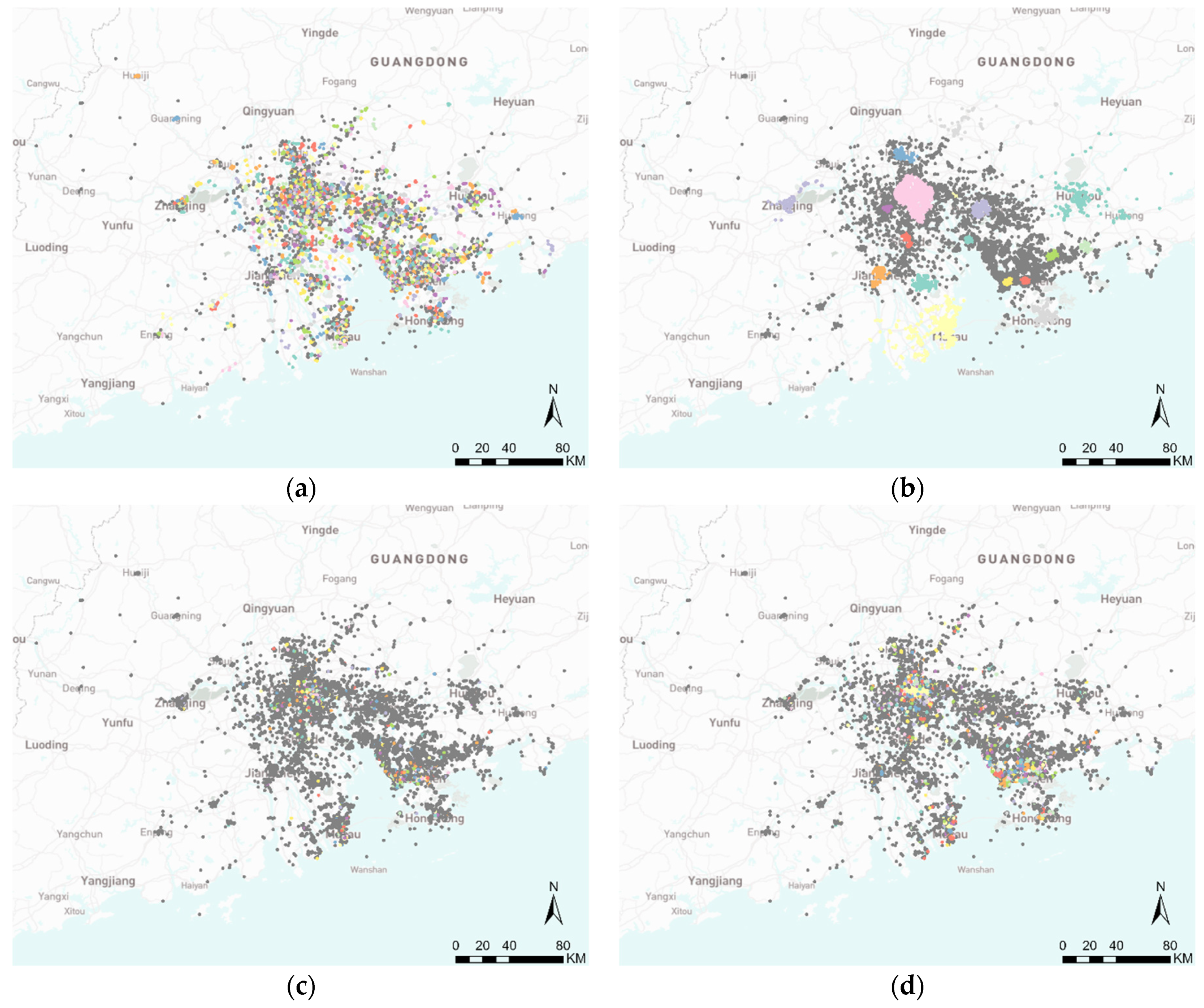
4.1. Performance Comparison Using the First-Day Data of the GBA Dataset as an Example

The first-day data of the GBA dataset, with 14,248 points, was selected as an example to show the basic cluster results of the different methods.

Table 3. Statistical information of the different methods tested on the first-day data in the GBA dataset.

Methods	Number of Clusters	Average Number of Points in Each Cluster	Clustered Points		Noise Points
			Number	Ratio	Number	Ratio
ELV	1660	6.78	11,252	78.97%	2996	21.03%
DPC	18	434.78	7826	54.93%	6422	45.07%
DBSCAN 200	586	9.60	5624	39.47%	8624	60.53%
DBSCAN 400	599	15.09	9041	63.45%	5207	36.55%
DBSCAN 800	422	28.11	11,863	83.26%	2385	16.74%
DBSCAN 1600	211	63.53	13,405	94.08%	843	5.92%
HDBSCAN 4	952	10.52	10,013	70.28%	4235	29.72%
HDBSCAN 8	405	21.34	8642	60.65%	5606	39.35%
HDBSCAN 16	172	45.46	7819	54.88%	6429	45.12%
HDBSCAN 32	68	107.88	7336	51.49%	6912	48.51%

describes the main statistical characteristics of the clustering results. Our proposed framework, ELV, obtained the largest number of clusters, and correspondingly the average number of points in each cluster was the smallest. HDBCAN 4 obtained the second largest number of clusters, but this was still much smaller than that of ELV. The smallest average number of points was 6.78, which was very small relative to the number of whole points (14,248) and also smaller than those of other methods. From the point of geographical space, the whole points were distributed in a total of 11 cities with 56,097 km² and the data was sparse for human activity area extraction, so each activity area just contains a small number of points. Therefore, the small sizes of clusters were relatively reasonable. The average value of points obtained by DBSCAN 200 and HDBSCAN were, respectively, 9.60 and 10.52, which were close to that of ELV. The differences in the values were mainly caused by the re-segmentation step which can divide large clusters into small ones. This reflected that ELV can better extract fine-grained activity areas from large-scale space data than other methods. Additionally, the ratios of clustered points of HDBSCAN with different parameters were all smaller than ELV. DBSCAN 200 and 400 produced too many noise points, and DBSCAN 800 and 1600 obtained a very small number of clusters. With the increase in the parameter, the average number of points in each cluster of DBSCAN also increased. This reflected the fact that DBSCAN clustered a lot of points in several clusters, and some noise points were assigned to clusters; as a result, it was unable to distinguish different activity areas. For example, the ratio of noise points generated by DBSCAN 1600 was 5.92%, the smallest one, but the number of clusters was 211, which meant only an average of 19.18 clusters in each city. This number of 19.18 was too small for human activity areas in a city compared with the actual human activities. Figure 9 showed that DBSCAN 800 and 1600 divided too many points into several clusters, which made no sense in some city centers for human activity area extraction. The problem with HDBSCAN was that too many points were assigned as noise and some possible activity areas could not be identified. The performance of DPC was the worst: it extracted only 18 clusters with 45.07% noise points. Our proposed framework not only extracted lots of fine-grained activity areas but also controlled the noise in a small ratio.

The visualizations of the results shown in Figure 9 also show the better performance of ELV compared with the other methods. ELV extracted lots of clusters in both low- and high-density areas. In particular, in areas with very high densities and large amounts of points, such as city centers, ELV still distinguished different activity areas and formed clusters. DPC extracted only several clusters with large areas. DPC only focused on the core points with very high densities, and some clusters may have been as big as a city. Additionally, lots of points just with smaller densities were considered noise. DBSCAN 200 produced too many points and even covered the whole area. DBSCAN 400 was able to extract several clusters only in high-density areas, and the ratio of noise points obtained was still high. DBSCAN 800 and 1600 showed similar results to DPC’s, and had the same problem. The similarities between DBSCAN 800, 1600, and DPC in Figure 9 did not match Table 3. For example, the number of clusters obtained by DPC was 18, and those obtained by DBSCAN 800 and 1600 were 422 and 211. This is reasonable because there were only some large clusters and no small clusters in Figure 9b, which meant DPC only focused on points with very high densities. However, in Figure 9e,f, there are a lot of very small clusters. Therefore, similarities between DBSCAN 800, 1600, and DPC in Figure 9 were mainly caused by the similar extracted large clusters, and the differences in Table 3 were due to the lots of small clusters generated by DBSCAN 800 and 1600. The result of HDBSCAN 4 was very close to that of ELV, but as described previously, HDBSCAN 4 obtained fewer clusters and more noise points. With the increase in the parameter, HDBSCAN extracted clusters with relatively higher densities, but the result of HDBSCAN 32 was still better than those of DPC and DBSCAN. Overall, ELV was most suitable for such a dataset with a large scale and varying densities.

Then, we analyzed the clustering characteristics according to the detailed information shown in Figure 10. There were a few clusters with even more than 1000 points in the results of DPC and DBSCAN (except for DBSCAN 200) according to (a), but most clusters had small points. Focusing on the clusters with less than 100 points, (b) showed that ELV, all of the DBSCAN algorithms, and HDBSCAN 4 had similar distributions. Combined with the analysis in the previous two paragraphs, DBSCAN may have only been able to extract the same clusters with low densities and could not extract effective clusters from high-density areas compared with ELV. According to (c), DPC, DBSCAN 1600 and HDBSCAN 32 had some clusters with large areas. Additionally, the areas of all clusters in DPC were larger than 5 and are not shown in (d). The clusters extracted by DBSCAN 200 had the smallest areas, but the number of points in each cluster were distributed in larger values than ELV. The area occupied by each point was the ratio of the area of each cluster to the number of points in each cluster. It was calculated to analyze the density of clusters, and is shown in (e) and (f). The clusters extracted by DBSCAN were all small because DBSCAN assigned lots of points with high densities into a few clusters. A cluster in the result of HDBSCAN 4 obtained the largest value. The reason for this may have been that some points with very low densities were wrongly considered as clusters. Except for the result of DBSCAN, clusters in other results all had some large values. In fact, most of the values were smaller than 1; the box plot is shown in (f). The average value of ELV was only larger than those of DBSCAN 200 and 400, but DBSCAN 200 and 400 produced too many noise points. In conclusion, ELV extracted clusters with both high and low densities and better judged the boundaries of categories; as a result, it showed a better performance with relatively less noise.

According to the analysis of the clustering results, ELV and HDBSCAN 4 showed relatively better performance, so we further analyzed the performance of these two methods in high- and low-density areas (Figure 11). In the area with the number one, (Area 1 in short), ELV extracted several clusters, but HDBSCAN 4 assigned too many points to noises. In Area 2, HDBSCAN 4 produced few noises but assigned a lot of points into two clusters, and extracted fewer clusters than ELV. The situation was improved in Area 3, but HDBSCAN 4 still had fewer clusters and more noise points. Observing the clustering result in the low-density area, the number of noise points judged by HDBSCAN 4 was low. However, it was inappropriate that it assigned lots of points in Areas 4 and 5 to just two clusters. Indeed, the distances between points in Areas 4 and 5 were very large in geographical space and could not have been only two activity areas in real life. The cover areas of Areas 4, 5, and 6 were all large and should have been divided into small areas to represent activity areas from a geographical point of view. Thus, ELV showed a better performance in visualization than HDBSCAN 4.

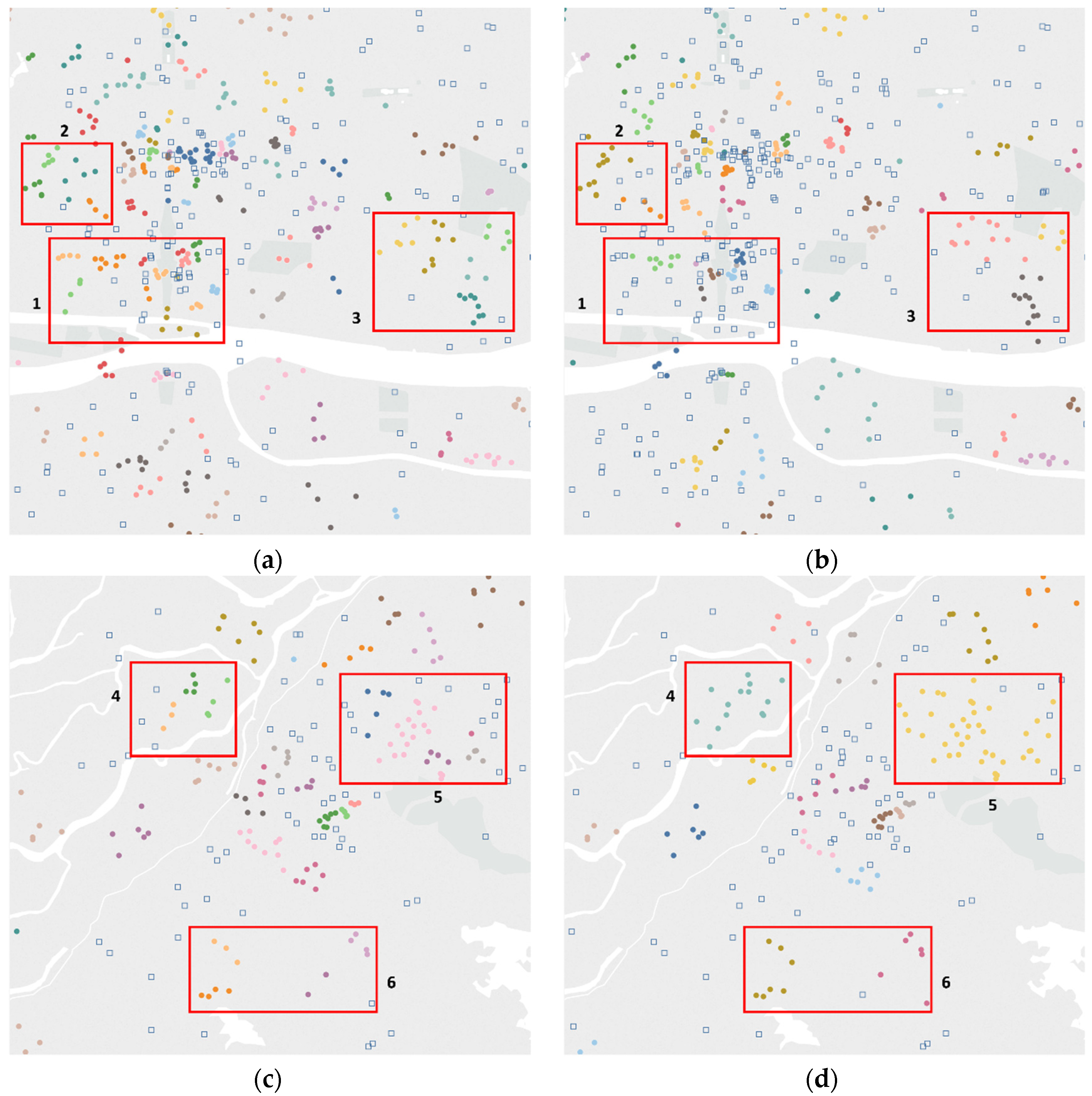
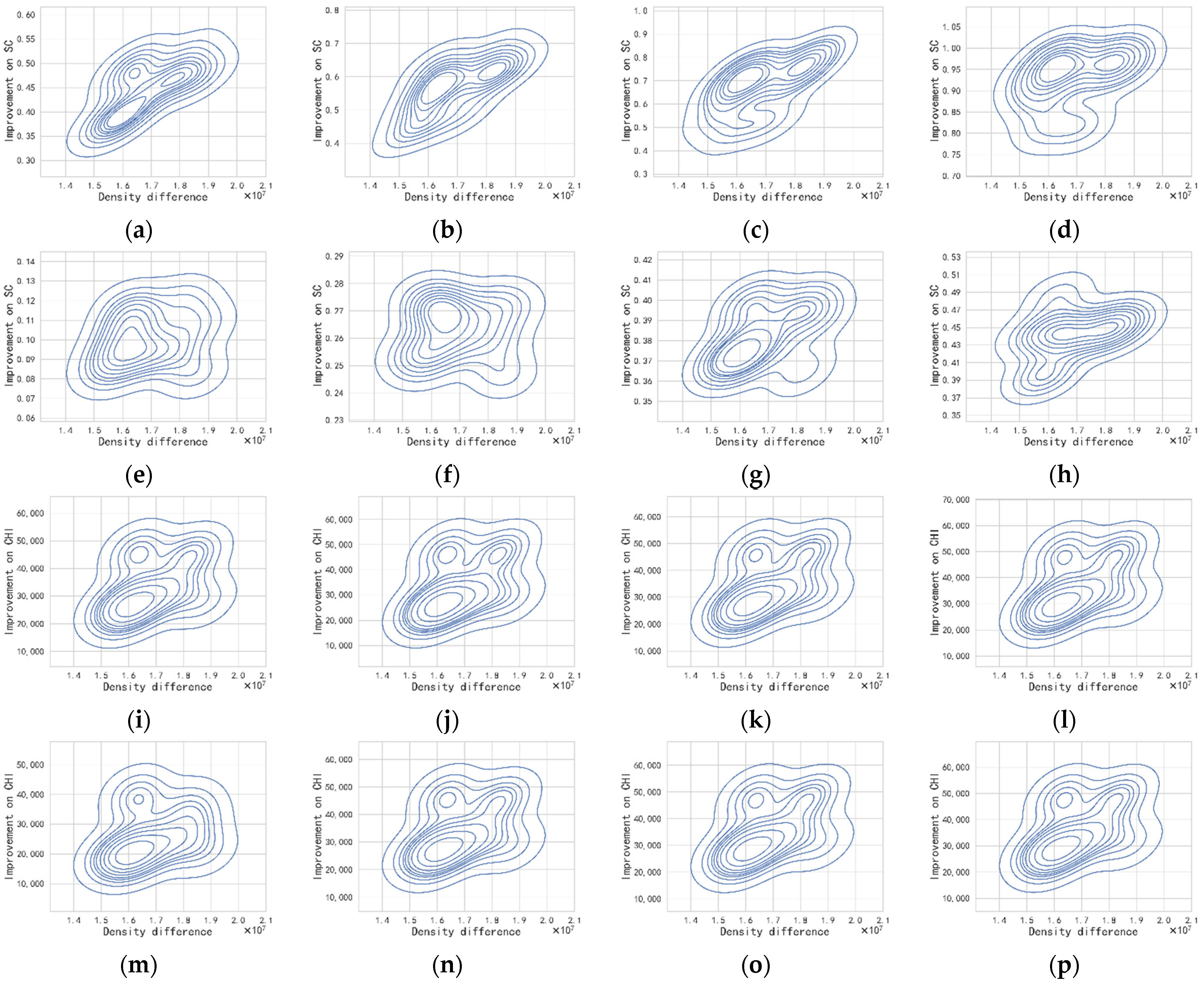
4.2. Performance Evaluation Using the Whole Datasets Based on Two Indicators

Next, we tested the methods on all the datasets, and two popular indicators were used to evaluate the performance of the results, namely the silhouette coefficient (SC) [62] and the Calinski–Harabasz index (CHI) [63]. The two indicators can describe the relationships of points in the same and different clusters, and are used for datasets with no true values. Because CHI is greatly affected by noise, we modified the calculation as $CHI(P)=CHI{(CP)}^{ratio(CP)}$, where $CP$ refers to the clustered points without noise, $CHI(CP)$ is the CHI value of clustered points, and $ratio(CP)$ is the ratio of the number of $CP$ to all points $P$. The detailed evaluation results of different methods based on SC and CHI are shown in

Table 4. Evaluation results of the different methods on the datasets based on SC.

Silhouette Coefficient (SC)		ELV	DCP	DBSCAN				HDBSCAN
				200	400	800	1600	4	8	16	32
GBA dataset	2019/12/23	0.3	−0.01	−0.27	−0.12	−0.07	−0.07	0.18	0.04	−0.06	−0.1
	2019/12/24	0.29	−0.04	−0.22	−0.11	−0.1	−0.09	0.16	0.04	−0.05	−0.12
	2019/12/25	0.31	−0.03	−0.19	−0.1	−0.14	−0.07	0.18	0.04	−0.05	−0.09
	2019/12/26	0.29	−0.04	−0.24	−0.12	−0.08	−0.07	0.18	0.04	−0.06	−0.12
	2019/12/27	0.31	−0.05	−0.29	−0.13	−0.07	−0.06	0.19	0.03	−0.07	−0.1
	2019/12/28	0.31	−0.06	−0.2	−0.05	−0.12	−0.09	0.2	0.05	−0.05	−0.08
	2019/12/29	0.33	−0.02	−0.16	−0.06	−0.12	−0.11	0.19	0.09	−0.03	−0.08
	First week	0.41	\	−0.04	−0.22	−0.33	−0.55	0.31	0.16	0.04	−0.03
	Average value of all weeks	0.4	\	−0.06	−0.18	−0.3	−0.54	0.3	0.14	0.02	−0.04
	Whole dataset	0.42	\	−0.34	−0.53	−0.66	−0.63	0.36	0.29	0.19	0.09
Shanghai dataset		0.59	\	−0.01	−0.33	−0.21	0.19	0.51	0.35	0.19	0.06
Beijing dataset		0.55	\	−0.24	−0.32	−0.14	0.03	0.48	0.33	0.18	0.06

and

Table 5. Evaluation results of the different methods on the datasets based on CHI.

Calinski–Harabasz Index (CHI)		ELV	DCP	DBSCAN				HDBSCAN
				200	400	800	1600	4	8	16	32
GBA dataset	2019/12/23	4728	229	218	433	715	1238	1172	462	293	182
	2019/12/24	4259	160	363	692	891	1658	1319	640	323	221
	2019/12/25	5894	246	451	995	1055	1467	1309	500	373	261
	2019/12/26	5635	199	282	592	813	1202	1217	518	282	146
	2019/12/27	5236	148	180	452	703	1110	1376	507	212	194
	2019/12/28	5029	158	413	999	789	1146	1248	494	251	288
	2019/12/29	5166	203	644	897	731	1157	1303	728	367	255
	First week	51,689	\	3713	2563	2636	267	10,127	3394	1484	931
	Average value of all weeks	38,210	\	3406	3212	2297	247	11,167	3085	1242	832
	Whole dataset	354,652	\	936	430	82	70	100,043	22,395	5553	2151
Shanghai dataset		47,865	\	917	535	436	484	26,206	6220	2229	916
Beijing dataset		19,526	\	312	455	579	457	11,817	5274	1707	839

. It was noted that there were no values of DPC on datasets spanning more than one day because we failed to cluster the datasets by DPC. The reason for this was that DPC uses the distances between all points and records them, which means it requires a large storage space. The number of records of one day’s data was about 15,000, and the data of a week may have been about seven times this. Correspondingly, the distances between all points needed about 49 times the storage space of one day’s data.

According to the two tables, our proposed framework showed the best performance and obtained the max values on all datasets and indicators. The SC values of ELV on the seven days were about 0.30, and those on one week were about 0.40, but the value on the whole dataset was still 0.42 with no significant improvement. The reason for this was that one day’s data was sparse and was not able to record complete human activities, and the data of one week already recorded human activities on working and rest days. The human activities described by the whole dataset may have been similar to one week, so the SC values were close. The SC values of DPC, DBSCAN 800, and 1600 were close and a little smaller than 0, which was consistent with the results shown in Figure 9. However, the CHI values of DPC, DBSCAN 800, and 1600 were very different. According to Table 3 and Figure 9, the differences between the two indicators were mainly due to the noise ratio. DPC showed similar visual results with DBSCAN 800 and 1600 with several similar large clusters, but DPC ignored the small clusters, and the noise ratio was larger. The close values of noise ratio of DPC, HDBSCAN 16 and 32 also led to similar performances on SC and CHI. The SC values of ELV on the Shanghai and Beijing datasets were 0.59 and 0.55, which were much larger than those on the GBA dataset because the GBA dataset covering 11 cities was much more complex than the Shanghai and Beijing datasets. The complexity can also be proved by Figure 1, where the GBA dataset covered much larger areas and the density differences were more significant than the other two datasets. For the same dataset, the CHI values of ELV reached dozens of times those of the other methods. The CHI value of HDBSCAN 4 was second only to ELV, but the gap was still large. Additionally, ELV obtained the largest CHI value on the whole dataset, but DBSCAN with different parameters showed even worse on the whole dataset compared with those on other datasets. It can also be seen that DBSCAN extracted small clusters with lots of noise points or only several large clusters in Figure 9. The performance in Figure 9 and Table 4 and Table 5 reflected the weakness of DBSCAN that it cannot adapt to datasets with varying densities. Combining the SC and CHI values, the improvement of ELV compared with the other methods on the GBA dataset was more significant than that on the Shanghai and Beijing datasets. This reflected the fact that ELV was more suitable for large-scale datasets than the other methods.

We also described the performances of the methods evaluated on different weeks, which are shown in Figure 12. The SC value of ELV was very stable on all weeks and larger than those of the other methods. HDBSCAN with different parameters also showed stable performances, and the SC values decreased with the increase in the parameter. DBSCAN showed the worst performance on all weeks, and the values could not remain stable. The performances of DBSCAN tested on some weeks, such as the week from 2020-01-20 to 2020-01-26, were better than those on other weeks. The reason for this may have been that the number of records on the weeks with better performance was small. The performances evaluated by CHI showed some differences, namely that ELV decreased firstly, reached the trough, and then increased. This situation may have been caused by the number of records in a week. CHI values may be influenced by data volume, and a large data volume can also better describe human activities.

Then, the influence of density difference on the clustering results was analyzed. To define density difference, we calculated the mean distances of the nearest $k$ points for each point, $mdi{s}_k\left(p_i\right)$, as follows:

$$mdi{s}_k\left(p_i\right)=\frac{{\displaystyle \sum _{l=1}^{k}di{s}_l\left(p_i\right)}}{k}$$

(12)

Then, the density difference of a point, $diff\left(p_i\right)$, was defined as the mean value of the differences between the mean distances of the point and those of other points:

$$diff\left(p_i\right)=\frac{{\displaystyle \sum _{r=1}^{n}mdi{s}_k\left(p_r\right)-mdi{s}_k\left(p_i\right)}}{n-1}$$

(13)

Finally, the density difference of whole datasets was defined as the sum of the density differences of points, ${\displaystyle \sum _{i=1}^{n}diff\left(p_i\right)}$, which can describe the overall density difference degree of all points in the dataset. This definition mainly considers the number of points close to each point and the distances between them. The value was calculated from each individual point to the whole data. Therefore, the definition can be used to describe the density difference.

Figure 13 showed the density differences of all weeks. The density difference of the week from 2020-02-03 to 2020-02-09 was the smallest, and the weeks around that time covered the Spring Festival and the Lantern Festival, and were also influenced greatly by COVID-19. The difference in the week from 2019-12-30 to 2020-01-05 was large, due to New Year’s Day. These results reflect the fact that during the Spring Festival, people go back to their hometowns, and on New Year’s Day, they like to go out in the cities covered by the GBA dataset. The last few weeks also had large differences, because people resumed work. The relationships between density difference and the improvement of ELV compared with other methods are shown in Figure 14. Overall, the improvements increased with the increase in density differences, and even presented approximately linear relationships in some figures. The linear relationships are not obvious in Figure 14e,f, which describe the comparison with HDBSCAN 4 and 8 on SC, but are more obvious on CHI, as shown in Figure 14m,n. In conclusion, ELV showed better performances both on the larger values of indicators and higher stability.

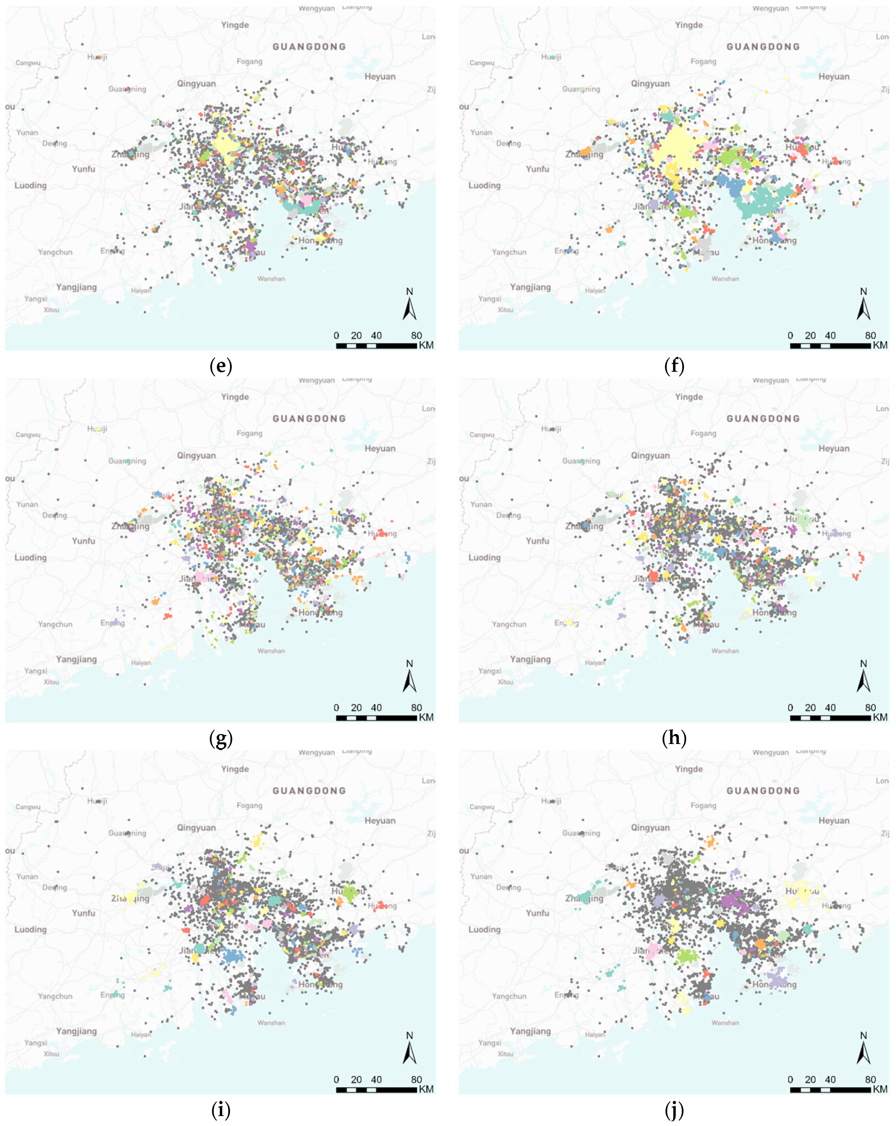
4.3. Clustering Result Analysis

In the last section, we showed the better performance of ELV than other methods, and here we further analyze the characteristics of the clustering result of ELV. The temporal characteristics of the clustering result in hours were researched, and then three features of the clusters were discussed, including how the number of points in the clusters, the area of clusters, and the density of clusters varied over the weeks studied.

The temporal characteristics of the clustering result are shown in Figure 15. The number of all points in hours firstly decreased from the hour interval 0 to 5, when most individuals slept, increased from 6 to 10, kept stable from 11 to 16, and increased finally. The value of 2019-12-25 was higher than others in many hour intervals due to Christmas Day. The values on the weekend (2019-12-28 and 29) were also larger than those on weekdays, except for those of Christmas Eve and Day. Mainly, the variation showed the life routine of individuals, such as sleep, work, and entertainment. The average number of points in each cluster can indicate the location concentration of human activities. The value varying in (b) presented the opposite case to that in (a). When most people go to bed or just stay at home late at night, the values were larger than at other times, and showed that the activity areas were concentrated. However, there were also many differences between (a) and (b), which were not simply the opposite. A wave appeared in the hour interval 1, which reflected the fact that human activities may have changed around that time. For example, some individuals may have gone home after working overtime or after leisure and entertainment. There were also two local peaks in the hour intervals 11 and 17, when individuals ended their morning and afternoon work. The values in the same interval were also different on different days. The largest value was in the hour interval 5 on 2019-12-26, and correspondingly the value in the same interval on 2019-12-25 was very low. This showed that individuals began to have a good rest after Christmas Day, and this phenomenon also appeared on the weekend. Overall, ELV was shown to be able to capture the varying characteristics of human activities over hours.

The weekly variation and distribution of different features are shown in Figure 16, which will now be analyzed. The feature k-distance refers to the average distance from a point to its nearest k points in a cluster. The average number of points in each cluster shown in (a) decreased to a min value in the week (from 2020-2-10 to 02-16) and then increased. Combining the data of three weeks shown in (f), the trough was due to the max density around 5. The densities of clusters with points less than 3 in the specific week (from 2020-2-10 to 02-16) and those with points more than 7 were smaller than those of the other two weeks. This meant individuals did not no longer concentrate in specific places, such as commercial centers, and also did not scatter in various places, such as small restaurants. They may have stayed at home due to the impact of COVID-19 in this specific week. Then, focusing on the feature of area values, it can be observed that the max values of the average area of clusters and the area occupied by each point were both in the week (from 2020-01-27 to 02-02). The reason for this may have been that individuals went out during the Spring Festival and their activity locations were dispersed, which can also be proved by the k-distance shown in (e). However, the sum area of clusters shows different weekly variations. The local peaks and troughs in (c) were similar to those in (b) and (d), but the fluctuation range was very different. For example, the max value was in the week (from 2020-02-24 to 2020-03-01). The feature sum area mainly represented the whole scope of human activities, which was influenced by the number of individuals. Therefore, different fluctuation ranges may have been because the individuals went home before the Spring Festival and went back after the impact of COVID-19 weakened. Further, we analyzed the distributions of area and k-distance in specific weeks, including the specific week (2020-01-27 to 02-02) with the max average area and k-distance, and the first and last weeks. The two features were mainly distributed in small values with an area from 0 to 0.2, and the k-distance from 0 to about 80. The specific week had the lower densities of small values and higher densities of larger values in both (g) and (h), which meant the human activities were dispersed. The first week had a higher density of small values than the last week in terms of area, and a reversed situation in terms of k-distance. This meant that the activity areas in the last week were larger than those in the first week, and showed a higher concentration.

In conclusion, our proposed framework, ELV, can capture the characteristics of human activity areas according to the above analysis.

4.4. Discussion

The strengths and weaknesses of the four algorithms compared in the above experiment are shown in

Table 6. Strengths and weaknesses of the four algorithms: our proposed algorithm (ELV), DPC, DBSCAN, and HDBSCAN.

	Strengths	Weaknesses
ELV	No manual parameter setting; Considering features of individual clusters; Fine-grained clusters generated by re-segmentation; Reduced noise points benefitting from noise recovery; Good performance on varying density spatial data	Low universality due to the special design for large-scale spatial data; Relatively slow processing efficiency;
DPC	Clear parameter selection method; Efficient high-density region extraction;	Manual parameter setting; Much slow processing efficiency on large-scale data; Neglect of low-density areas;
DBSCAN	High universality; High processing efficiency even on large-scale data; Efficient high-density region extraction with low noise ratio using large $eps$; Fine-grained clusters generated using small $eps$;	Manual parameter setting; Too many points divided into several clusters using large $eps$; Too much noise points generated using small $eps$;
HDBSCAN	High processing efficiency even on large-scale data; Only one parameter defining the min points in a cluster; Relatively good performance on varying density spatial data;	Manual parameter setting; Lots of noise points in high-density areas; Too many points divided into several clusters into low-density areas.

, mainly including parameter setting, processing efficiency, and performance on varying density data. Firstly, we focus on the aspect of parameter setting. The proposed algorithm, ELV, was specially designed for large-scale spatial data and has no manual parameter setting. The cost is the low universality, which means ELV may not be suitable for other tasks not related to spatial data. The other three algorithms are all general and can be used in many research fields. Especially, DBSCAN is such a classical algorithm, and both itself and its variants have been applied in various situations [4,23,24]. As introduced in Section 3.3, DPC has two parameters, but it provides an easy and useful method for parameter selection, but it still needs manual parameter setting for each dataset. DBSCAN has two parameters and there have been many researchers studying how to select the parameters, but manual parameter adjustment is still important for a specific task. HDBSCAN has only one parameter and the meaning of the parameter is clear, the min points in a cluster. Compared with the other three algorithms, ELV has no manual parameter setting and can be easily used in the task of human activity area extraction, but it has low universality and may not be useful in other research fields.

Processing efficiency is another important factor influencing the application of the algorithms. In the experiment, the processing efficiencies sorted from high to low were DBSCAN, HDBSCAN, ELV, and DPC. The exact processing time and memory usage in the experiment were not provided due to the codes of the algorithms were based on different underlying programming languages, which had a great influence on processing efficiency. DBSCAN and HDBSCAN use open libraries [58,59], and the processing efficiencies were much higher. We analyzed the processing efficiency according to the basic principles of the algorithms. DBSCAN and DPC both have simple processing flows, but DBSCAN got the highest efficiency and DPC was the lowest. The bad performance was due to the storage, reading, and writing of the massive distance data. For a small dataset, the size of distance data is small and DPC can process fast. However, this research focused on large-scale spatial data and DPC showed the lowest efficiency. Compared with DBSCAN and DPC, the processing flows of ELV and HDBSCAN are much more complex because they both introduce the concept of hierarchy. Additionally, ELV considers features of individual clusters when assigning no high-density points in Section 3.2.2 and adds the step of noise recovery in Section 3.2.4. The efficiency of ELV can be still high than DPC because ELV only needs a part of the distances between points. The theoretical processing efficiency is consistent with that in the experiments. Indeed, DBSCAN, HDBSCAN, and ELV all completed the extraction task in just several minutes even for the very large spatial data (the GBA dataset), but DPC suffered from a large amount of distance data.

Then, we focus on the performances of the extraction results of different algorithms. DBSCAN obtained very different clustering results with different parameters. When $eps$ was small, DBSCAN extracted fine-grained activity areas in high-density areas such as city centers, but it generated too many noise points. For low-density areas such as suburbs, there may be no cluster. With a large $eps$, DBSCAN easily extracted high-density points with very few noise points but divided too many points into several clusters. For example, a cluster may cover a city center, which made no sense for activity area extraction. The performance of DPC was very similar to DBSCAN using a large $eps$. The difference between them was that DPC only focused on high-density points and DBSCAN, using a large $eps$, still extracted clusters with low-density points. HDBSCAN showed much better performance than DBSCAN and DPC due to the concept of hierarchy. However, it still had some weaknesses that it generated many noise points to divide high-density points into different clusters and assigned some points with long distances between them into the same clusters in low-density areas. ELV improved the performance by considering features of individual clusters and recovering the noise points. As a result, ELV showed the best performance on varying density spatial data.

Additionally, the evaluation methods of clustering results need to be discussed. There are mainly three types of methods to evaluate the performance, including manual analysis, supervised evaluation, and unsupervised evaluation [21,62,63,64,65]. The most objective and effective type is supervised evaluation [21,64,65]. This can exactly describe how well the algorithms assign the points into different clusters. However, there is no truth value of human activity areas to use supervised methods. Therefore, manual analysis and unsupervised evaluation indicators were used in this research. The main statistical information of the clustering results was extracted and compared, including the number of points in clusters, the number of clusters, the areas of clusters, the ratio of noise points, and so on. The statistical data, combined with the visual analytics, helped to describe the characteristics of all the algorithms, which has been concluded previously. Then, two widely used indicators, SC and CHI [62,63], were used to evaluate the performances. Indeed, the two indicators are both based on the internal distances of points in clusters and external distances between clusters. If the sizes of clusters are very small, the internal distances become small too and make the indicators large. However, the small size of clusters may also lead to the small external distances between clusters, due to more clusters in local areas can be extracted with small sizes. The two indicators become bad with small external distances. To avoid this, some points should be considered as noise points to make the external distances large and the clustered points can obtain high indicators, but the noise points have very low values which influence the indicators of the whole data. Therefore, algorithms should trade off clustered points against noise points to get high indicators. ELV uses re-segmentation to obtain fine-grained clusters and recover noise points to reduce the ratio of noise. As a result, better performance with higher indicators can be obtained by ELV compared with other algorithms.

At last, our proposed algorithm, ELV, is compared with other related researches to discuss the innovations and advantages of this study. Many existing studies proposed or used extraction algorithms for urban hotspots based on different kinds of human activity data [15,18,38,66]. The concept of hotspots refers to the areas with a large number of points. Such areas may be famous tourist attractions, commercial centers, and so on, but they can just represent a small part of human activities. Many kinds of areas, such as restaurants and cinemas, may be ignored. This study extracts fine-grained clusters to represent human activity areas, including areas with both high- and low-densities. Therefore, a better description of human activities is obtained. There are also other studies exploring individuals’ activity areas based on clustering algorithms [4,5,26,67]. The data used in these studies for each clustering processing was an individual’s activity records. The results captured the characteristics of individuals’ activities, but are limited to the data sparse problem of an individual’s spatial data. Especially for social media data, only a small part of individuals was selected in these studies. Additionally, the clustering algorithms in the studies may show bad performances when applying them to a much more complex dataset of lots of individuals with varying densities. This study designed ELV and improved the performance for datasets with varying densities by the adaptive parameter and re-segmentation strategy. Additionally, this study focused on large-scale spatial data and used the GBA dataset covering 11 cities. Other studies only used datasets covering one city [4,18,26] and the spatial span was much smaller than that of this study. Clustering results extracted from datasets of multi-cities by our method can be helpful to discover the activity areas at the junctions of cities and better analyze the relationships between cities. Overall, ELV can better extract varying-density activity areas from whole large-scale spatial datasets compared with existing studies.

5. Conclusions

In this research, a novel framework was proposed for extracting human activity areas from large-scale spatial data with varying densities (ELV). Firstly, an automatic parameter was designed to extract and cluster high-density points, which can strengthen the practicability, especially in loops. Then, the remaining points with low densities were assigned different labels according to the spatial characteristics of the clusters with high-density points. Based on this assignment method, the framework was able to better identify noises. Further, a re-segment strategy was developed to solve the challenge of the points in a large-scale spatial dataset having larger density variations. Lastly, the additional noise points produced in the re-segment strategy were recovered to reduce noise and achieve more comprehensive area extraction. The framework was tested on three datasets, one of which covered 11 cities and had more than 1 million points. Compared with existing methods, including DBSCAN, HDBSCAN, and DPC, our proposed framework, ELV, showed the best performance according to the indicators and visual analysis. In particular, when there were many density differences, ELV was able to better adapt to the situation, and the improvements of ELV compared with the others were better.

Compared with existing studies, ELV has advantages in theoretical technologies and practical applications. There is no manual parameter setting for ELV, which can save the time of parameter adjustments and reduce the uncertainty introduced by human subjective factors. This promotes the effective use of ELV in practical application scenarios related to spatial area extraction of human activities. The assignment method distinguishes noise points by considering spatial characteristics to better describe the shape of activity areas. The re-segmentation model theoretically makes ELV adapt to varying densities and the results proved that ELV extracted fine-grained clusters in both high- and low-density areas. Some other algorithms ignored low-density areas and divided too many points into several clusters. This advantage of ELV can help analyze more detailed human activities and compare the differences between low- and high-density areas. The noise recovery is also important that it can reduce the ratio of noise points which may contain possible activity areas. Combining the assignment method and noise recovery, ELV has advantages in controlling the noise impact of human random activities with more comprehensive descriptions of activity areas compared with other studies. This characteristic of ELV is useful in the applications such as location prediction and recommendation by providing detailed and complete activity areas. The spatial span, suitable for ELV, is very large and can easily cover multi-cities, which plays a positive role in analyzing city relations. Therefore, ELV has its advantages in human activity area extraction compared with other studies.

The proposed framework is suitable for large-scale datasets due to the re-segmentation strategy. The first challenge encountered in such datasets is their varying densities, which means that many existing algorithms can only extract high-density areas or produce too much noise. The re-segmentation strategy can extract both low- and high-density clusters, and the noise can be recovered. Another challenge encountered in large-scale datasets is a large amount of computation required, which may grow exponentially with the data volume. The main budget focuses on distance calculation and query. Some algorithms, such as DPC, need to record too much distance data, and cannot work well on large-scale datasets. ELV can divide a whole clustering task into multiple subtasks, and the subtasks can continue to be divided due to the re-segmentation strategy. Therefore, distributed computing frameworks can be easily applied to ELV.

One area where this study can be enhanced is with regard to the distance measurements. This research calculated linear distances between points which is widely used in spatial clustering. Other geographical aspects can be considered, such as distances traveled by different transports between points, as well as the travel time. There are also many geographical elements, such as rivers and roads, which divide areas into different parts. Besides, semantic similarity is another good choice to measure distances between points. In this research, social media datasets were used, and the text data can be used to extract semantic information about human activities. Activity themes and emotional statuses can be extracted to describe and distinguish activity areas with different semantics. Therefore, we may intend to use the above distance measurements to enhance this study.

References

1. Shekhar, S.; Gunturi, V.; Evans, M.R.; Yang, K. Spatial big-data challenges intersecting mobility and cloud computing. In Proceedings of the Eleventh ACM International Workshop on Data Engineering for Wireless and Mobile Access, Scottsdale, AZ, USA, 20 May 2012; pp. 1–6. [Google Scholar]
2. Leszczynski, A.; Crampton, J. Introduction: Spatial big data and everyday life. Big Data Soc. 2016, 3, 2053951716661366. [Google Scholar] [CrossRef] [Green Version]
3. Khan, S.; Kannapiran, T. Indexing issues in spatial big data management. In Proceedings of the International Conference on Advances in Engineering Science Management & Technology (ICAESMT)-2019, Uttaranchal University, Dehradun, India, 14 March 2019. [Google Scholar]
4. Huang, Q. Mining online footprints to predict user’s next location. Int. J. Geogr. Inf. Sci. 2017, 31, 523–541. [Google Scholar] [CrossRef]
5. Chen, P.; Shi, W.; Zhou, X.; Liu, Z.; Fu, X. STLP-GSM: A method to predict future locations of individuals based on geotagged social media data. Int. J. Geogr. Inf. Sci. 2019, 33, 2337–2362. [Google Scholar] [CrossRef]
6. Ye, M.; Yin, P.; Lee, W.-C. Location recommendation for location-based social networks. In Proceedings of the 18th SIGSPATIAL International Conference on Advances in Geographic Information Systems, San Jose, CA, USA, 2–5 November 2010; pp. 458–461. [Google Scholar]
7. Lim, K.H.; Chan, J.; Karunasekera, S.; Leckie, C. Tour recommendation and trip planning using location-based social media: A survey. Knowl. Inf. Syst. 2019, 60, 1247–1275. [Google Scholar] [CrossRef]
8. Lian, D.; Zheng, K.; Ge, Y.; Cao, L.; Chen, E.; Xie, X. GeoMF++ scalable location recommendation via joint geographical modeling and matrix factorization. ACM Trans. Inf. Syst. 2018, 36, 33. [Google Scholar] [CrossRef]
9. Jeung, H.; Yiu, M.L.; Jensen, C.S.; Chow, C.C.-Y.; Mokbel, M.M.F. Trajectory Pattern Mining. In Computing with Spatial Trajectories; Springer: Berlin/Heidelberg, Germany, 2011; pp. 143–177. [Google Scholar] [CrossRef]
10. Cesario, E.; Comito, C.; Talia, D. A Comprehensive Validation Methodology for Trajectory Pattern Mining of GPS Data. In Proceedings of the 2016 IEEE 14th Intl Conf on Dependable, Autonomic and Secure Computing, 14th Intl Conf on Pervasive Intelligence and Computing, 2nd Intl Conf on Big Data Intelligence and Computing and Cyber Science and Technology Congress (DASC/PiCom/DataCom/CyberSciTech), Auckland, New Zealand, 13 October 2016; pp. 819–826. [Google Scholar] [CrossRef]
11. Yao, D.; Zhang, C.; Huang, J.; Bi, J. Serm: A recurrent model for next location prediction in semantic trajectories. In Proceedings of the 2017 ACM on Conference on Information and Knowledge Management, Singapore, 6–10 November 2017; pp. 2411–2414. [Google Scholar]
12. Liu, Q.; Wu, S.; Wang, L.; Tan, T. Predicting the next location: A recurrent model with spatial and temporal contexts. In Proceedings of the Thirtieth AAAI Conference on Artificial Intelligence, Phoenix, AZ, USA, 12–17 February 2016; Volume 30. [Google Scholar]
13. Chainey, S.; Tompson, L.; Uhlig, S. The utility of hotspot mapping for predicting spatial patterns of crime. Secur. J. 2008, 21, 4–28. [Google Scholar] [CrossRef]
14. Chainey, S.P. Examining the influence of cell size and bandwidth size on kernel density estimation crime hotspot maps for predicting spatial patterns of crime. Bull. Geogr. Soc. Liege 2013, 60, 7–19. [Google Scholar]
15. Yang, X.; Zhao, Z.; Lu, S. Exploring spatial-temporal patterns of urban human mobility hotspots. Sustainability 2016, 8, 674. [Google Scholar] [CrossRef] [Green Version]
16. Lawson, A.B. Hotspot detection and clustering: Ways and means. Environ. Ecol. Stat. 2010, 17, 231–245. [Google Scholar] [CrossRef]
17. Xia, Z.; Li, H.; Chen, Y.; Liao, W. Identify and delimitate urban hotspot areas using a network-based spatiotemporal field clustering method. ISPRS Int. J. Geo-Inf. 2019, 8, 344. [Google Scholar] [CrossRef] [Green Version]
18. Li, F.; Shi, W.; Zhang, H. A Two-Phase Clustering Approach for Urban Hotspot Detection with Spatiotemporal and Network Constraints. IEEE J. Sel. Top. Appl. Earth Obs. Remote Sens. 2021, 14, 3695–3705. [Google Scholar] [CrossRef]
19. Ashbrook, D.; Starner, T. Using GPS to learn significant locations and predict movement across multiple users. Pers. Ubiquitous Comput. 2003, 7, 275–286. [Google Scholar] [CrossRef]
20. Chen, Q.; Yi, H.; Hu, Y.; Xu, X.; Li, X. A New Method of Selecting K-means Initial Cluster Centers Based on Hotspot Analysis. In Proceedings of the 2018 26th International Conference on Geoinformatics, Kunming, China, 28–30 June 2018; pp. 1–6. [Google Scholar]
21. Rosenberg, A.; Hirschberg, J. V-measure: A conditional entropy-based external cluster evaluation measure. In Proceedings of the 2007 Joint Conference on Empirical Methods in Natural Language Processing and Computational Natural Language Learning (EMNLP-CoNLL), Prague, Czech Republic, 28–30 June 2007; pp. 410–420. [Google Scholar]
22. Sinaga, K.P.; Yang, M.-S. Unsupervised K-means clustering algorithm. IEEE Access 2020, 8, 80716–80727. [Google Scholar] [CrossRef]
23. Tang, J.; Liu, F.; Wang, Y.; Wang, H. Uncovering urban human mobility from large scale taxi GPS data. Phys. Stat. Mech. Appl. 2015, 438, 140–153. [Google Scholar] [CrossRef]
24. Mohammed, A.F.; Baiee, W.R. The GIS based Criminal Hotspot Analysis using DBSCAN Technique. In Materials Science and Engineering, Proceedings of the IOP Conference Series, Thi-Qar, Iraq, 15–16 July 2020; IOP Publishing: Bristol, UK, 2020; Volume 928, p. 32081. [Google Scholar]
25. Rodriguez, A.; Laio, A. Clustering by fast search and find of density peaks. Science 2014, 344, 1492–1496. [Google Scholar] [CrossRef] [Green Version]
26. Liu, X.; Huang, Q.; Gao, S. Exploring the uncertainty of activity zone detection using digital footprints with multi-scaled DBSCAN. Int. J. Geogr. Inf. Sci. 2019, 33, 1196–1223. [Google Scholar] [CrossRef]
27. Campello, R.J.G.B.; Moulavi, D.; Sander, J. Density-based clustering based on hierarchical density estimates. In Proceedings of the Pacific-Asia Conference on Knowledge Discovery and Data Mining, Gold Coast, Australia, 14–17 April 2013; pp. 160–172. [Google Scholar]
28. Jarv, P.; Tammet, T.; Tall, M. Hierarchical regions of interest. In Proceedings of the 2018 19th IEEE International Conference on Mobile Data Management (MDM), Aalborg, Denmark, 25–28 June 2018; pp. 86–95. [Google Scholar] [CrossRef]
29. Korakakis, M.; Spyrou, E.; Mylonas, P.; Perantonis, S.J. Exploiting social media information toward a context-aware recommendation system. Soc. Netw. Anal. Min. 2017, 7, 42. [Google Scholar] [CrossRef]
30. Singh, P.; Bose, S.S. Ambiguous D-means fusion clustering algorithm based on ambiguous set theory: Special application in clustering of CT scan images of COVID-19. Knowl.-Based Syst. 2021, 231, 107432. [Google Scholar] [CrossRef]
31. Jiang, Y.; Zhao, K.; Xia, K.; Xue, J.; Zhou, L.; Ding, Y.; Qian, P. A novel distributed multitask fuzzy clustering algorithm for automatic MR brain image segmentation. J. Med. Syst. 2019, 43, 118. [Google Scholar] [CrossRef]
32. Liu, Y.; Kang, C.; Gao, S.; Xiao, Y.; Tian, Y. Understanding intra-urban trip patterns from taxi trajectory data. J. Geogr. Syst. 2012, 14, 463–483. [Google Scholar] [CrossRef]
33. Yao, Z.; Zhong, Y.; Liao, Q.; Wu, J.; Liu, H.; Yang, F. Understanding human activity and urban mobility patterns from massive cellphone data: Platform design and applications. IEEE Intell. Transp. Syst. Mag. 2020, 13, 206–219. [Google Scholar] [CrossRef]
34. Jiang, S.; Ferreira, J.; Gonzalez, M.C. Activity-based human mobility patterns inferred from mobile phone data: A case study of Singapore. IEEE Trans. Big Data 2017, 3, 208–219. [Google Scholar] [CrossRef] [Green Version]
35. Zhong, C.; Batty, M.; Manley, E.; Wang, J.; Wang, Z.; Chen, F.; Schmitt, G. Variability in regularity: Mining temporal mobility patterns in London, Singapore and Beijing using smart-card data. PLoS ONE 2016, 11, e0149222. [Google Scholar]
36. Yang, F.; Ding, F.; Qu, X.; Ran, B. Estimating urban shared-bike trips with location-based social networking data. Sustainability 2019, 11, 3220. [Google Scholar] [CrossRef] [Green Version]
37. Qiao, S.; Han, N.; Huang, J.; Yue, K.; Mao, R.; Shu, H.; He, Q.; Wu, X. A Dynamic Convolutional Neural Network Based Shared-Bike Demand Forecasting Model. ACM Trans. Intell. Syst. Technol. 2021, 12, 70. [Google Scholar] [CrossRef]
38. Cai, L.; Jiang, F.; Zhou, W.; Li, K. Design and application of an attractiveness index for urban hotspots based on GPS trajectory data. IEEE Access 2018, 6, 55976–55985. [Google Scholar] [CrossRef]
39. Kang, C.; Qin, K. Understanding operation behaviors of taxicabs in cities by matrix factorization. Comput. Environ. Urban Syst. 2016, 60, 79–88. [Google Scholar] [CrossRef]
40. Zhao, S.; Zhao, P.; Cui, Y. A network centrality measure framework for analyzing urban traffic flow: A case study of Wuhan, China. Phys. Stat. Mech. Appl. 2017, 478, 143–157. [Google Scholar] [CrossRef]
41. Lv, Q.; Qiao, Y.; Ansari, N.; Liu, J.; Yang, J. Big Data Driven Hidden Markov Model Based Individual Mobility Prediction at Points of Interest. IEEE Trans. Veh. Technol. 2017, 66, 5204–5216. [Google Scholar] [CrossRef]
42. Shen, P.; Ouyang, L.; Wang, C.; Shi, Y.; Su, Y. Cluster and characteristic analysis of Shanghai metro stations based on metro card and land-use data. Geo-Spat. Inf. Sci. 2020, 23, 352–361. [Google Scholar] [CrossRef]
43. Chen, C.-F.; Huang, C.-Y. Investigating the effects of a shared bike for tourism use on the tourist experience and its consequences. Curr. Issues Tour. 2021, 24, 134–148. [Google Scholar] [CrossRef]
44. Sun, X.; Huang, Z.; Peng, X.; Chen, Y.; Liu, Y. Building a model-based personalised recommendation approach for tourist attractions from geotagged social media data. Int. J. Digit. Earth 2019, 12, 661–678. [Google Scholar] [CrossRef]
45. Cai, J.; Wei, H.; Yang, H.; Zhao, X. A novel clustering algorithm based on DPC and PSO. IEEE Access 2020, 8, 88200–88214. [Google Scholar] [CrossRef]
46. Lin, K.; Chen, H.; Xu, C.-Y.; Yan, P.; Lan, T.; Liu, Z.; Dong, C. Assessment of flash flood risk based on improved analytic hierarchy process method and integrated maximum likelihood clustering algorithm. J. Hydrol. 2020, 584, 124696. [Google Scholar] [CrossRef]
47. Lei, Y.; Zhou, Y.; Shi, J. Overlapping communities detection of social network based on hybrid C-means clustering algorithm. Sustain. Cities Soc. 2019, 47, 101436. [Google Scholar] [CrossRef]
48. Oskouei, A.G.; Hashemzadeh, M.; Asheghi, B.; Balafar, M.A. CGFFCM: Cluster-weight and Group-local Feature-weight learning in Fuzzy C-Means clustering algorithm for color image segmentation. Appl. Soft Comput. 2021, 113, 108005. [Google Scholar] [CrossRef]
49. Benabdellah, A.C.; Benghabrit, A.; Bouhaddou, I. A survey of clustering algorithms for an industrial context. Procedia Comput. Sci. 2019, 148, 291–302. [Google Scholar] [CrossRef]
50. Ahmad, A.; Khan, S.S. Survey of state-of-the-art mixed data clustering algorithms. IEEE Access 2019, 7, 31883–31902. [Google Scholar] [CrossRef]
51. Aggarwal, C.C. A survey of stream clustering algorithms. In Data Clustering; Chapman and Hall/CRC: London, UK, 2018; pp. 231–258. [Google Scholar]
52. Tabarej, M.S.; Minz, S. Rough-set based hotspot detection in spatial data. In Proceedings of the International Conference on Advances in Computing and Data Sciences, Ghaziabad, India, 12–13 April 2019; pp. 356–368. [Google Scholar]
53. Hu, Y.; Huang, H.; Chen, A.; Mao, X.-L. Weibo-COV: A Large-Scale COVID-19 Social Media Dataset from Weibo. In Proceedings of the 1st Workshop on NLP for COVID-19 (Part 2) at EMNLP 2020, Online, 20 November 2020; Association for Computational Linguistics: Cambridge, MA, USA, 2020. [Google Scholar]
54. Esri Inc. ArcGIS Pro; Esri Inc.: Redlands, CA, USA; Available online: https://www.esri.com/en-us/arcgis/products/arcgis-pro/overview (accessed on 1 June 2020).
55. Batt, S.; Grealis, T.; Harmon, O.; Tomolonis, P. Learning Tableau: A data visualization tool. J. Econ. Educ. 2020, 51, 317–328. [Google Scholar] [CrossRef]
56. McKinney, W. Data Structures for Statistical Computing in Python. In Proceedings of the 9th Python in Science Conference, Austin, TX, USA, 28 June–3 July 2010; pp. 56–61. [Google Scholar]
57. Harris, C.R.; Millman, K.J.; van der Walt, S.J.; Gommers, R.; Virtanen, P.; Cournapeau, D.; Wieser, E.; Taylor, J.; Berg, S.; Smith, N.J.; et al. Array programming with NumPy. Nature 2020, 585, 357–362. [Google Scholar] [CrossRef]
58. McInnes, L.; Healy, J.; Astels, S. hdbscan: Hierarchical density based clustering. J. Open Source Softw. 2017, 2, 205. [Google Scholar] [CrossRef]
59. Pedregosa, F.; Varoquaux, G.; Gramfort, A.; Michel, V.; Thirion, B.; Grisel, O.; Blondel, M.; Prettenhofer, P.; Weiss, R.; Dubourg, V.; et al. Scikit-learn: Machine Learning in Python. J. Mach. Learn. Res. 2011, 12, 2825–2830. [Google Scholar]
60. Hunter, J.D. Matplotlib: A 2D graphics environment. Comput. Sci. Eng. 2007, 9, 90–95. [Google Scholar] [CrossRef]
61. Waskom, M.L. Seaborn: Statistical data visualization. J. Open Source Softw. 2021, 6, 3021. [Google Scholar] [CrossRef]
62. Rousseeuw, P.J. Silhouettes: A graphical aid to the interpretation and validation of cluster analysis. J. Comput. Appl. Math. 1987, 20, 53–65. [Google Scholar] [CrossRef] [Green Version]
63. Caliński, T.; Harabasz, J. A dendrite method for cluster analysis. Commun. Stat. Methods 1974, 3, 1–27. [Google Scholar] [CrossRef]
64. Strehl, A.; Ghosh, J. Cluster ensembles—A knowledge reuse framework for combining multiple partitions. J. Mach. Learn. Res. 2002, 3, 583–617. [Google Scholar]
65. Steinley, D. Properties of the hubert-arable adjusted rand index. Psychol. Methods 2004, 9, 386. [Google Scholar] [CrossRef]
66. Yu, H.; Liu, P.; Chen, J.; Wang, H. Comparative analysis of the spatial analysis methods for hotspot identification. Accid. Anal. Prev. 2014, 66, 80–88. [Google Scholar] [CrossRef]
67. Shen, X.; Shi, W.; Chen, P.; Liu, Z.; Wang, L. Novel model for predicting individuals’ movements in dynamic regions of interest. GIScience Remote Sens. 2022, 59, 250–271. [Google Scholar] [CrossRef]
Figure 1. Heatmaps of the three datasets, namely (a) GBA dataset, (b) Shanghai dataset, and (c) Beijing dataset. The color depth indicates the density, with areas with deep color having high densities.
Ijgi 11 00397 g001
Figure 2. Statistical chart of data volume on different dates: (a) 7 days extracted from the first week in the GBA dataset; (b) the whole 12 weeks in the GBA dataset.
Ijgi 11 00397 g002
Figure 3. Workflow of ELV with four main processing steps. The parallelograms represent the raw data, processed data, and results. The rectangles refer to the three clustering steps and other steps are judgment mechanisms, shown by diamonds.
Ijgi 11 00397 g003
Figure 4. Example of the k-distance graph, which shows the distances between each point and its k nearest neighbors. An elbow point is shown in orange, and a red box describes the possible selection range of the elbow point.
Ijgi 11 00397 g004
Figure 5. Processing flow of high-density points. The parameter e p s is selected by Algorithm 1 and then high-density points can be extracted and clustered.
Ijgi 11 00397 g005
Figure 6. Assignment of remaining data. The left part shows the examples of distances between a point and clusters. The right part shows the preliminary clustering result.
Ijgi 11 00397 g006
Figure 7. Re-segmentation of one selected cluster, including the check if the data can be clustered and if the clustering result should be used to update the clustering result.
Ijgi 11 00397 g007
Figure 8. Noise recovery using the re-segmentation result of Cluster 3. There are two new clusters and lots of noise points after re-segmentation. Then, new noise points are clustered again and combined with Clusters 7 and 8 to update the clustering result.
Ijgi 11 00397 g008
Figure 9. Clustering results of different methods tested on the first day data in GBA dataset: (a) ELV, (b) DPC, (c) DBSCAN 200, (d) DBSCAN 400, (e) DBSCAN 800, (f) DBSCAN 1600, (g) HDBSCAN 4, (h) HDBSCAN 8, (i) HDBSCAN 16, and (j) HDBSCAN 32. The points colored gray were noises and points with other colors were clustered points.
Ijgi 11 00397 g009aIjgi 11 00397 g009b
Figure 10. Detailed information related to the number of points and area of clusters: (a) scatter plot of the number of points in each cluster, (b) box plot of the number of points in each cluster, (c) scatter plot of area of each cluster, (d) box plot of area of each cluster, (e) scatter plot of the area occupied by each point, and (f) box plot of the area occupied by each point.
Ijgi 11 00397 g010
Figure 11. Visual comparison of ELV and HDBSCAN in two areas with different densities based on the first day data of the GBA dataset: (a) clustering result of ELV in a high-density area, (b) clustering result of HDBSCAN 4 in a high-density area, (c) clustering result of ELV in a low-density area, and (d) clustering result of HDBSCAN 4 in a low-density area. Additionally, solid circles represent clustered points and hollow squares are noise points.
Ijgi 11 00397 g011
Figure 12. Temporal variation of the different methods evaluated by the two indicators: (a) SC and (b) CHI.
Ijgi 11 00397 g012
Figure 13. Density differences of the 12 weeks’ datasets.
Ijgi 11 00397 g013
Figure 14. Influence of density difference on the improvements of ELV compared with other methods on two indicators, namely: improvement on SC compared with (a) DBSCAN 200, (b) DBSCAN 400, (c) DBSCAN 800, (d) DBSCAN 1600, (e) HDBSCAN 4, (f) HDBSCAN 8, (g) HDBSCAN 16, and (h) HDBSCAN 32; improvement on CHI compared with (i) DBSCAN 200, (j) DBSCAN 400, (k) DBSCAN 800, (l) DBSCAN 1600, (m) HDBSCAN 4, (n) HDBSCAN 8, (o) HDBSCAN 16, and (p) HDBSCAN 32.
Ijgi 11 00397 g014
Figure 15. Temporal characteristics of the dataset of a week and the clustering result: (a) number of all points and (b) average number of points in each cluster.
Ijgi 11 00397 g015
Figure 16. Weekly variation of different features: (a) average number of points in each cluster, (b) average area of clusters, (c) sum average area of clusters, (d) area occupied by each point, and (e) average k-distance. Additionally, the distribution of (f) number of points, (g) area, and (h) k-distance in specific weeks were shown.
Ijgi 11 00397 g016aIjgi 11 00397 g016b