Identification of Metropolitan Area Boundaries Based on Comprehensive Spatial Linkages of Cities: A Case Study of the Beijing–Tianjin–Hebei Region

Abstract

As a regional management unit to solve "urban diseases,” metropolitan areas are gradually attracting widespread attention. How to objectively and accurately delineate the boundaries of a metropolitan area is the primary prerequisite for carrying out targeted studies and precisely formulating regional planning measures. However, the existing methods for delineating metropolitan area boundaries have problems, such as high data acquisition costs, subjectivity, and a single perspective of urban linkage. To address the above problems, we propose a “bottom-up” approach to metropolitan area boundary delineation based on urban comprehensive spatial linkages. We used only publicly available data to construct a directionally weighted network of urban spatial linkages, and applied community detection algorithms to delineate metropolitan area boundaries. Taking the Beijing–Tianjin–Hebei region as a case study area, the method’s validity was confirmed. The results showed the following: (1) Eight metropolitan areas were delineated within the region, with two types of metropolitan areas: “Inter-municipal” and “single-city”. (2) The overall accuracy of the delineation results reached 83.41%, which is highly consistent with their corresponding isochrone maps. (3) Most metropolitan areas were observed to have an obvious “central–peripheral” structure, with only the JingJinLang metropolitan area being a polycentric mature metropolitan area, whereas the other metropolitan areas remained in the initial stage of development, with Zhangjiakou and Chengde not yet having formed metropolitan areas. This study’s methodology highlights the basic criteria of “inter-city spatial linkage” as the foundation for boundary delineation, avoiding the inaccuracy caused by the subjective selection of boundary thresholds, and can also accurately determine the developmental stage and internal spatial structure of metropolitan areas. Our method can provide new perspectives for regional boundary delineation and spatial planning policy formulation.

1. Introduction

Over the course of two centuries of development, cities have steadily accommodated more than half of the world’s population as the territorial units in which human beings congregate. Changes such as economic globalization have led to a progressive migration of people out of the countryside and into cities, resulting in enormous urbanization on a worldwide scale and at an unprecedented rate in cities all over the world [1]. Urbanization is an inevitable stage of urban economic growth. The population and land usage of cities are rising as urbanization progresses, and although this promotes rapid socioeconomic growth, it is accompanied by a plethora of issues arising from the chaotic expansion of urban areas [2]. Unbalanced economic development [3], ‘human-land’ relationship conflict [4,5], and ecosystem degradation [6] are examples of urban diseases that indicate that rapid urbanization beyond its current capacity would stymie further development. As a result, the proper functioning of cities is critical for social and economic growth, as well as for people’s quality of life [7], yet the single model of urban development is no longer consistent with the current global trend of urbanization. The spatial structure of cities has been altered as a consequence of the drive of globalization and regional integration, and the collaborative division of labor and complementary benefits among cities have formed clusters of varied scales. As an important spatial unit for promoting regional urbanization and coordinated development, the development of metropolitan area with a central city at its core is strategic in terms of the complementary functions of cities in the region, the orderly flow of factors, the coordination of industrial division of labor, fair and balanced transportation and public service facilities, and promotion of the formation of virtuous urban development relationships, and is progressively becoming an essential component of government planning and management.

The concept of a “metropolitan area” originated in the United States, initially as a census statistical unit and then as a spatial management tool used to address urban diseases [8], and has subsequently been imitated and improved upon by other countries due to its effectiveness. In particular, Japan has focused on central and peripheral town-based commuting and logistics linkages [9]. Following its own development, China defined a metropolitan area as a combination of a major center and neighboring areas with a high proclivity for socioeconomic integration with the center [10]. To summarize the relevant definitions, a metropolitan area, as an important urban functional region and the basic unit comprising urban agglomeration [11], is characterized by a city with strong radiation-driving capacity as the core and the presence of high-intensity social, economic, and transportation spatial links with the city in the surrounding areas or urban integrated spatial units, and can break through the limitations of traditional administrative boundaries. These characteristics have been the basis of subsequent academic research on the definition of metropolitan area boundaries.

The traditional method of metropolitan area delineation research focused on the discrimination of an urban hierarchy, with the help of basic theories in geography such as the “pole–axis” theory [12], the “central–peripheral” theory [13], or the urban hinterland theory [14], and established a system of urban indicators by selecting indicators relevant to urban development; then, after qualitative evaluation, the system included cities that match the requirements within the metropolitan area [15]. Other researchers have also utilized employment data [16], demographic data [11], land prices [17], and even citizen science [18] to determine boundaries from various perspectives. The advantages of this method are that the indicators and data are easily accessible, and the delineation of boundaries is mostly achieved via urban planning, with a focus on the overall coordination of the cities within a metropolitan area; however, the disadvantage is that it could be somewhat subjective. With the inclusion of the law of gravity in urban studies, classical models such as gravity models [19,20,21], Voronoi diagrams [22], and field spread models [23] have been used to simulate the linkages between cities for boundary scoping studies, modified according to research demands. Quantitative measurement models, mainly gravity models, are more accurate and realistic in simulating inter-city interactions, emphasizing the strength of linkages between cities at the spatial scale, but neglect to analyze the internal structure of metropolitan areas. In recent years, advances in scientific and technological fields have enriched research methods and data sources. Therefore, many scholars have combined quantitative and qualitative methods to achieve metropolitan area boundary delineation using big data or remote sensing data, which has compensated for the problems of sloppy boundaries and insufficient precision of details in the delineation results of the original methods. Big data accurately represent the daily commute as a significant indicator for the definition of metropolitan areas. Li [24], Duranton [25], Bosker [26], and Wang [27] all used data related to the characterization of inter-city commuting relationships combined with GIS methods such as the threshold method to delineate the boundaries of metropolitan areas. Additionally, some scholars have also used toponym co-occurrence data [28] and POI data [29,30] to research the delineation of regional boundaries from the information and function perspectives. Even though big data may properly depict people’s living situations and delineate spatial boundaries, boundary delimitation studies still have limitations owing to objective constraints such as data collection and technology. This is why data reflecting the actual surface, such as nighttime light data [31], population spatialization data [32,33], remote sensing images [34], and geographic data [35], are increasingly being used in the research of metropolitan area boundary delimitation.

Recapping previous research, we found the following: (i) The standards and methods for delineating metropolitan area boundaries from a single perspective can no longer adequately meet the requirements of positioning metropolitan areas as spatial units for regional planning and management. (ii) In the situation of complicated linkages within a region, the existing method of delineating metropolitan area boundaries based on urban spatial linkages makes it difficult to objectively and accurately determine which metropolitan area each city clearly belongs to. With the advancement of urbanization, the structure of some metropolitan areas has gradually changed from a single-core structure to a complex structure with multiple centers [36], and the growth within the region is no longer restricted to the core city. (iii) The method of delineating metropolitan area boundaries based on the emerging big data of population activity cannot reflect the actual and static properties of metropolitan area boundaries or be applied to realistic planning. Moreover, big data are difficult to acquire in most cities or regions, while the relative actual and static flow of finance, information, transportation, and other variables can reflect a city’s radiation capacity and urban development level, which are more suitable for delineating boundaries. In conclusion, the key issue in metropolitan area boundary delineation is how to quantify the comprehensive spatial linkages generated by various levels of urban development, as well as how to achieve objective and scientific boundary delineation with a clear internal spatial structure based on complex spatial linkages.

Following the principle that “understanding urban space requires understanding flows and networks” [37], the study of urban interactions from the perspective of flow space has gradually become mainstream. With urban nodes as the unit of analysis, flow space research emphasizes the relational and connected nature of urban space [38], focusing on the analysis of network structures [39] from the perspectives of regional economies [40], tourism flows [41], population flows [42], traffic flows [43], and commuting flows [44], thus validating the flexibility and superiority of flow space for portraying urban linkages. In the meantime, with its impartiality and precision, community detection has become an innovative trend in the research of urban spatial networks [45], and it has been tentatively utilized in the evolution of urban structure [46] and the identification of spatial boundaries. For instance, Zhou [47] utilized cell phone location data to spatially delineate the internal structure of Shenzhen from the viewpoint of population migration throughout different periods. Wu [48] used a commuter taxi dataset to map national and regional economic boundaries, and Jin [49] applied community detection algorithms to map urban activity boundaries. Yin [50] used social media data to describe urban boundaries in the U.K. through a spatial interaction flow network, and Hong [51] proposed a novel approach for integrating urban roads with urban space and functional regions in Guangzhou to accomplish functional area identification. Previous research has demonstrated that integrating complex networks into geographic analysis is extremely useful for region identification and internal structure description. Consequently, in comparison to traditional approaches, the combination of complex networks and geographical analysis can achieve both quantitative measurement of comprehensive spatial linkages and depict the internal structure on the spatial scale. Additionally, the community detection algorithms can objectively categorize highly associated individuals into the same group, eliminating the problem of subjective interference in the threshold approach and ensuring accurate delineation in complex connected environments.

The primary objective of our research was to explore a “bottom-up” strategy for objectively delineating metropolitan area boundaries based on integrated linkages and precisely characterizing their internal spatial structure in the cross-disciplinary context of complex networks and geography. We designed a methodology for metropolitan area delineation based on public data. This research abstracts the comprehensive spatial connections between counties into complex urban spatial network of “nodes–edges” with the help of the improved gravity model, applies community detection algorithms to the delineation of metropolitan area boundaries, and identifies the node hierarchy of each county in the network with centrality measurements to comprehensively and objectively identify the boundaries and internal spatial patterns of each metropolitan area in the Beijing–Tianjin–Hebei region. Our main research topics herein were:

(1)

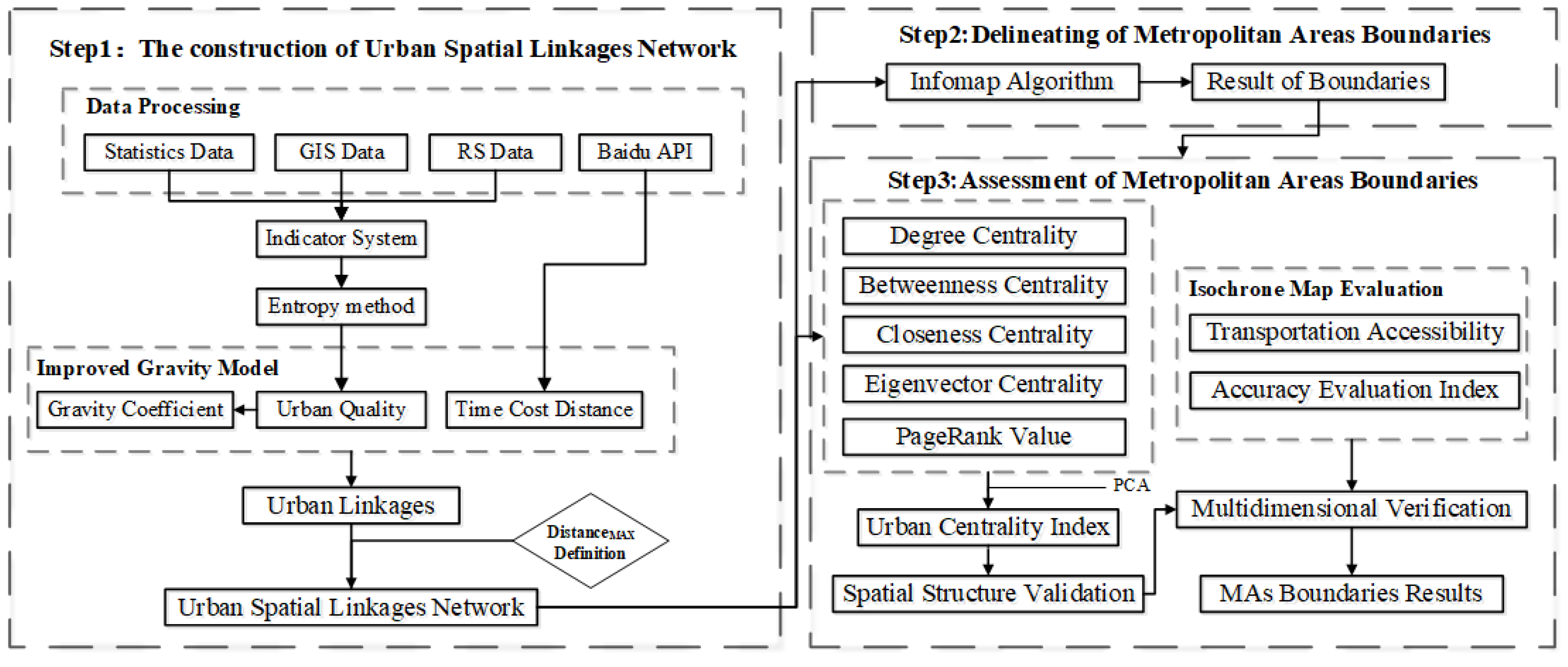
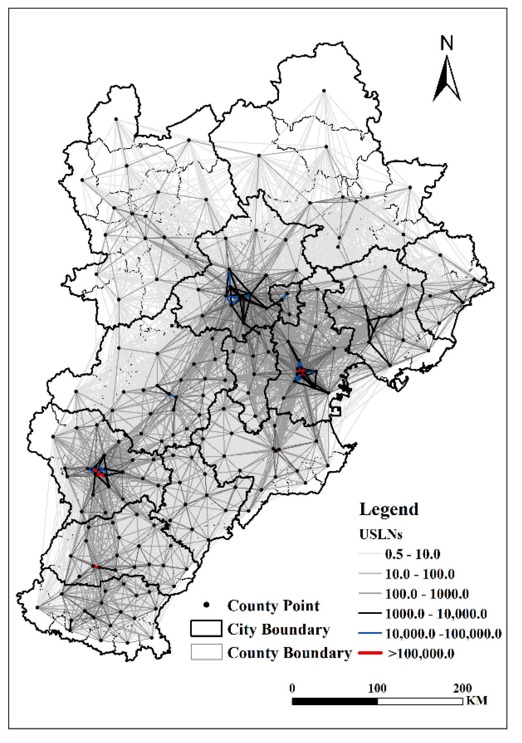
Construction of urban spatial linkage networks (USLNs). Based on the actual state of comprehensive urban development in each district and county in the study area, we measure inter-city linkages and construct an urban spatial connection network.

(2)

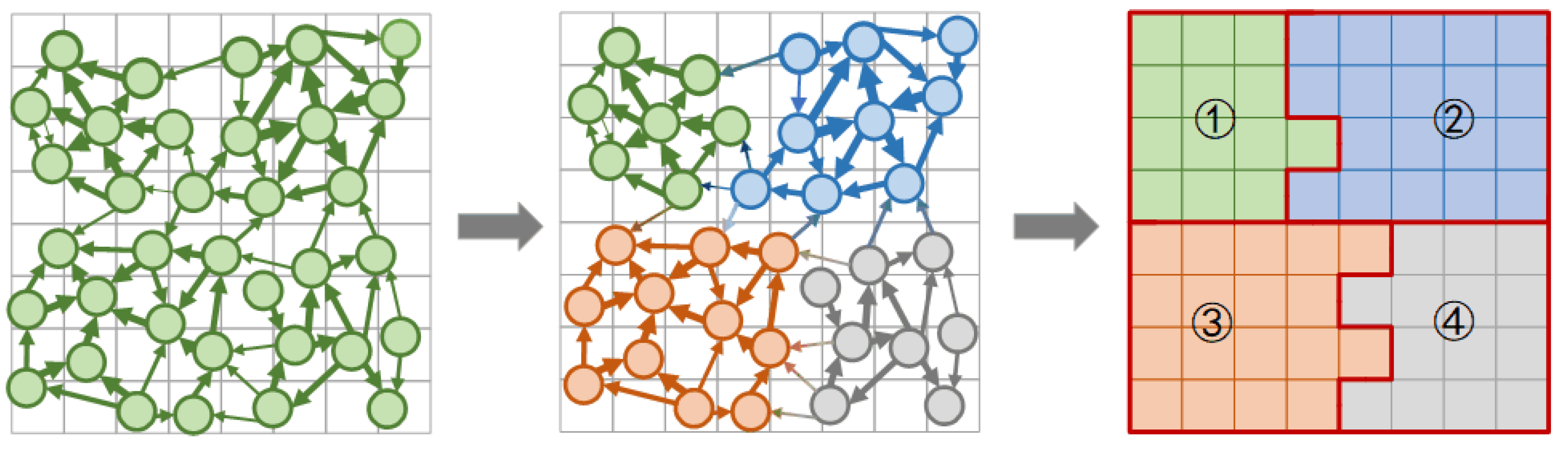
Metropolitan area boundary delineation. We delineate urban spatial linkage networks into multiple clusters and map them to geospatial units using community detection algorithms.

(3)

Assessment of delineated results. We conduct qualitative and quantitative assessment of the reliability of the boundary delineation results in terms of spatial structure rationality and isochrone map overlay analysis and then appraise the development status of each metropolitan area.

2. Materials and Methods

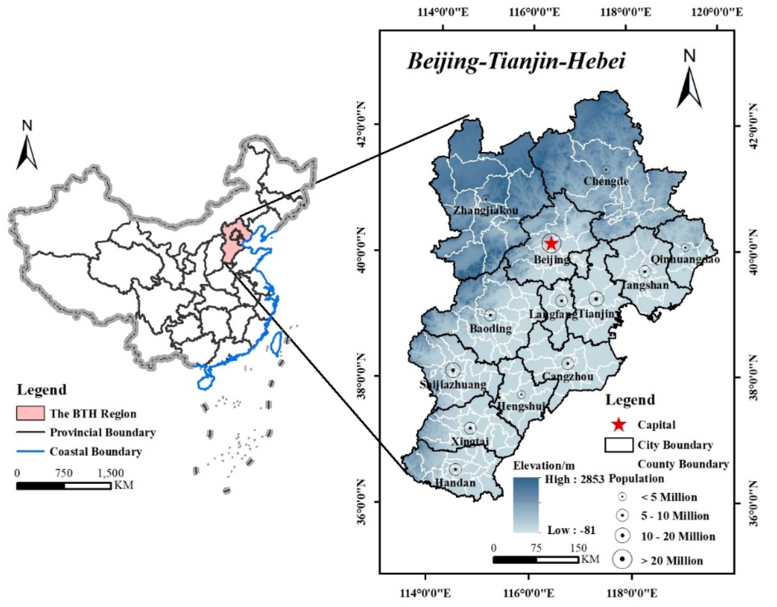
2.1. Study Area

The Beijing–Tianjin–Hebei region (36°01′42°37′ N, 113°04′119°53′ E) is located in the North China Plain, bordering the Bohai Sea in the east, with overall topography of high in the northwest and low in the southeast, including Beijing, Tianjin, two municipalities, and 11 prefecture-level cities in Hebei Province (Figure 1). It has a total population of 113.08 million (2019) and a total area of 218,000 km², with a total of 200 districts and counties in the region. The Beijing–Tianjin–Hebei region’s physiographic condition has led to the formation of four major zones: The Eastern Coastal Economic Development Zone, the Central Core Function Zone, the Northwestern Ecological Containment Zone, and the Southern Functional Expansion Zone. With the capital Beijing as the core city, Tianjin, Shijiazhuang, Tangshan, Baoding, and Handan as regional center cities, and Langfang, Cangzhou, Hengshui, Xingtai, Qinhuangdao, Zhangjiakou, and Chengde as node cities, the regional development pattern of “one core, two cities, three axes, four districts, and multiple nodes” has been formed to enhance the comprehensive carrying capacity and service quality of the city and to promote the aggregation of industries and the population.

In 2019, the GDP of the Beijing–Tianjin–Hebei region was approximately CNY 8.5 trillion, accounting for 8.62% of the national GDP, making it the third-largest economic growth pole in China, in addition to the Yangtze River Delta and the Guangdong–Hong Kong–Macao Greater Bay Area. The Beijing–Tianjin–Hebei region has experienced rapid urbanization, which has also brought about the phenomenon of imbalanced development within the region [52]. As the largest economic agglomeration in the north, the Beijing–Tianjin–Hebei region has achieved preliminary successes in terms of coordinated development, but the overall level is still lacking. High population density has caused conflicts between people and land, unequal allocation of public resources, polarization of urban development, and other regional synergy challenges. Beijing’s special status as the Chinese political and cultural center has had a particularly pronounced “siphoning effect” on capital, talent, and other development resources, but the trickle-down effect on neighboring cities has yet to be well demonstrated, and the uneven industrial structure of the three regions has resulted in Beijing and Tianjin, accounting for more than half of the region’s GDP output. The Beijing–Tianjin–Hebei Blue Book, published in March 2014, concluded that the Beijing–Tianjin–Hebei region suffers from a high concentration of megacities, insufficient absorption capacity of small and medium-sized cities, an irrational urban system structure, and powerful administration along with a powerless market, and the aforementioned issues have led to lack of support for the region’s growth and little overall potential development, which urgently needs resolving to improve the current dilemma through regional planning policies such as the metropolitan area.

2.2. Data Sources

We constructed urban static flow spatial data and measured urban spatial linkages using the three data sources listed below:

(1)

Statistical data. We collected socioeconomic and demographic data from each district and county in the Beijing–Tianjin–Hebei region in 2019 to construct GDP, population density, and other indicators to quantitatively evaluate the level of urban economic development, with data from the Beijing Regional Statistics Yearbook, Tianjin Statistical Yearbook, and Hebei Statistical Yearbook, as well as district statistical bulletins to supplement some of the missing data.

(2)

Geographic information data. We used “Basic Geographic Country Monitoring Data” to represent the research area’s surface cover, which included forest and grass cover, buildings, roads, waterways, and other types of surface cover elements that reflect the natural properties or conditions of natural and artificial structures on the ground [53]. These data provide higher resolution than other land cover data, allowing them to more precisely reflect the real land-use situation in the study area and improve the accuracy and credibility of analysis and research.

(3)

Remote sensing data. In this study, nighttime lighting data were utilized to evaluate the regional socio-economic condition, and the CHAP dataset was used to characterize the atmospheric environment. Nighttime lighting data were sourced from the Colorado School of Mines EOG group website (https://eogdata.mines.edu/products/vnl/, accessed on 29 July 2021). The data source was version2 of the 2019 annual product. Compared to the initial version of the annual synthesis data, the version2 data can more accurately reflect the urban economy [54]. The CHAP dataset is generated from the perspective of spatial and temporal heterogeneous characteristics of atmospheric pollution, combining rich ground-based observation data, satellite remote sensing products, atmospheric reanalysis, and model simulation [55]. In our research, the air quality conditions in the Beijing–Tianjin–Hebei region were described using 1 km-scale PM2.5 data from 2019.

3. Methods

We proposed a process-oriented method (Figure 2) for delineating metropolitan area boundaries based on the strength of urban linkages by combining the spatial interaction analysis method in geosciences with the concept of complex networks to accomplish delineation. First, the quality of the urban development of each district and county in the Beijing–Tianjin–Hebei region from multiple perspectives was evaluated using the collected multi-source data, and urban spatial links were quantified by the improved gravity model, with the results being abstracted into the urban spatial linkages network of urban nodes and edges described as the origin–destination style. Second, the community detection algorithm was used to complete the division of different urban clusters and then map it to geographic space to achieve rapid boundary identification. Third, we validated the results of the boundary delineation from two aspects. On the one hand, we used transportation accessibility to define an isochrones map and evaluate the objectivity and scientificity of the metropolitan area boundary results using two methods: Qualitative superposition analysis and quantitative overlapping indicators. On the other hand, the complex network analysis method was used, based on the external boundary delineation, to construct urban centrality evaluation indexes, determine the central city and internal spatial structure of the metropolitan area, and verify the scientificity of the boundary delineation from the perspective of geographic science by combining the definition of the metropolitan area in this research.

3.1. Method for the Construction of an Urban Spatial Linkages Network

The datasets used in complex network research comprise “relational data,” while the datasets used in urban spatial pattern research involve “attribute data,” which are dissimilar and cannot be directly analyzed empirically. In the era of globalization, no one city can survive in isolation; thus, there is a constant interplay of elements between cities and regions. In order to meet their own growth goals, a city grows from a single individual, with varying degrees of connection to adjacent cities, finally forming a collection of several cities. Based on this, we considered inter-city connections as network edges, districts and counties as nodes, and comprehensive city connection strength as edge weights to build the urban spatial connection network U = (N, E, W) with directional weighted attributes (Figure 3), which served as a dataset in subsequent research.

3.1.1. Measurement of Urban Quality

Urban quality is usually characterized by single indicators such as population size and GDP. However, with the depth of urban-related research, a single or a few indicators cannot reflect the whole picture. Since metropolitan areas, as integrated geographic entities have overlooked their potential function in coordinating regional development with a single indicator, we established a comprehensive indicator system (

Table 1. Integrated urban quality evaluation indicator system.

Target Layer	Guideline Layer	Indicator Layer	Unit	Indicator Meaning	Number
Integrated urban quality	Economic capability	GDP	10,000 Yuan	Regional economic power	X1
		The percentage of the added value of the tertiary industry of GDP	%	Industrial and economic structure	X2
		per capita GDP	Yuan	Living levels of residents	X3
		NTL data averages	/	Level of economic development	X4
		General public budget revenues	10,000 Yuan	Regional financial strength	X5
		General public budget expenditure	10,000 Yuan	Regional financial strength	X6
	Population capability	Resident population	10,000 people	Population scale	X7
		Urbanization rate	%	Urban development potential	X8
		Population density	people/km2	Population growth potential	X9
	Social capability	Science and technology expenditure in the general public budget expenditure	10,000 Yuan	Technological development level	X10
		Education expenditure in the general public budget expenditure	10,000 Yuan	Educational development level	X11
		Disposable income per urban resident	Yuan	Living levels of residents	X12
		Length of road per capita	m/people	Convenience of transportation	X13
		Road network density	km/km2	Level of infrastructure	X14
		Number of health facilities per 10,000 people	Institute/10,000 people	Level of health services	X18
		Number of schools per 10,000 people	Institute/10,000 people	Level of education	X19
		Percentage of built-up area	%	Land development intensity	X16
	Environmental capability	PM2.5 concentration in the air	μg/m3	Air quality level	X17
		Ecological space area	km2	Environmental quality level	X15
		Open space area per capita	people/km2	Standard of living of the population	X20

) to describe urban quality. Following the principles of data comparability, accessibility, and completeness, while taking into account the actual development of the BTH region and drawing on the indicator systems of previous relevant studies [56,57,58,59], the indicator system was constructed by selecting 20 representative indicators from four aspects: Economic capability, population capability, social capability, and environmental capability, trying to reflect the urban ability to attract and radiate influence.

Furthermore, we used multidimensional indicators to participate in the evaluation of overall quality, but the measurement units of different indicators are not uniform. To ensure the reliability of the final evaluation results, we used the entropy weighting method in the objective weighting method to calculate the weight of each indicator in the study to eliminate the influence of dimensionality. This method can determine indicator weights depending on the extent of change of each index on the overall system, thereby avoiding the influence of human factors [60].

3.1.2. Measurement of Urban Linkages

The prominent approach for urban spatial analysis studies is the gravity model. Zipf [61] was the first scholar to apply Newton’s law of gravity to the study of urban spatial interconnections in 1942, laying the groundwork for quantitative inter-city research. However, in the study of urban interactions, the classic model must be improved to reflect reality since it does not take into account the scale of urban development, economic attributes, and influencing factors [62]. Ullman [63] proposed the theory of spatial interactions, demonstrating that interactions derived from disparities in development levels between cities are out of equilibrium and that the strength of the linkages between two cities varies depending on the overall quality. Simultaneously, rapid urbanization drives the steady improvement of road traffic network construction, and it is inappropriate to distinguish distinctions across regions based just on geographical distance. Consequently, focusing on the development characteristics of the Beijing–Tianjin–Hebei region, we modified the gravity model’s urban quality, distance, and experience constant by constructing urban quality assessment indicators with locality and introducing time distance, enabling us to more accurately describe, quantitatively, the strength of external linkages and the clustering relationships of districts and counties.

Mutual radiation attraction between cities generates the “push-pull” phenomenon that offers impetus for the flow of finance, population, and other factors within the region. Therefore, the strength of the link between the two counties is deemed to be directed, and the direction of urban flow is determined based on the magnitude of the combined quality of the cities. Furthermore, as temporal distance has been proven to adequately exhibit the diversity between urban distances [64], we quantified the distance between two places based on the time cost between each district and county government point. The shortest driving distance and time between districts and counties were crawled in bulk via the Baidu Map API interface to adjust the gravity model’s distance parameters. Since the railroad network in the Beijing–Tianjin–Hebei region does not cover all districts and counties, we solely evaluated the time distance of the road transit mode. The final improved gravity model equation is as follows:

$$F_{ij}=\frac{M_i}{M_i+M_j}\frac{M_i{M}_j}{T\ast R}$$

(1)

where $F_{ij}$ is the spatial interaction intensity of two cities $i$ and $j$; $M_i\mathrm{and}{M}_j$ refer to the comprehensive urban quality of cities $i$ and $j$; $T$ is the driving time between two cities; $R$ is the shortest road distance between two cities.

3.2. Community Detection

For delineating metropolitan area boundaries, we used the Infomap algorithm to examine the aggregation of nodes in urban spatial linkage networks. The community detection algorithm originated from graph theory, which is essentially a clustering algorithm that considers extra information about the attributes of objects and focuses on the grouping of geographically linked networks based on node interaction ability [65,66]. The community detection algorithm may divide the whole network into groups based on the strength of the spatial linkages between urban nodes and ensure that the nodes within each group are the most strongly connected. Based on this, counties in the Beijing–Tianjin–Hebei region were classified into distinct groups, with the same group being a metropolitan area, and the identification results were mapped onto geospatial entities (Figure 4).

The Infomap algorithm is based on information entropy and flows [67], and its core lies in minimizing the encoding length of random walk paths and converting community division into an information flow path encoding compression. The main idea of the Infomap algorithm is to [68]: (i) Initialize the community and regard each node as a tiny community; (ii) Randomly move the nodes, with the average coding length expectation calculated separately for the case of node and community merging, and the nodes and communities that can reduce the average coding length expectation the least are merged; (iii) Repeat the iterative steps until the change is minimized. The advantage of this algorithm is that it helps determine weight and direction in a comprehensive way, based on the assumption that “each node belongs to a community uniquely,” which has significant adaptability and robustness for real network community division, making is one of the best community detection algorithms at present [69]. The equation is as follows:

$$\mathrm{H}\left(\mathrm{Q}\right)={{\displaystyle \sum }}_{i=1}^m\frac{q_i}{q}\log \left(\frac{q_i}{q}\right)$$

(2)

$$q={{\displaystyle \sum }}_{i=1}^m{q}_i$$

(3)

$$p_i=q_i+{{\displaystyle \sum }}_{\alpha \in i}{p}_{\alpha }$$

(4)

$$H\left(P_i\right)=\frac{q_i}{p_i}\log \left(\frac{q_i}{q}\right)+{{\displaystyle \sum }}_{\alpha \in i}\frac{p_{\alpha }}{p_i}\log \left(\frac{p_{\alpha }}{p_i}\right)$$

(5)

$$\mathrm{L}\left(\mathrm{M}\right)=\mathrm{qH}\left(\mathrm{Q}\right)+{\displaystyle \sum }_1^m{p}_{i}H\left(P_i\right)$$

(6)

where $\mathrm{L}\left(\mathrm{M}\right)$ denotes the average coding length expectation of the paths along which random walk occurs within and between communities; $q$ and $p_i$ denote the probability of random walk between and within communities; $m$ denotes the number of communities; $\mathrm{H}\left(\mathrm{Q}\right)$ and $H\left(P_i\right)$ denote the entropy of the probability of random wanderings moving between and within communities. According to the nature of Hoffman coding, the shortest random walk coding length corresponds to the optimal community delineation result, i.e., low probability of inter-community transfer and high probability of intra-community transfer, so the shortest coding length result was chosen as the boundary for the final identification of metropolitan areas within the Beijing–Tianjin–Hebei region.

3.3. Validation of the Results

We validated the reliability of the metropolitan area boundary results from both internal and external perspectives. The common isochrone map method for metropolitan area delineation was applied, the overlap accuracy between the metropolitan area and the isochrone map was calculated, and the geographical distribution was qualitatively determined visually. Simultaneously, we constructed centrality indicators to identify each urban node type so as to validate the rationality of the spatial structure within each metropolitan area boundary.

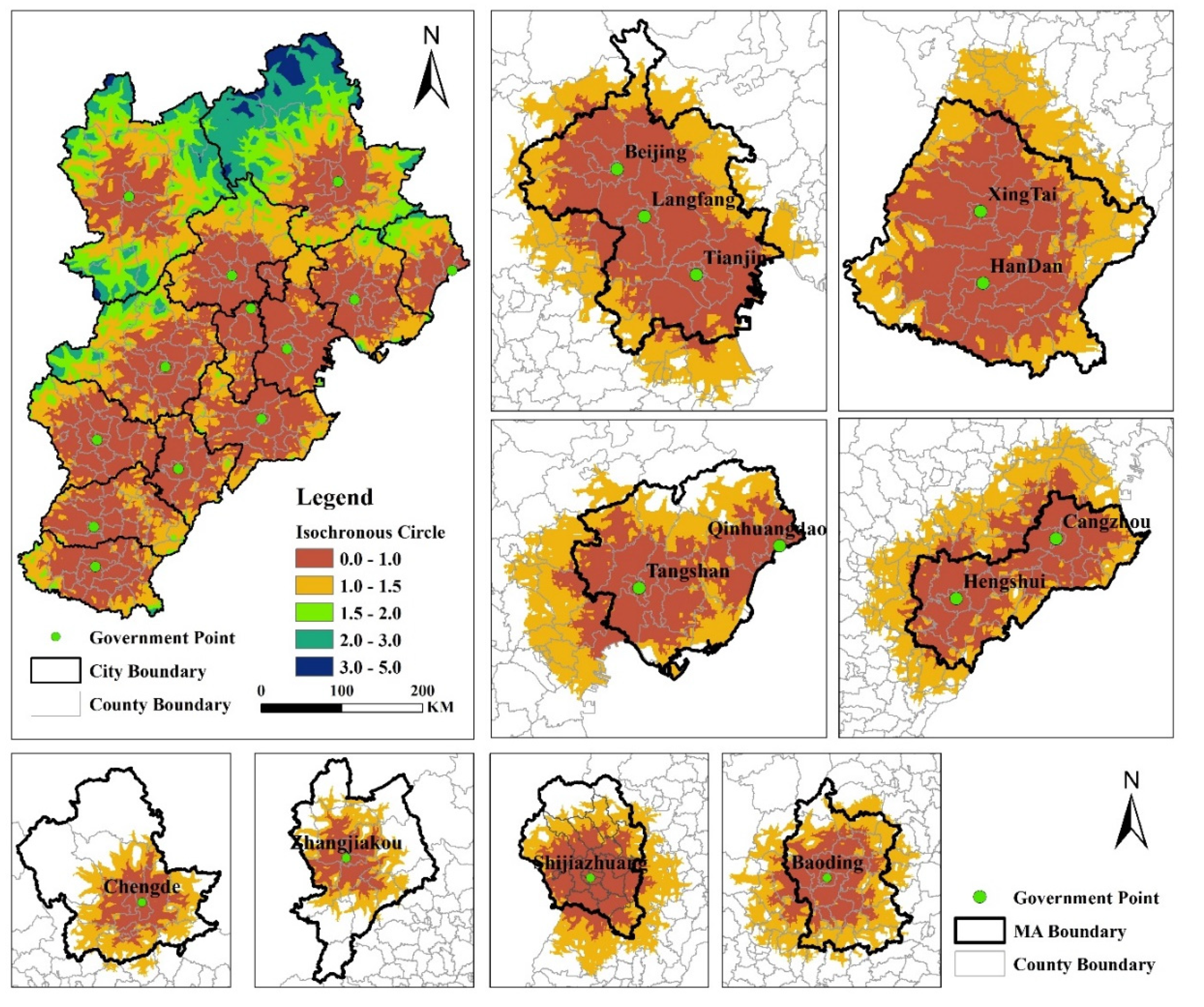
3.3.1. Isochrone Map Method

• Transportation accessibility evaluation

The isochrone map utilized the minimum cost distance method to calculate the transportation accessibility of cities in the Beijing–Tianjin–Hebei region based on the road networks by assigning values to various grades and types of roads and dividing the isochrone map to compare the accuracy of this paper in delineating metropolitan area boundaries. Combining the requirements for the population scale and traffic radiation capacity of the central city in the definition of a metropolitan area [70], Beijing and Tianjin, two municipalities directly under the central government, chose the 1.5 h isochrone map range as the final metropolitan area range, while the remaining cities chose the 1 h isochrone map range. To guarantee data comparability, the road network does not currently include railroads, where the area not covered by the road network was assigned the average speed of cycling.

Table 2. Average road speed assignment in the BTH region.

Spatial Objects	Roads				Blank Area
	National Road	Provincial Roads	County Roads	Urban Roads	Land
Speed (km/h)	90	60	60	60	10

displays the selected road categories, as well as the corresponding assigned values.

• Accuracy evaluation method

To assess the accuracy of the delineation results, we utilized the percentage of the overlap area between the delineated metropolitan area results and the corresponding isochronous overlay as an index. In particular, we used the polycentric isochrone map range for the metropolitan area of the cross-city type for computation. The formula is as follows:

$${\mathrm{Ac}}_i=\frac{M{A}_{overla{p}_i}}{I{C}_i}\times 100\%$$

(7)

where $M{A}_{overla{p}_i}$ denotes the area of each metropolitan area, $I{C}_i$ denotes the area of the corresponding isochrone map, and ${\mathrm{Ac}}_i$ denotes the accuracy rate of the result of each metropolitan area.

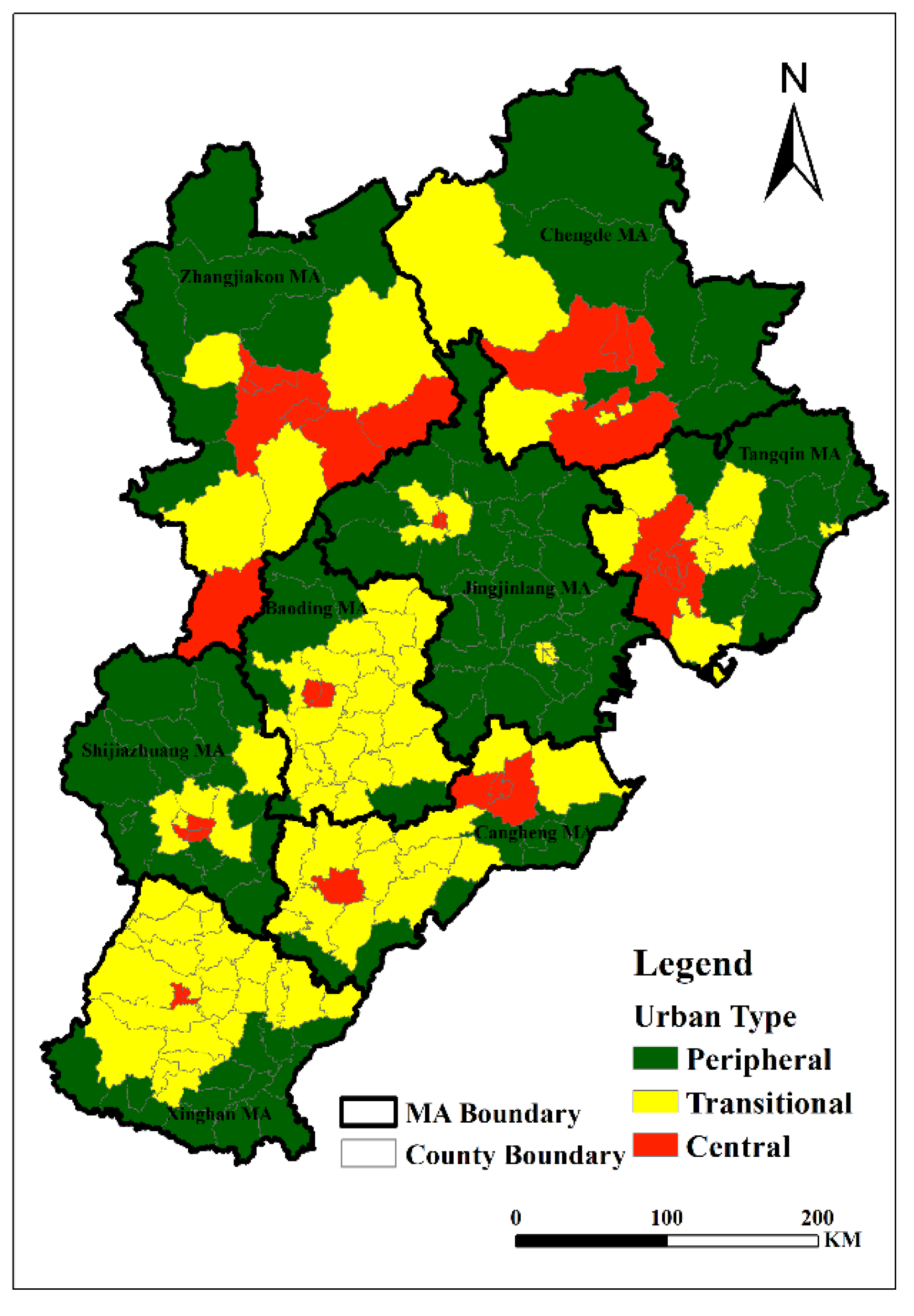
3.3.2. Rationality of the “Central-Peripheral” Structure

Cities in the metropolitan area with clear positions and different urban specializations lead to visible disparities in hierarchy across cities, thus forming a circular structure. Based on this, the rationality of the spatial organization inside the metropolitan area is also an essential part of the verification of the results. A city that interacts with more cities in the spatial network would be near the center of the metropolitan area and control the surrounding growth. We presented the centrality measure in the complex network analysis method to evaluate each city node in the network to clarify the vitality of each county in the BTH region in the overall network. Centrality is an indicator used to calculate and quantify the importance of nodes in network analysis [71], and we supplemented previous work [72,73] using principal component analysis to establish a comprehensive evaluation function of centrality and the natural breaks method to classify three types, namely, the “central type”, the “transition type”, and the “edge type” to identify the core cities and the internal spatial structure of the metropolitan area.

• Weighted Degree Centrality

Weighted degree centrality reflects how well the node is connected to other nodes and whether the node is more central in the network relative to other nodes. Weighted degree centrality in the directed graph is separated into two concepts: in-degree and out-degree. In-degree represents the size of the node that is impacted by other nodes, while out-degree reflects the node’s potential to influence other nodes. The specific formula is as follows:

$$D_i^{in}={\displaystyle \sum }_{j=1}^n{a}_{ji}{w}_{ji}$$

(8)

$$D_i^{out}={\displaystyle \sum }_{j=1}^n{a}_{ij}{w}_{ij}$$

(9)

$$D_i=D_i^{in}+D_i^{out}$$

(10)

where $n$ is the total number of city nodes; $a_{ji}$ and $a_{ij}$ denote the linkage edge with starting $j$($i$) point at the end $i$($j$) point; $w_{ji}$ and $w_{ij}$ denote the linkage weight with starting $j$($i$) point at the end $i$($j$) point; $D_i^{in}$ and $D_i^{out}$ denote the weighted in degree and weighted out degree of nodes; and $D_i$ denotes the sum of degrees.

• Closeness Centrality

The inverse of the shortest cumulative path distance from a node to all other nodes indicates closeness centrality, which reflects the proximity and accessibility of a node to other nodes in the network.

$$C{C}_i=\frac{1}{{\sum }_{j=1}^n{d}_i(i,j)}$$

(11)

where $C{C}_i$ is the closeness centrality value of each node, $n$ is the total number of city nodes, and $d_i\left(i,j\right)$ is the shortest distance between nodes $i$ and $j$.

• Betweenness Centrality

Betweenness centrality is a metric that portrays the importance of a node by the number of shortest paths passing through a node, and it can measure the control ability of a city node over the surrounding city nodes, and the higher its value, the more control it has and the more central it is in the network. The betweenness centrality formula is:

$${\mathrm{BC}}_i={\displaystyle \sum }_{j=1;k=1;j\ne k\ne i}^n\frac{N_{jk}\left(i\right)}{N_{jk}}$$

(12)

where ${\mathrm{BC}}_i$ is the intermediary centrality value of each node, $N_{jk}$ denotes the total number of shortest paths from node $j$ to $k$, and $N_{jk}\left(i\right)$ denotes the number of shortest paths between node $j$ and node $k$ through node $i.$

• Eigenvector Centrality

Eigenvector centrality judges the importance of a node based on the number of nearby nodes and their importance, emphasizing that the importance of a node is determined by both the number of neighboring nodes and the importance of its own neighboring nodes. The formula is as follows:

$${\mathrm{EC}}_i={\lambda }^{-1}{\displaystyle \sum }_{j=1}^n{a}_{ij}{x}_{ij}$$

(13)

$$\lambda e_i={\displaystyle \sum }_{j=1}^n{a}_{ij}{x}_j$$

(14)

where ${\mathrm{EC}}_i$ is the eigenvector centrality value of each node; $c$ is the proportionality constant; $A$ is the adjacency matrix, and if the node and $\left(i,j\right)$ have a connection, then $a_{ij}$ = 1, otherwise it is 0; ${\lambda }_1,{\lambda }_2,\dots \dots ,{\lambda }_n$ denotes the adjacency matrix eigenvalues, and each eigenvalue corresponds to the vector $x=\left[x_1,x_2,x_3,\dots \dots x_n\right]$.

• PageRank

On the basis of eigenvector centrality, PageRank calculates the importance of all nodes and ranks them by weight, which avoids the misjudgment of the centrality of neighboring nodes caused by the influence of high centrality nodes.

$$P{R}_i=\frac{1-q}{n}+q{\displaystyle \sum }_j\frac{P{R}_j}{L_j}$$

(15)

where $P{R}_i$ is the PageRank value of node $i$; $q$ is a constant term, generally taking the value of 0.85; $n$ is the total number of nodes; $j$ denotes the connection strength from city $i$ to city $j$; $L_j$ is the total number of all connected edges starting from node $i$, weighted by the connection strength.

• Comprehensive evaluation of urban centrality

The centrality measurement method is aimed at assessing the importance and status of city nodes in the network from many perspectives; nevertheless, the disparity in focus among the indicators leads to a lack of comparability of the results at the same level. Therefore, we used principal component analysis to eliminate the correlation between indicators, constructed a multivariate linear function to analyze and sort the importance of each node in the Beijing–Tianjin–Hebei region. The node importance comprehensive evaluation function is as follows:

$${\mathrm{Y}}_i={\beta }_1{D}_i+{\beta }_{2}C{C}_i+{\beta }_{3}B{C}_i+{\beta }_{4}E{C}_i+{\beta }_{5}P{R}_i$$

(16)

where ${\mathrm{Y}}_i$ is the comprehensive importance evaluation value of city nodes, and ${\beta }_i$ corresponds to the principal component value of each centrality measure.

4. Results

4.1. Urban Spatial Linkages Networks Construction

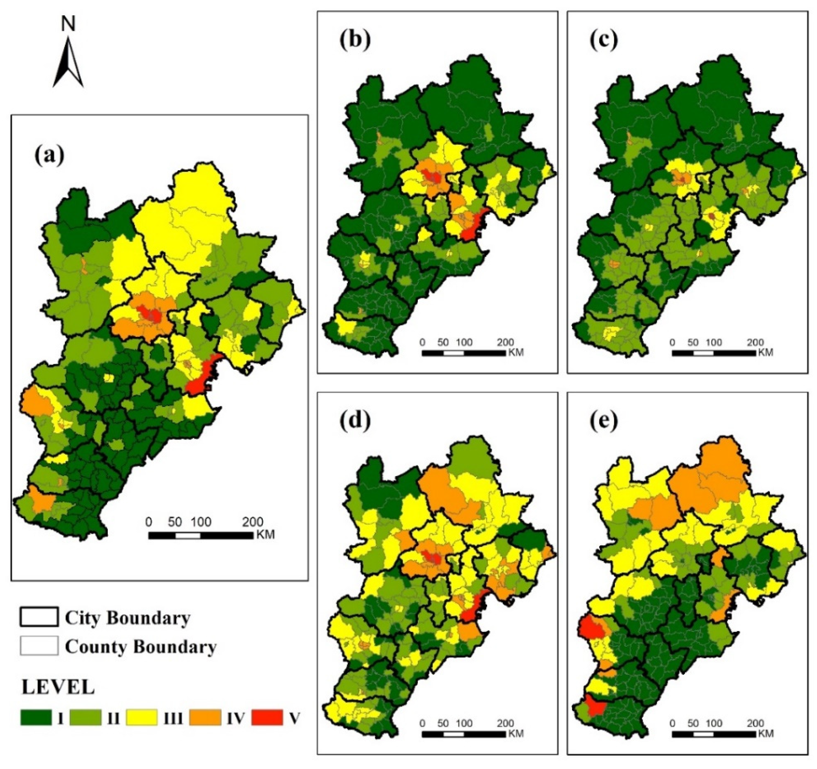
4.1.1. Urban Quality of the BTH Region

We estimated the overall urban quality of 200 districts and counties in the Beijing–Tianjin–Hebei region, as well as the urban quality associated with the four guideline tiers (Figure 5). We used the natural breaks method to classify cities into five levels of overall quality, with higher levels representing superior conditions for the city itself. As shown in Figure 5b, with the high value of the municipal area, the economic capability of various locations in the Beijing–Tianjin–Hebei region fell outward, with the total economic capability of Beijing and Tianjin being much higher than that of the cities in Hebei Province. Due to topographical factors, Zhangjiakou and Chengde, which are in the northern part of the Beijing–Tianjin–Hebei region, were hampered in their economic development, whereas Handan, Hengshui, and Xingtai, which are located far away from the radiation range of Beijing and Tianjin, were lagging in terms of economic development. In the Beijing–Tianjin–Hebei region, the population and environmental strength (Figure 5c,e) of each district and county displayed opposing spatial growth tendencies. The municipal districts of Beijing, Tianjin, and Hebei had high population capabilities. In particular, Tianjin, as the vice center of the overall region, has the highest level of population strength in the BTH region, demonstrating that it has a massive development space at present. As part of the ecologically cultured region of northwest Beijing–Tianjin–Hebei, the Chengde and Zhangjiakou’s subordinate districts and counties had restricted growth potential, while their environmental levels were superior to others. Meanwhile, as shown in Figure 5d, the mass of counties in the Beijing–Tianjin–Hebei region had low social strength, and only Beijing, Tianjin, and Tangshan had the power to empower the surrounding counties toward a more balanced growth pattern.

From a comprehensive quality perspective, the Beijing–Tianjin–Hebei area exhibited distinct polarization. Figure 5a shows that counties with lower overall urban quality were concentrated in the southeastern part of the region, with Hengshui, Cangzhou, Handan, and Xingtai having the majority of the counties with lower urban quality in the Beijing–Tianjin–Hebei region. The counties with lower urban grades were far away from the city’s municipal districts, and most prefecture-level cities lacked the radiation capacity to cover the entire municipal area; the counties with the highest urban quality were only distributed in Beijing and Tianjin, which were the four main urban areas under Beijing’s jurisdiction, namely, East and West urban areas, Chaoyang and Haidian, and Tianjin Binhai New Area.

4.1.2. Analysis of the Connection Linkage of USLNs

Because the link strength obeys the distance decay effect, the equivalent values of two counties that are far apart are very modest, even though they are linked. In the definition of a metropolitan area, we considered the actual distance and the maximum range, and finally kept node pairs with a link strengths greater than 0.5. In order to analyze the network characteristics, we divided the network into six levels, and the lowest level link was named Level VI. Figure 6 shows that the Level VI linkage network, which served as the basic linkage for the Beijing–Tianjin–Hebei region, dominated and accounted for 95% of the spatial linkage network of Beijing–Tianjin–Hebei cities when combined with Level V linkage, with only 1.4% of the high-level linkage above Level III, indicating a significant skew in the overall linkage strength.

According to the spatial distribution (Figure 7), the center part of the urban network in the Beijing–Tianjin–Hebei region was well connected, and there were no isolated nodes in the network. The connections between municipal districts and peripheral counties dominated each urban internal linkage, and the local spatial connection network was dominated by the core municipal districts to produce the central radiation phenomenon forming a more complete and denser network. Level I, II, and III linkages were mostly concentrated in Beijing, Tianjin, and Shijiazhuang, with only a minor distribution in other areas, particularly in Chengde, Zhangjiakou, and Hengshui, where Level III links were rare. At the same time, remote cities such as Zhangjiakou and Chengde, which were temporarily not highly interconnected with the main networks of Beijing, Tianjin, and Hebei and the density of the networks both inside and outside the cities was at a low level, did not interact closely with the main cities of Beijing, Tianjin, and Hebei. More than 80% of the high-level linkages were clustered in Beijing, Tianjin, Tangshan, and Shijiazhuang, allowing them to engage with other areas while retaining a high degree of contact inside the cities.

4.2. The BTH Metropolitan Area Identification Results

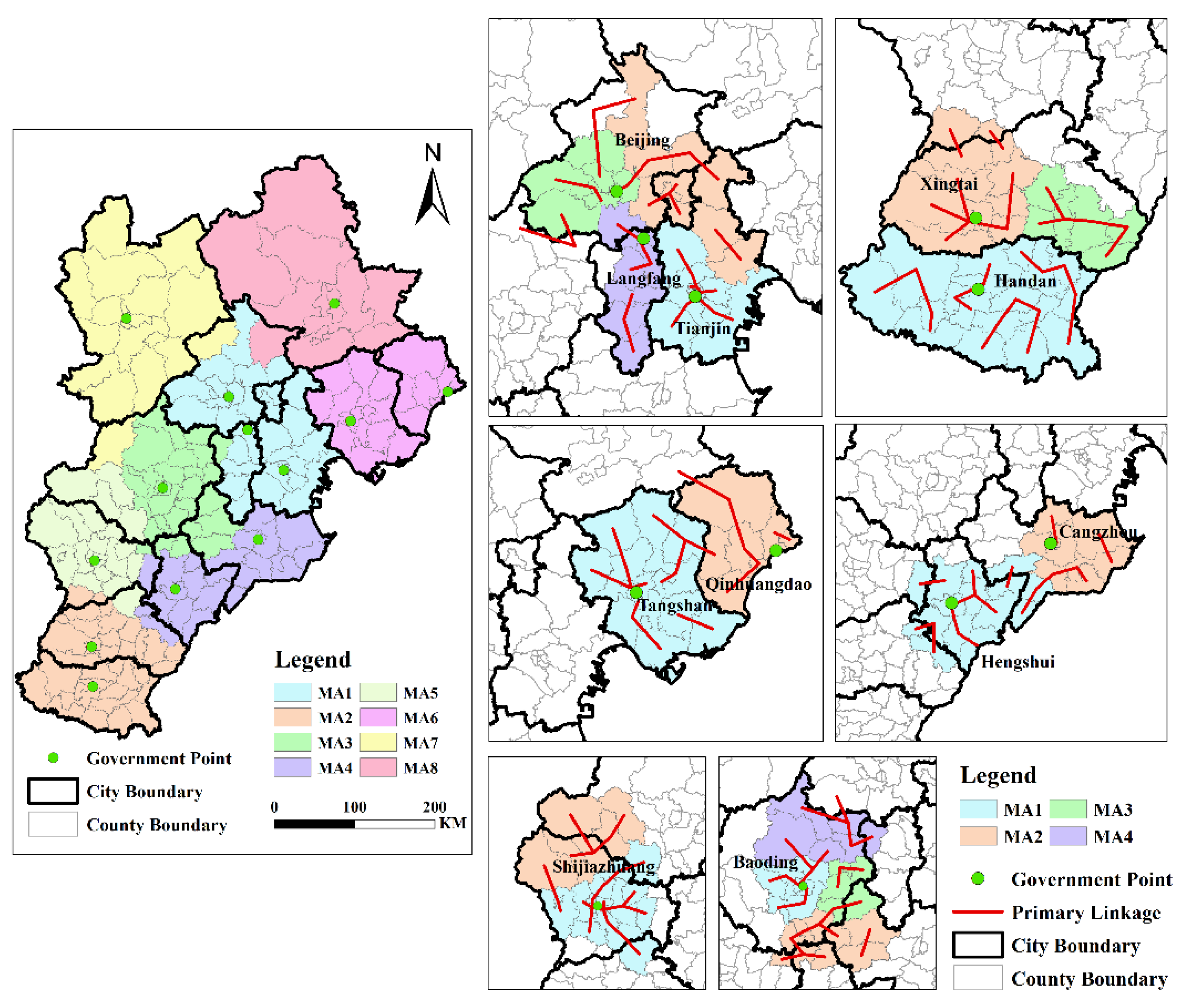
4.2.1. The Overall Visualized Identification Results

We eventually identified the boundaries of the Beijing–Tianjin–Hebei region’s metropolitan area using the Infomap algorithm, as shown in Figure 8. The Beijing–Tianjin–Hebei region was subdivided into eight metropolitan areas: Beijing–Tianjin–Langfang (JingJinLang) metropolitan area, Xingtai–Handan (XingHan) metropolitan area, Baoding (BD) metropolitan area, Cangzhou–Hengshui (CangHeng) metropolitan area, Shijiazhuang (SJZ) metropolitan area, Tangshan–Qinhuangdao (TangQin) metropolitan area, Zhangjiakou (ZJK) metropolitan area, and Chengde (CD) metropolitan area. The TangQin metropolitan area was completely contained within its administrative boundaries, with no spillover or “grabbing” by other metropolitan areas. Meanwhile, the JingJinLang and XingHan metropolitan areas retained the majority of their own districts and counties, with only a few being subdivided into other areas due to their distance from the main urban areas. Differences were observed in the administrative boundaries between the Shijiazhuang and Baoding metropolitan areas, with the Shijiazhuang metropolitan area absorbing a few southern Baoding districts and counties whilst its districts and counties adjacent to Xingtai also appeared to be absorbed by the XingHan metropolitan area. The Baoding metropolitan area, influenced by the radiation from Shijiazhuang, absorbed some of the districts and counties in Cangzhou that were not closely connected to the central city, causing the overall scope to break through the administrative division and shift toward the southeast of the BTH region. Moreover, the CangHeng metropolitan area formed a “narrow and long” development pattern, with just the city’s surrounding districts and counties constituting the main area of the metropolitan area, and was severely squeezed by the surrounding metropolitan areas.

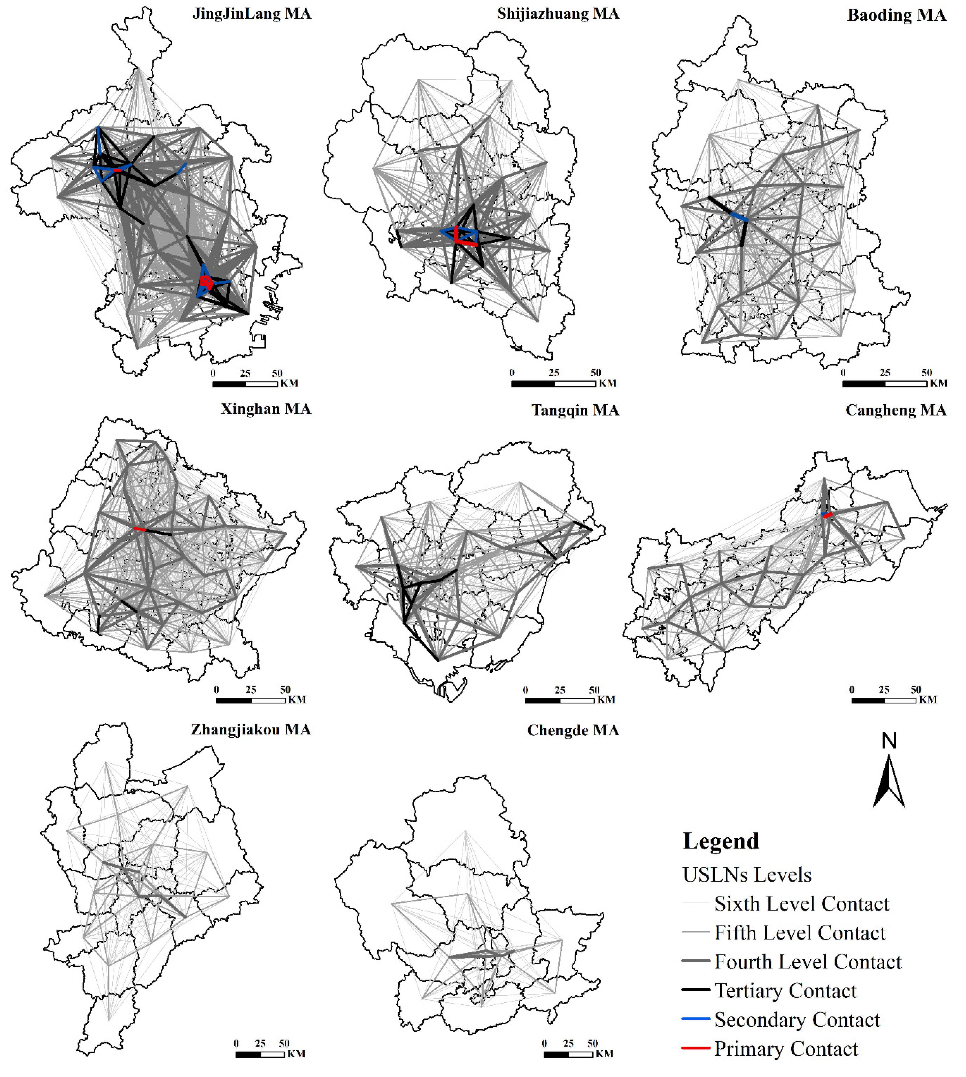
4.2.2. Linkages within Each Metropolitan Area

Following delineation, we displayed the urban spatial linkage network within each metropolitan area (Figure 9). The three metropolitan areas of JingJinLang, Shijiazhuang, and XingHan had a complete distribution of linkage levels and a relatively stable internal linkage structure, with the JingJinLang metropolitan area forming a sub-network of cities centered on Beijing and Tianjin, together forming the overall JingJinLang network. Despite having a comprehensive network of levels, the Shijiazhuang MA and XingHan MA were still dominated by low-level linkages, with networks above the tertiary level operating only inside municipal districts. The CangHeng metropolitan area, in particular, exhibited high-level network discontinuity, with Cangzhou having strong internal links but only tertiary level links with Hengshui. Zhangjiakou and Chengde, in comparison to these locations, had sparse internal networks dominated by low-level linkages, with inadequate intra-regional communication and connectivity.

As shown in Figure 10, the JingJinLang metropolitan area had the largest portion of spatial linkage flows, accounting for approximately a quarter of the total and dominating the Beijing–Tianjin–Hebei interaction; the Baoding metropolitan area came in second position overall, thanks to its placement in the midst of the Beijing–Tianjin–Hebei region and the combined radiation of Beijing and Shijiazhuang’s two core cities. The CangHeng, XingHan, and TangQin metropolitan areas, as metropolitan areas on the outskirts of the Beijing–Tianjin–Hebei region, had an equivalent number of linkages. In contrast, Zhangjiakou and Chengde rarely interacted in the region, with just a shaky connection to the JingJinLang metropolitan area.

The number of linkage flows between metropolitan areas also reflected geographical proximity. As the absolute core of the Beijing–Tianjin–Hebei region, the JingJinLang metropolitan area had links with all of the surrounding metropolitan areas, with the three metropolitan areas of TangQin, CangHeng, and Baoding accounting for around 70% of the external links of the JingJinLang metropolitan area. The TangQin and XingHan metropolitan areas had fewer external ties and only engaged, on a limited scale, with high-ranking metropolitan areas. The proportion of linkages between metropolitan areas revealed that the JingJinLang and Shijiazhuang metropolitan areas were primarily export-oriented, with a lower proportion of passive acceptance of links from other metropolitan areas. Meanwhile, the Baoding, XingHan, and CangHeng metropolitan areas struck a balance between passive acceptance and outward transmission, and the three regions of TangQin, Zhangjiakou, and Chengde were primarily passive receivers of links.

4.3. Validation of Results

4.3.1. Transportation Accessibility Evaluation

Except for a small proportion of the northern part of Chengde city and the bordering areas of Baoding and Shijiazhuang with neighboring provinces, most cities in the Beijing–Tianjin–Hebei region and their neighboring cities showed a spatial pattern of a one-hour coverage circle with the central urban area of each city as the core (Figure 11). The four major cities of Beijing, Tianjin, Tangshan, and Shijiazhuang demonstrated a faceted transportation influence radius that can intersect with nearby cities.

The results of the metropolitan area delineation were overlaid with their corresponding isochrone maps. As shown in Figure 11, the boundaries of the two were generally compatible, and there was no conflict between the metropolitan area boundaries and the extent of the isochrone maps. As the core metropolitan area of the BTH region, most of the boundaries of the JingJinLang metropolitan area were within the coverage of the 1.5 h isochrone map, and only a small part of northern Huairou was not covered. The metropolitan areas of Shijiazhuang and Baoding were wider than the 1 h isochrone map because we adhered to the characteristics of the metropolitan area and considered the convenience of regional administration; thus, the metropolitan area encompassed the whole district and county, whereas accessibility maybe not be constrained by this principle. The TangQin metropolitan area differed from the isochrone map in that its western area was not included in the TangQin metropolitan area because its overall connectivity was not stronger than the attraction of Tianjin’s main urban area to the zone. Similarly, the XingHan metropolitan area was restricted to the 1 h isochrone map. As Cangzhou and Hengshui were positioned as transportation and logistics hubs, the CangHeng metropolitan region’s transportation accessibility extended beyond the limits of the metropolitan area.

4.3.2. Accuracy Evaluation Method

Table 3. Evaluation of the accuracy of the delineation results.

Name	Overlap Area (km2)	Isochrone Map Area (km2)	AC (%)
Baoding MA	9216.87	10,836.17	85.06%
CangHeng MA	15,440.11	19,715.84	78.31%
JingJinLang MA	28,113.72	42,420.48	66.27%
Shijiazhuang MA	9429.71	11,035.74	85.45%
TangQin MA	12,385.44	14,278.10	86.74%
XingHan MA	14,861.90	15,069.56	98.62%

shows the accuracy of the delineation results, as Zhangjiakou and Chengde were entirely included in the appropriate isochrone map range and so were not included in the accuracy calculation. The overall confidence in the metropolitan area boundary delineation results was high, with the accuracy of the four metropolitan areas of XingHan, Baoding, TangQin, and Shijiazhuang exceeding 85%, while the JingJinLang metropolitan area, coinciding with the 1.5 h isochrone map had lower accuracy than the 1 h standard.

4.3.3. Spatial Structure of the Metropolitan Area

Principal component analysis was used to extract information from the centrality indicators, and a contribution rate of greater than 80% was the criterion for judgment. Finally, two principal components were obtained, and the weight of each centrality indicator was calculated according to

Table 4. Scores calculated by PCA.

Composition	Initial Eigenvalue			Component Score
	Sum	Variance Percentage	Cumulative %	D	CC	BC	EC	PR
1	3.060	61.204	61.204	0.716	0.886	0.884	0.631	0.764
2	1.078	21.551	82.755	−0.539	0.332	0.034	0.672	−0.474
3	0.404	8.074	90.829
4	0.339	6.782	97.610
5	0.119	2.390	100.000

.

The comprehensive score function was as in per Equation (17):

$${\mathrm{Y}}_i=0.6699D_i+0.6885C{C}_i+0.6417B{C}_i+0.7417E{C}_i+0.6626P{R}_i$$

(17)

We calculated the centrality score values for each district and county within the Beijing–Tianjin–Hebei region independently and came up with a mean value of 0.2496. For the convenience of narration and presentation, we calculated the number of districts and counties that were more than this mean value (Figure 12) and presented the data in the municipal form. The centrality scores of Beijing, Tianjin, Shijiazhuang, Baoding, Cangzhou, and Langfang were above the average value, demonstrating that there were districts and counties within the aforementioned cities that may serve as metropolitan area core cities. Combined with the results of city quality and boundary delineation, Beijing and Tianjin had a tiny difference in centrality scores, although Beijing had better overall urban quality than Tianjin, forming a dual-center structure within the metropolitan area; the same applied to CangHeng metropolitan area. Furthermore, due to a lack of centrality in Qinhuangdao and Handan, the TangQin and XingHan metropolitan areas were single-center structures.

To validate the spatial structure of each metropolitan area, we spatialized the centrality scores and boundaries of the metropolitan areas (Figure 13). From the metropolitan area-level structure, the JingJinLang metropolitan area is “with Beijing East and West, Chaoyang’s three districts as the core, and Tianjin’s six municipal districts as the secondary center.” Tianjin, as the sub-center, can drive the development of neighboring cities, but the two centers around more peripheral cities at present have not yet reflected its role as a central city radiation drive. The CangHeng metropolitan area had Cangzhou as its main core and Hengshui as its sub-center. The weak interconnectivity between the two centers led to a situation where there are many transitional cities and the structure needs to be optimized and improved. The monocentric metropolitan area had a clear “central-peripheral” structure and the focus of future development should be on improving its own strength and strengthening communication between the districts and counties within the metropolitan area. All the monocentric metropolitan areas featured the obvious “central-peripheral” circular structure, with peripheral cities located in geographically remote locations. To summarize the structure of the metropolitan areas in the Beijing–Tianjin–Hebei region, because of the massive gap in development levels between the central and peripheral areas, the JingJinLang metropolitan area had more peripheral counties, whereas the peripheral counties within other metropolitan areas were primarily underdeveloped due to transportation and topographical factors. Apart from the JingJinLang metropolitan area, which was in the mature stage of development, the other metropolitan areas were in the initial phases of development.

5. Discussion

5.1. Factors Influencing Metropolitan Area Boundaries

Leveraging the static flow spatial data of urban linkages, we explored the viability of using complex networks for regional administrative border demarcation investigations. The studied metropolitan areas’ boundaries approximately matched their corresponding municipal administrative boundaries. However, there are still some “disputed” districts and counties near the metropolitan areas’ borders that are subjectively perceived to be incorporated into the adjacent metropolitan area but may actually be incorporated into other metropolitan areas. For instance, some individuals in the Baoding metropolitan area decide to work in and commute to the core district of the Shijiazhuang metropolitan area, which may differ from the subjective view of most people. The main reason for this situation is that this study depicted the spatial linkages arising from actual urban growth from multiple perspectives, such as social, economic, transportation, and infrastructure construction, to achieve metropolitan area boundary delineation. It objectively reflects the radiating capacity of the central city, which delineates the boundaries of the metropolitan area from the static perspective rather than the dynamic perspective, thus leading to confusion and fragmentation in the “disputed” districts and counties. This also demonstrates how a lack of growth in the city may have a knock-on effect on the local labor market.

The network density of USLNs in the relevant areas is primarily determined by urban quality, which is one of the leading elements affecting the results of metropolitan area boundary delineation. Beijing’s political status as the capital brings its own economic welfare [74], while Tianjin’s proximity to Beijing also allows it to leverage Beijing’s development resources for its own development. Although Beijing has the highest level of internal linkage in the Beijing–Tianjin–Hebei region, its highest level of internal linkage exists only in Dongcheng District–Xicheng District, while the Yanqing and Miyun districts are less connected to the central urban area and the internal network structure is unstable. On the contrary, the six urban areas in Tianjin’s central district exhibit a high level of coordination, with the highest level of interaction intensity, obvious grouping attributes, and equally close interaction with peripheral districts and counties, hence the well-balanced overall network structure. The strength of inter-regional ties in the Beijing–Tianjin–Hebei region is transitioning from primary to intermediate, and tertiary ties across administrative boundaries are still clustered in the four major regions of development. Neighboring counties such as “Handan-Xingtai” or “Cangzhou-Hengshui” form a closer network of ties than their counterparts, demonstrating frequent travel behavior between the two regions and a trend of regional decentralization.

Because of the vast scale flow of economic and transportation elements, with a significant quantity of commuting and causing traffic among the three sites, Beijing, Tianjin, and Langfang are defined as the same metropolitan area. Due to their geographic distance from Beijing’s central city, along with topography and other natural factors that limit their development, the Yanqing and Miyun districts are not included in the JingJinLang metropolitan area, resulting in weakened interaction with the central city. As one of the core development cities, Tangshan has quite the effect in the northeast of Beijing–Tianjin–Hebei, and its geographic position with respect to Tianjin causes a “push–pull” effect with Tianjin; meanwhile, due to location restrictions, Tangshan tends to strengthen internal links and drive the development of Qinhuangdao, eventually forming a regionalized unit, which explains why the TangQin metropolitan area and administrative units coincide. Because Xingtai and Handan are located far from central cities such as Beijing and Tianjin, along with Shijiazhuang’s lack of radiation capability, it makes the interaction between Xingtai and Handan is the preferred choice to assemble a metropolitan area. The districts and counties of Baoding are separated into several collectives owing to the combined radiation of Beijing and Shijiazhuang; moreover, the effect of this metropolitan area will progressively increase in the future due to the steady growth of the Xiong’an New Area. In particular, the internal structure of Zhangjiakou and Chengde is chaotic, and urban quality, internal and external links, and centrality are all at a poor level. This is because they are designed as the ecological conservation area; thus, their own development would be restricted by various factors such as topography, resources, and industrial structure. These make them isolated in the Beijing–Tianjin–Hebei region, with neither driven by the radiation of other core cities, nor able to rely on its own development opportunities and motivations. From a synthesis perspective, Zhangjiakou and Chengde cannot be termed as a “metropolitan area” at present.

5.2. The Status of the BTH Coordinated Development

Both developed and developing countries are facing unbalanced urbanization [75], whereas metropolitan areas, as a new regional spatial unit, are rapidly attracting attention for their role in coordinated development. The coordinated development of the Beijing–Tianjin–Hebei region is still in its infancy. This study showed that there are too many high-level connections between Beijing, Tianjin, and Shijiazhuang. Thus, although the overall network appears to be dense, it is unbalanced in terms of hierarchy, especially in places such as Hengshui, which is on the fringes of the regional core city but does not benefit from the core city’s dividends. Rapid urbanization makes it difficult to ensure the harmonious development of people–land relationships. Population growth causes scarcity and uneven distribution of resources such as the environment, transportation, and public service facilities. Too many low-grade counties in the whole region reduce the number of counties that could actively receive economic radiation, making it difficult to expand the central city’s developmental achievements. Furthermore, the results of establishing sub-centers and special economic zones since the coordinated development of the BTH are not yet obvious, and in the case of the Xiong’an New Area, the overall comprehensive strength has not reached the expected level, despite the need not only to undertake relocation of industries, but also to develop high-tech independently with the core city still attracting high-tech industries to reside in, and competition emerges in multiple regions. Among the core cities, Tianjin’s Binhai New Area has grown rapidly in comparison to the Tongzhou sub-center, which still has enormous development potential. In summary, the future development of the BTH region should be based on the concept of the metropolitan area, which takes into account the development of low- and medium-grade districts and counties, while also clarifying the division of functions to break the current situation of the gradually widening development gap between two municipalities and one province.

On the basis of the results, we further delineated and added primary linkages (Figure 14). The Beijing–Tianjin–Hebei region’s metropolitan areas are still maturing, with variances in coordinated growth and different core strengths amongst cities. Small clusters within each metropolitan area are more tightly linked and impacted by their own developments, and those metropolitan areas with considerable disparities in the degree of development of internal districts and counties tend to have more small groups. There is still a need for policy direction between core urban areas and peripheral districts and counties in order to fulfill the purpose of coordinated development and increase the overall competitiveness. Under current circumstances, the spatial structure is developed and optimized in the form of urban sub-centers and satellite towns, and a polycentric structure is constructed to avoid inequities such as disproportionate regional development caused by a “single pole”.

The discrepancy in education, healthcare, and public services between districts and counties within the Beijing–Tianjin–Hebei region is too significant. Overcrowding in core city public service facilities has resulted in a steady exodus of people to cities with excellent quality of life, leading to more uneven resource allocation. The usage of metropolitan areas to “split apart” regions can be advantageous for resource optimization and equal redistribution throughout the region. Transitional cities should serve as a bridge to broaden the scope of effects and radiation and to achieve comprehensive and orderly planning in terms of industrial structure, urban functions, ecological environment, and other aspects, the central and peripheral types of districts and counties forming complementary advantages and staggered development, and gradually moving outward and forming cross-links with other metropolitan areas. Focus should be on coordination between the core and sub-core and the core and core, and engagement in growth should occur jointly in polycentric metropolitan areas, single-center metropolitan areas should emphasize core development, increase internal city node linkages, and achieve a “point-to-area” development model.

5.3. Limits and Prospects

Due to the openness and traceability of socioeconomic and geospatial data, the approach presented herein is not limited by data collection or the regional development level and can be applied to other regions. However, three main limitations of our work remain. First, as a result of the rapid urbanization process, regional management and research units will gradually be refined, so future research will not be limited to the county as the smallest research unit, and will also have the reference meaning of in-depth research on the division’s results at the town scale and even grid scales. Second, we only used isochrone map superposition analysis and internal spatial structure rationality evaluation to validate the results of the delineation of metropolitan areas. Although this is the most common method, more methods that could quantitatively describe the results are still needed. Metropolitan areas have more comprehensive and complicated boundaries as their regional units, and verification from the isochrone map alone lacks certain convincing power, necessitating the creation of an evaluation approach based on multiple perspectives. Third, with the development of the economy, transportation, and other factors, metropolitan areas are not limited to breaking through municipal administrative boundaries, and this study only considered the case of metropolitan area boundaries within the same province, not considering cross-provincial metropolitan areas. Whether this selection bias has effects on the metropolitan area boundary results needs to be further studied and explored.

6. Conclusions

As the metropolitan area is a major spatial unit of urbanization and the subject of regional cooperation and competition, objective and accurate boundaries are the basis for regional coordination studies and planning and management policy formulations. We constructed a method for delineating metropolitan area boundaries based on urban comprehensive spatial linkages and applied it to the Beijing–Tianjin–Hebei region. The results indicated that the Beijing–Tianjin–Hebei region is divided into eight metropolitan areas. Judging from the urban quality and centrality of urban nodes, there are six metropolitan areas in the Beijing–Tianjin–Hebei region and two areas where metropolitan areas have not yet been formed. Among them, the JingJinLang metropolitan area is currently a mature metropolitan area, while the rest of the metropolitan areas are in the initial stage of development. Compared to the isochrone maps and the results of previous studies, the overall accuracy of the delineated metropolitan areas reached 83.41%, and the results are credible. In summary, this approach can objectively and reliably determine the boundaries of metropolitan areas based on comprehensive inter-city linkages while eliminating the inaccuracies caused by subjective boundary threshold selection in conventional techniques.

In contrast to traditional delineation methods, our method emphasizes the core criterion of metropolitan area “urban spatial linkage” as the foundation for boundary delineation, allowing for more precise delineation and identification of metropolitan areas. Compared to identifying the region’s spatial structure from a morphological perspective, this approach highlights the region’s spatial structure during genuine development from the flow space perspective. On the one hand, by focusing on the strength of the linkages between central and neighboring cities, weaknesses in policy implementation that have long been overlooked can be identified. Therefore, our method can reflect problems with regional coordinated development and can be used by policymakers to allocate resources from the spatial perspective. On the other hand, in a situation where people are typically attracted to metropolitan areas formed by mega-cities, the approach can also be used for the general cities, which is vital to ensure the integrity of regional coordination and development. As a result, our method offers novel possibilities for delineating metropolitan area boundaries and can be used by planners and administrations.

References

1. Antrop, M. Landscape change and the urbanization process in Europe. Landsc. Urban Plan. 2004, 67, 9–26. [Google Scholar] [CrossRef]
2. Kuang, W.; Liu, J.; Dong, J.; Chi, W.; Zhang, C. The rapid and massive urban and industrial land expansions in China between 1990 and 2010: A CLUD-based analysis of their trajectories, patterns, and drivers. Landsc. Urban Plan. 2016, 145, 21–33. [Google Scholar] [CrossRef]
3. Xu, H.; Jiao, M. City size, industrial structure and urbanization quality—A case study of the Yangtze River Delta urban agglomeration in China. Land Use Policy 2021, 111, 105735. [Google Scholar] [CrossRef]
4. Zou, L.; Liu, Y.; Wang, J.; Yang, Y.; Wang, Y. Land use conflict identification and sustainable development scenario simulation on China’s southeast coast. J. Clean. Prod. 2019, 238, 117899. [Google Scholar] [CrossRef]
5. Ma, W.; Jiang, G.; Chen, Y.; Qu, Y.; Zhou, T.; Li, W. How feasible is regional integration for reconciling land use conflicts across the urban–rural interface? Evidence from Beijing–Tianjin–Hebei metropolitan region in China. Land Use Policy 2020, 92, 104433. [Google Scholar] [CrossRef]
6. McDonald, R.I.; Green, P.; Balk, D.; Fekete, B.M.; Revenga, C.; Todd, M.; Montgomery, M. Urban growth, climate change, and freshwater availability. Proc. Natl. Acad. Sci. USA 2011, 108, 6312–6317. [Google Scholar] [CrossRef] [PubMed] [Green Version]
7. Brezzi, M. Redefining “Urban”: A New Way to Measure Metropolitan Areas; OECD: Paris, France, 2012. [Google Scholar]
8. Klove, R.C. The definition of standard metropolitan areas. Econ. Geogr. 1952, 28, 95–104. [Google Scholar] [CrossRef]
9. Tan, Z. The Formation, Problems and its Countermeasure of Tokyo Megalopolis: A Lesson to Beijing. Urban Plan. Overseas 2000, 2, 8–11+43. [Google Scholar]
10. Zhou, Y. Urban Geography; The Commercial Press: Beijing, China, 1995. [Google Scholar]
11. Ning, Y. Definition of Chinese Metropolitan Areas and Large Urban Agglomerations:Role of Large Urban Agglomerations in Regional Development. Sci. Geogr. Sin. 2011, 31, 257–263. [Google Scholar] [CrossRef]
12. Gao, X.; Xu, Z.; Niu, F. Delineating the scope of urban agglomerations based upon the Pole-Axis theory. Prog. Geogr. 2015, 34, 280–289. [Google Scholar] [CrossRef]
13. Chen, S.; Huang, J. Review of range recognition research on urban agglomerations. Prog. Geogr. 2015, 34, 313–320. [Google Scholar] [CrossRef]
14. Wang, C.; Hao, Z.; Yao, S.; Ding, Q. Study on the hinterland area of center cities in urban agglomerations era—A case study of jinan. Hum. Geogr. 2012, 27, 78–82. [Google Scholar] [CrossRef]
15. Gottmann, J. Megalopolis or the Urbanization of the Northeastern Seaboard. Urban Plan. Int. 1957, 33, 189–200. [Google Scholar] [CrossRef]
16. Yu, T.; Wu, Z. Boundary analysis of the Yangtze delta megalopolis region. Resour. Environ. Yangtze Basin 2005, 14, 397–403. [Google Scholar]
17. Bode, E. Delineating metropolitan areas using land prices. J. Reg. Sci. 2010, 48, 131–163. [Google Scholar] [CrossRef]
18. Bedessem, B.; Gawrońska-Nowak, B.; Lis, P. Can citizen science increase trust in research? A case study of delineating Polish metropolitan areas. J. Contemp. Eur. Res. 2021, 17, 304–325. [Google Scholar] [CrossRef]
19. Huff, D.L.; Lutz, J.M. Change and Continuity in the Irish Urban System, 1966–1981. Urban Stud. 1995, 32, 155–174. [Google Scholar] [CrossRef]
20. Huff, D.L.; Lutz, J.M. Urban spheres influence in Ghana. J. Dev. Areas 1989, 23, 201–220. [Google Scholar]
21. Abedini, A.; Ebrahimkhani, H.; Abedini, B. Mixed Method Approach to Delineation of Functional Urban Regions: Shiraz Metropolitan Region. J. Urban Plan. Dev. 2016, 142, 04016001. [Google Scholar] [CrossRef]
22. Mu, L.; Wang, X. Population landscape: A geometric approach to studying spatial patterns of the US urban hierarchy. Int. J. Geogr. Inf. Sci. 2006, 20, 649–667. [Google Scholar] [CrossRef]
23. Liang, S. Research on the Urban Influence Domains in China. Int. J. Geogr. Inf. Sci. 2009, 23, 1527–1539. [Google Scholar] [CrossRef]
24. Li, K.; Niu, X. Delineation of the Shanghai Megacity Region of China from a Commuting Perspective: Study Based on Cell Phone Network Data in the Yangtze River Delta. J. Urban Plan. Dev. 2021, 147, 04021022. [Google Scholar] [CrossRef]
25. Duranton, G. Delineating Metropolitan Areas: Measuring Spatial Labour Market Networks through Commuting Patterns. Econ. Interfirm Netw. 2015, 127, 107–133. [Google Scholar] [CrossRef]
26. Bosker, M.; Park, J.; Roberts, M. Definition matters. Metropolitan areas and agglomeration economies in a large-developing country. J. Urban Econ. 2021, 125, 103275. [Google Scholar] [CrossRef]
27. Wang, D.; Gu, J.; Yan, L. Delimiting the Shanghai metropolitan area using mobile phone data. Acta Geogr. Sin. 2018, 73, 1896–1909. [Google Scholar]
28. Wu, J.; Feng, Z.; Zhang, X.; Xu, Y.; Peng, J. Delineating urban hinterland boundaries in the Pearl River Delta: An approach integrating toponym co-occurrence with field strength model. Cities 2020, 96, 102457. [Google Scholar] [CrossRef]
29. Lv, Y.; Zhou, L.; Yao, G.; Zheng, X. Detecting the true urban polycentric pattern of Chinese cities in morphological dimensions: A multiscale analysis based on geospatial big data. Cities 2021, 116, 103298. [Google Scholar] [CrossRef]
30. Zhen, F.; Cao, Y.; Qin, X.; Wang, B. Delineation of an urban agglomeration boundary based on Sina Weibo microblog ‘check-in’ data: A case study of the Yangtze River Delta. Cities 2017, 60, 180–191. [Google Scholar] [CrossRef]
31. Dingel, J.I.; Miscio, A.; Davis, D.R. Cities, lights, and skills in developing economies. J. Urban Econ. 2021, 125, 103174. [Google Scholar] [CrossRef]
32. He, X.; Yuan, X.; Zhang, D.; Zhang, R.; Li, M.; Zhou, C. Delineation of Urban Agglomeration Boundary Based on Multisource Big Data Fusion—A Case Study of Guangdong–Hong Kong–Macao Greater Bay Area (GBA). Remote Sens. 2021, 13, 1801. [Google Scholar] [CrossRef]
33. Moreno-Monroy, A.I.; Schiavina, M.; Veneri, P. Metropolitan areas in the world. Delineation and population trends. J. Urban Econ. 2021, 125, 103242. [Google Scholar] [CrossRef]
34. Fragkias, M.; Seto, K.C. Evolving rank-size distributions of intra-metropolitan urban clusters in South China. Comput. Environ. Urban Syst. 2009, 33, 189–199. [Google Scholar] [CrossRef]
35. Khalili, A.; Besselaar, P.; Graaf, K. Using Linked Open Geo Boundaries for Adaptive Delineation of Functional Urban Areas. In Proceedings of the ESWC 2018 Satellite Events, Heraklion, Greece, 3–7 June 2018; Revised Selected Papers. Springer: Cham, Switzerland, 2018; Volume 11155, pp. 327–341. [Google Scholar] [CrossRef]
36. Veneri, P. The identification of sub-centres in two Italian metropolitan areas: A functional approach. Cities 2013, 31, 177–185. [Google Scholar] [CrossRef] [Green Version]
37. Batty, M. The New Science of Cities; MIT Press: Cambridge, MA, USA, 2013. [Google Scholar]
38. Pflieger, G.; Rozenblat, C. Introduction. Urban Networks and Network Theory: The City as the Connector of Multiple Networks. Urban Stud. 2010, 47, 2723–2735. [Google Scholar] [CrossRef] [Green Version]
39. Jin, R.; Gong, J.; Deng, M.; Wan, Y.; Yang, X. A Framework for Spatiotemporal Analysis of Regional Economic Agglomeration Patterns. Sustainability 2018, 10, 2800. [Google Scholar] [CrossRef] [Green Version]
40. Sun, Q.; Tang, F.; Tang, Y. An economic tie network-structure analysis of urban agglomeration in the middle reaches of Changjiang River based on SNA. J. Geogr. Sci. 2015, 25, 739–755. [Google Scholar] [CrossRef] [Green Version]
41. Liu, Y.; Liao, W. Spatial Characteristics of the Tourism Flows in China: A Study Based on the Baidu Index. ISPRS Int. J. Geo-Inf. 2021, 10, 378. [Google Scholar] [CrossRef]
42. Yang, Z.; Gao, W.; Zhao, X.; Hao, C.; Xie, X. Spatiotemporal Patterns of Population Mobility and Its Determinants in Chinese Cities Based on Travel Big Data. Sustainability 2020, 12, 4012. [Google Scholar] [CrossRef]
43. Ren, M.; Xiao, Z.; Wang, J. Spatial pattern of intercity less-than-truckload logistics networks in China. Acta Geogr. Sin. 2020, 75, 820–832. [Google Scholar]
44. Sarkar, S.; Wu, H.; Levinson, D. Measuring polycentricity via network flows, spatial interaction and percolation. Urban Stud. 2020, 57, 2402–2422. [Google Scholar] [CrossRef]
45. Liu, Y.; Sui, Z.; Kang, C.; Gao, Y. Uncovering patterns of inter-urban trip and spatial interaction from social media check-in data. PLoS ONE 2014, 9, e86026. [Google Scholar] [CrossRef] [PubMed]
46. Zhang, Y.; Marshall, S.; Cao, M.; Manley, E.; Chen, H. Discovering the evolution of urban structure using smart card data: The case of London. Cities 2021, 112, 103157. [Google Scholar] [CrossRef]
47. Zhou, M.; Yue, Y.; Li, Q.; Wang, D. Portraying Temporal Dynamics of Urban Spatial Divisions with Mobile Phone Positioning Data: A Complex Network Approach. ISPRS Int. J. Geo-Inf. 2016, 5, 240. [Google Scholar] [CrossRef] [Green Version]
48. Wu, C.; Smith, D.; Wang, M. Simulating the urban spatial structure with spatial interaction: A case study of urban polycentricity under different scenarios. Comput. Environ. Urban Syst. 2021, 89, 101677. [Google Scholar] [CrossRef]
49. Jin, M.; Gong, L.; Cao, Y.; Zhang, P.; Gong, Y.; Liu, Y. Identifying borders of activity spaces and quantifying border effects on intra-urban travel through spatial interaction network. Comput. Environ. Urban Syst. 2021, 87, 101625. [Google Scholar] [CrossRef]
50. Yin, J.; Soliman, A.; Yin, D.; Wang, S. Depicting urban boundaries from a mobility network of spatial interactions: A case study of Great Britain with geo-located Twitter data. Int. J. Geogr. Inf. Sci. 2017, 31, 1293–1313. [Google Scholar] [CrossRef] [Green Version]
51. Hong, Y.; Yao, Y. Hierarchical community detection and functional area identification with OSM roads and complex graph theory. Int. J. Geogr. Inf. Sci. 2019, 33, 1569–1587. [Google Scholar] [CrossRef]
52. Hu, Y.; Peng, J.; Liu, Y.; Du, Y.; Li, H.; Wu, J. Mapping Development Pattern in Beijing-Tianjin-Hebei Urban Agglomeration Using DMSP/OLS Nighttime Light Data. Remote Sens. 2017, 9, 760. [Google Scholar] [CrossRef] [Green Version]
53. Mao, W.; Zhao, H.; Gao, W.; Tu, H.; Xu, Y. Research on Quality Control Method of Land Cover Classification Data Oriented to National Geographic Condition Monitoring. ISPRS Ann. Photogramm. Remote Sens. Spat. Inf. Sci. 2021, 3, 265–269. [Google Scholar] [CrossRef]
54. Elvidge, C.D.; Zhizhin, M.; Ghosh, T.; Hsu, F.-C.; Taneja, J. Annual Time Series of Global VIIRS Nighttime Lights Derived from Monthly Averages: 2012 to 2019. Remote Sens. 2021, 13, 922. [Google Scholar] [CrossRef]
55. Wei, J.; Li, Z.; Lyapustin, A.; Sun, L.; Peng, Y.; Xue, W.; Su, T.; Cribb, M. Reconstructing 1-km-resolution high-quality PM2.5 data records from 2000 to 2018 in China: Spatiotemporal variations and policy implications. Remote Sens. Environ. 2021, 252, 112136. [Google Scholar] [CrossRef]
56. Tan, F.; Lu, Z. Interaction characteristics and development pattern of sustainability system in BHR (Bohai Rim) and YRD (Yangtze River) regions, China. Ecol. Inform. 2015, 30, 29–39. [Google Scholar] [CrossRef]
57. Cui, X.; Fang, C.; Liu, H.; Liu, X. Assessing sustainability of urbanization by a coordinated development index for an Urbanization-Resources-Environment complex system: A case study of Jing-Jin-Ji region, China. Ecol. Indic. 2019, 96, 383–391. [Google Scholar] [CrossRef]
58. Li, Y.; Li, Y.; Zhou, Y.; Shi, Y.; Zhu, X. Investigation of a coupling model of coordination between urbanization and the environment. J. Environ. Manag. 2012, 98, 127–133. [Google Scholar] [CrossRef] [PubMed]
59. Wang, X.; Wang, J.; Wu, D. Spatial development of the Beijing-Tianjin-Hebei urban agglomeration from the perspective of traffic-industry coupling relation. Prog. Geogr. 2018, 37, 1231–1244. [Google Scholar] [CrossRef]
60. Chen, Y.; Yu, J.; Khan, S. The spatial framework for weight sensitivity analysis in AHP-based multi-criteria decision making. Environ. Model. Softw. 2013, 48, 129–140. [Google Scholar] [CrossRef]
61. Zipf, G.K. The P1 P2/D hypothesis: On the intercity movement of persons. Am. Sociol. Rev. 1946, 11, 677–686. [Google Scholar] [CrossRef]
62. Liu, Z.; Mu, R.; Hu, S.; Li, M.; Wang, L. The Method and Application of Graphic Recognition of the Social Network Structure of Urban Agglomeration. Wirel. Per. Commun. 2018, 103, 447–480. [Google Scholar] [CrossRef]
63. Ullman, E.L. American Commodity Flow; University of Washington Press: Seattle, WA, USA, 1957. [Google Scholar]
64. Dejean, S. The role of distance and social networks in the geography of crowdfunding: Evidence from France. Reg. Stud. 2019, 54, 329–339. [Google Scholar] [CrossRef]
65. Girvan, M.; Newman, M.E.J. Community structure in social and biological networks. Proc. Natl. Acad. Sci. USA 2002, 99, 7821. [Google Scholar] [CrossRef] [Green Version]
66. Lancichinetti, A.; Fortunato, S.; Radicchi, F. Benchmark graphs for testing community detection algorithms. Phys. Rev. E 2008, 78, 046110. [Google Scholar] [CrossRef] [PubMed] [Green Version]
67. Rosvall, M.; Bergstrom, C.T. Maps of random walks on complex networks reveal community structure. Proc. Natl. Acad. Sci. USA 2008, 105, 1118. [Google Scholar] [CrossRef] [PubMed] [Green Version]
68. Chen, W.; Liu, W.; Ke, W.; Wang, N. Understanding spatial structures and organizational patterns of city networks in China: A highway passenger flow perspective. J. Geogr. Sci. 2018, 28, 477–494. [Google Scholar] [CrossRef] [Green Version]
69. Zhong, C.; Arisona, S.M.; Huang, X.; Batty, M.; Schmitt, G. Detecting the dynamics of urban structure through spatial network analysis. Int. J. Geogr. Inf. Sci. 2014, 28, 2178–2199. [Google Scholar] [CrossRef]
70. Guidance on Fostering the Development of Modern Metropolitan Areas; National Development and Reform Commission: Beijing, China, 2019.
71. Newman, M.E.J. Networks: An Introduction; Oxford University Press: Oxford, UK, 2010. [Google Scholar] [CrossRef] [Green Version]
72. Freeman, L.C. Centrality in social networks conceptual clarification. Soc. Netw. 1978, 1, 215–239. [Google Scholar] [CrossRef] [Green Version]
73. Freeman, L.C. A set of measures of centrality based on betweenness. Sociometry 1977, 40, 35–41. [Google Scholar] [CrossRef]
74. Pan, F.; Hall, S.; Zhang, H. The spatial dynamics of financial activities in Beijing: Agglomeration economies and urban planning. Urban Geogr. 2019, 41, 849–864. [Google Scholar] [CrossRef]
75. Tsekeris, T. Rank-size distribution of urban employment in labour market areas. Cities 2019, 95, 102472. [Google Scholar] [CrossRef]
Figure 1. Location of the study area.
Ijgi 11 00396 g001
Figure 2. Methodology flow diagram of this study.
Ijgi 11 00396 g002
Figure 3. The construction of an urban spatial linkages network. (The thickness of the line segment represents the strength of the connection between urban nodes, the direction of the arrow indicates the direction in which the connection is generated; the size of the node reflects the number of nodes to which the node is linked).
Ijgi 11 00396 g003
Figure 4. Identifying metropolitan area boundaries using community detection algorithms. (The circles in the figure show the region’s urban nodes; the various colors represent distinct urban clusters; the thickness of the directed lines indicates the strength of inter-city linkages; different numbers represent the delineation of each metropolitan area.).
Ijgi 11 00396 g004
Figure 5. Urban quality rating chart of the BTH region: (a) Comprehensive urban quality; (b) economic capability; (c) population capability; (d) social capability; (e) environmental capability.
Ijgi 11 00396 g005
Figure 6. Urban spatial linkage networks grade chart.
Ijgi 11 00396 g006
Figure 7. Urban spatial linkage network of the BTH region.
Ijgi 11 00396 g007
Figure 8. Metropolitan area identification results for the BTH region.
Ijgi 11 00396 g008
Figure 9. Linkages within the metropolitan areas.
Ijgi 11 00396 g009
Figure 10. Linkages between metropolitan areas: (a) Strength of the linkages between metropolitan areas; (b) percentage of links between metropolitan areas. (The diagram’s colors represent the various metropolitan areas, and the thickness of the lines represents the strength of the linkage flows).
Ijgi 11 00396 g010
Figure 11. Spatial pattern of transportation accessibility in the BTH region.
Ijgi 11 00396 g011
Figure 12. Judgment of potential core cities in the Beijing–Tianjin–Hebei metropolitan area: (a) Urban centrality level statistics; (b) number of urban centrality statistics.
Ijgi 11 00396 g012
Figure 13. The “central-peripheral” structure of the MAs.
Ijgi 11 00396 g013
Figure 14. Coordinated development within each metropolitan area in the BTH region.
Ijgi 11 00396 g014