The Missing Millions in Maps: Exploring Causes of Uncertainties in Global Gridded Population Datasets

Abstract

Gridded population datasets model the population at a relatively high spatial and temporal granularity by reallocating official population data from irregular administrative units to regular grids (e.g., 1 km grid cells). Such population data are vital for understanding human–environmental relationships and responding to many socioeconomic and environmental problems. We analyzed one very broadly used gridded population layer (GHS-POP) to assess its capacity to capture the distribution of population counts in several urban areas, spread across the major world regions. This analysis was performed to assess its suitability for global population modelling. We acquired the most detailed local population data available for several cities and compared this with the GHS-POP layer. Results showed diverse error rates and degrees depending on the geographic context. In general, cities in High-Income (HIC) and Upper-Middle-Income Countries (UMIC) had fewer model errors as compared to cities in Low- and Middle-Income Countries (LMIC). On a global average, 75% of all urban spaces were wrongly estimated. Generally, in central mixed or non-residential areas, the population was overestimated, while in high-density residential areas (e.g., informal areas and high-rise areas), the population was underestimated. Moreover, high model uncertainties were found in low-density or sparsely populated outskirts of cities. These geographic patterns of errors should be well understood when using population models as an input for urban growth models, as they introduce geographic biases.

1. Introduction

The global human population is presently estimated at 7.9 billion, and it is projected to increase to 9.7 billion in 2050 [1]. However, there are high uncertainties as to the total number as well as in the geographic patterns of the population at country, regional and city scales [2,3,4]. Presently, the majority of the global population is living in cities, and for many local and global policy goals (e.g., the Sustainable Development Goals (SDGs)), reliable geographic information about the population distribution is required [5,6]. In general, population datasets are critical components to measure and understand human–environmental interrelationships. They are widely used in economic models, public health research, human settlement planning, election preparation, risk assessment and disaster preparedness and response [7,8,9,10]. Thus, all these applications require reliable population data. Such datasets are increasingly available, but it is difficult for users to understand their strengths and weaknesses for a specific application context [11]. In this paper, we take the example of one commonly used population dataset, the GHS-POP [12], to assess the causes of any uncertainties when using it as an input for urban models.

Urban growth models are commonly used methods to monitor and plan for sustainable urban development [13,14,15]. Such models require accurate global population data. One of the most commonly used population models is the multi-temporal global population projection of the European Commission, the GHS-POP dataset [12]. Therefore, the overall goal of this study was to gain insight into the causes of the erroneous allocation of the GHS-POP data (within cities) by analyzing the relations between the GHS-POP data and local population data and relating uncertainties to different land-use types. First, we compared GHS-POP with local population data to identify any over- and underestimations at an intracity scale. Second, we compared the estimation errors with land uses to better understand the causes of overestimation or underestimation. The study addresses the following questions:

• What is the relatedness of GHS-POP and local population data at the lowest available administrative level?
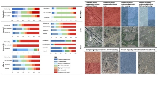
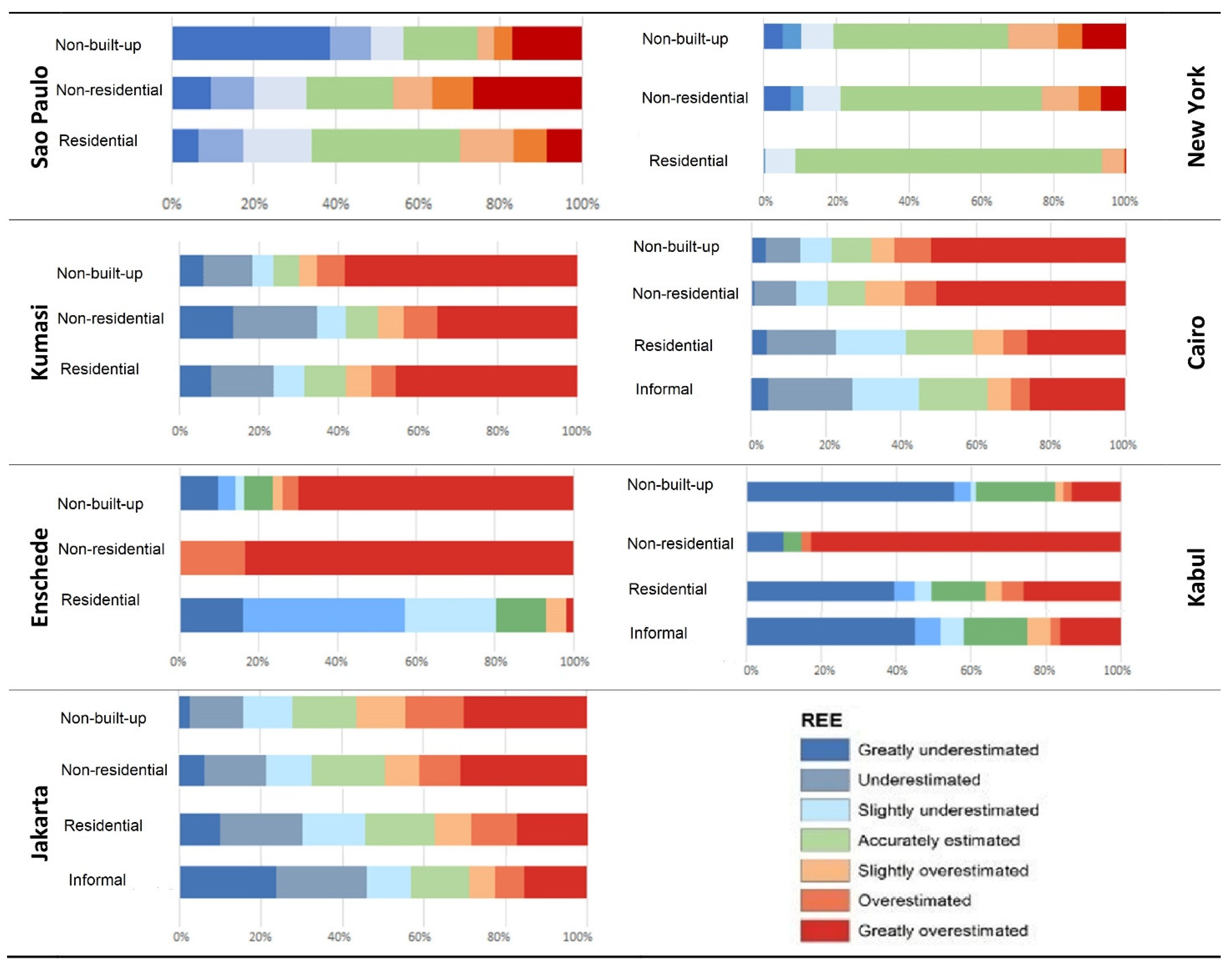
• What is the relationship between the spatial pattern of over-and underestimated areas and the types of land use?
• What are the implications for the use of presently available population data in urban growth models?

2. Gridded Population Models—Their Strengths and Limitations

Traditionally, population data are obtained through a census—official counts of all persons in a country. Census data are collected at long intervals, commonly every ten years. However, in many Low-and-Middle-Income Countries (LMICs) censuses have been interrupted, postponed or are not scheduled [16], with common causes being conflicts and, also, recently, the COVID-19 pandemic. For instance, the Democratic Republic of Congo has not had a census for 30 years, and Brazil recently postponed its 2020 census. Additionally, the census data collection frame may have biases, such as the exclusion of marginalized groups (e.g., slums, temporary settlements) [17,18]. Additionally, administrative units change over time and large aggregation units can hide heterogeneity in the area (known as the modifiable area unit problem [19]).

Global gridded population mapping approaches started in the 1990s, when population data from irregular vector formats were converted to standardized grid cells [10,20]. Global gridded population datasets use a consistent model framework (e.g., WorldPop), providing a high-resolution population count (e.g., 100 m grid cells). Most gridded dataset sets use dasymetric models to estimate the spatial distribution of population data, using available census data in combination with other spatial data (e.g., land cover) to disaggregate population counts across grid cells. They are split into top-down and bottom-up approaches. Most global population datasets are derived from top-down gridded approaches (see Appendix A); they disaggregate population counts into small grid cells (e.g., GHS-POP). Simple top-down approaches assume a uniform distribution of population within administrative units (e.g., GPWv4 [21]), while more complex approaches incorporate ancillary data to generate weights (e.g., land cover, night-time lights) for allocating population [8]. Bottom-up gridded approaches are typically based on micro-census samples and build geo-statistical relationships between population density (micro-census) and the built environment to predict population counts across grid cells of unsampled areas (Wardrop et al., 2018) (e.g., LandScan-HD or GRID3).

Many gridded population datasets are now available, which have been emerging with the data revolution, and many are open access. However, this great diversity of models leaves users often very uncertain about the advantages and limitations of individual datasets. The input data in these models are diverse, and underlying assumptions and modelling approaches affect the outcome of the gridded population dataset. For example, the grid sizes differ, ranging from 30 m to 10 km. Large grid cells better reflect the low granularity of available census data (used as the input), but are limited in reflecting the spatial variability of populations [11]. In general, gridded datasets, except for LandScan, measure the night-time population. For large cities, there can be a difference of several million between the daytime and night-time populations, as people commute to cities for work, education, etc.

Commonly used global gridded population models are summarized in Appendix A. Most of these models use the GPW as their input, which is now in its fourth version (GPWv4). GPWv4 is based on the most detailed spatial resolution census data collected between 2005 and 2014. For example, the GHS-POP uses the Global Human Settlement Layer (GHSL) and GPWv4 [22]. WorldPOP includes several covariates (e.g., night-time lights) to model population distribution using a random forest-based machine learning approach [8]. Grid3 is an emerging dataset that presently provides population data for several African countries as a bottom-up model. The historic HYDE model, based on the United Nation’s World Population Prospects and historical estimations from the literature [23,24], provides a time series of the human population with a spatial resolution of 10 km. These population models use a variety of ancillary data (e.g., built-up masks, land cover, land use, roads, infrastructure, services, night-time lights, topography and points of interest [7,9,25]) that assist in the spatial distribution of the population [8,25,26]. In general, the resolution of ancillary data influences the predictability of the model. In most cases, high-resolution data provide more reliable estimates than coarse-resolution data. However, only a few high-resolution datasets have global coverage and layers might have gaps (e.g., in rural areas) [25,27]. Commonly used ancillary data include land-cover/land-use maps from satellite images, e.g., the Global Human Settlement Layer or the Global Urban Footprint [26]. Typically, the integration of several ancillary datasets improves the accuracy of the population model [28].

Understanding the modelling approaches is an essential step in understanding the strengths and weaknesses of each dataset. As the population distribution approach disaggregates census data into grids, the uncertainties of the input data will propagate in the model. In addition, the employed modelling methods come with caveats. For example, several population models (e.g., LandScan, GHS-POP) employ regression-based models [29]. These models assume a stable relationship between population density and covariates. However, this assumption is false, and non-linear relationships are not captured [30]. Machine learning models are increasingly used for population modelling (e.g., WorldPOP). Random Forest (RF) [31], for example, can deal with high dimensional datasets and can model complex non-linear relationships. Thus, besides the census, the different input data and modelling approaches used can also impact the accuracy of the model. We have summarized their strengths, weaknesses and dependencies based on the literature (

Table 1. Strengths and weaknesses of population models reported in the literature [8,23,33,34,36,37,38] (GPWv4 is based on 2010 round of census and includes over 12,500,000 units and GPWV3 was based on 2000 round of census and includes over 375,000 input units).

Dataset Name.	Population Data/ Dependency	Strengths	Weaknesses
GPWv4	Census between 2005 and 2014	Light modelled and not affected by covariates Suitable for independent measure of population studies	Poor coverage of the spatial variability (population is evenly distributed) Overestimates population in rural areas and underestimates in urban areas
GHS-POP	GPWv4	The method is easily reproducible Global consistency	It solely depends on the GHSL to allocate population (no land-use differentiation Errors in the GHSL will propagate into the model GHSL tends to underestimate built-up in high-density areas
GRUMP	GPWv3	First global dataset to estimate population for rural and urban areas separately	The coarse resolution of the night-time data leads to overestimations in some urban areas It underperforms in estimating the spatial dynamics of population in a complex urban setting
HYDE		Includes maps of historical population estimates	Unavailability of traditional uncertainty metrics Low spatial resolution (10 km) Mostly based on urban areas
LandScan	Subnational census and administrative data	Models the ambient population The complexity of the model allows it to better capture the spatial variability of population in urban areas	Model changed between years (inconsistencies) Complex modelling approach, which varies across countries Poor performance in some rural areas due to data
HRSL	GPWv4	It provides more detailed urban and rural population estimates than GRUMP	It does not differentiate residential from other land uses Population can be allocated in industrial and commercial areas
WPE	Processed country-official data (138 countries)	Suitable for large-scale economic and trade analysis	Methodological changes each year make comparisons across time difficult
WorldPOP	GPWv4	Uses machine learning to identify significant covariates for the model Captures detailed spatial variability of population The model does not mask non-built-up areas and therefore does not produce zero population in desert and forest areas	Excluding uninhabited land compared to other datasets due to the clustering of population
LandScan HD		Performs well in data-poor regions Includes cell-level uncertainty estimate	Only available for 23 countries

). Besides the modelling approach, the main factor that influences the accuracy of top-down approaches is the census data (e.g., its aggregation scale). The more spatially disaggregated these input data are (i.e., the higher the resolution), the more precise the allocation in the grid cells [32]. The modelling approach influences the disaggregation/allocation of the population into the grid cell; many population models (e.g., GHS-POP, GRUMP) do not differentiate residential from other land uses such as commercial and industrial and, therefore, allocating population to non-residential areas. Most datasets (e.g., WorldPOP, GHS-POP) model the night-time population (census), while LandScan provides the ambient population [33]. Generally, models show poor performance in high-density urban areas (e.g., informal areas) [34,35]. This is a consequence of most spatialization methods that distribute the census population over built-up areas, including non-residential areas [11]. To deal with these limitations, recently, bottom-up approaches are being developed that directly predict population within unsampled grid cells or integrate both modelling approaches (e.g., GRID3) [2].

Given the increasing availability of population datasets, it is important to know how accurate these datasets are. The common validation approach is to compare the model estimates with authoritative population data. However, fine-resolution census datasets are not readily available at a global scale [39], nor is there an accepted method to measure the level of errors in population estimates [4,33]. Commonly used methods include the root mean square error (RMSE), mean absolute error (MAE) and mean absolute percentage error (MAPE) [9,39].

Table 2. Common causes of errors in modelling approaches and suggested solutions from literature.

Causes of Errors	Probable Causes	Recommendations	Key References
Spatial heterogeneity affects population counts	Uniform distribution assumption	Complex spatialization models are likely to perform better in complex urban distribution settings	[9,25,34]
Quality of census data	Gaps, and low spatial and temporal granularities	Combine or replace with bottom-up models	[32,33,34,41]
Quality of ancillary data	Poor ancillary data quality (errors propagate into the model)	Inspect ancillary data before using as an input Check data redundancy and covariates contribution	[7,16]
Scale effect and temporal mismatch	Data inconsistencies at spatial and temporal scale	When available, use high-resolution RS input When not, be conscious on probable uncertainties and allocate time for data corrections	[8]
Differences in regional and local characteristics	Top-down modelling approaches are less sensitive to regional characteristics Lack of reliable ancillary data with high resolution in the global level	Experiment with different ancillary datasets regarding environmental and morphological variables to better characterize the local specificities increasing the model sensitivity	[7,32]

summarizes five common causes of errors: the spatial heterogeneity of the environment (e.g., variations in population densities) [23,40]; the quality of census data (e.g., temporal and spatial resolution) [32,41]; the quality of ancillary data [42] (e.g., reliance on coarse-resolution night-time light data); the scale effect and temporal mismatch increase uncertainty (e.g., differences in data availabilities) [8]; and differences in regional and local characteristics (e.g., differences in the urbanization rate). Most HIC countries have a relatively slow rate of population growth and a more stable settlement pattern than LMICs, impacted by uncontrolled urbanization (e.g., slums). All global gridded population datasets underestimate the slum population [34].

3. Materials and Methods

To assess model uncertainties in the population allocation of the GHS-POP layer, seven cities were selected. These cities were selected for two main reasons. First, they represent a generalized world sample under the seven World Bank regions division. Second, they were selected based on the availability of spatially fine-grained local population and land-use datasets. Figure 1 shows a general overview of the approach used to analyze the city-level dataset. First, the collected datasets were inspected, cleaned and prepared for analysis. City-level datasets required a common geo-referencing system and were masked to the area of the administrative extent (as most local population datasets are only available for this extent and not for a morphologically built-up region). Next, the local population data and GHS-POP datasets were aggregated to 1 km grid cells, this being a common resolution used for global urban growth models (e.g., [43]). For the local population data and the GHS-POP data, we also included cells with zero population values in the analysis to avoid biased results.

For the error estimation, we used different error metrics (for details, see Section 3.1) and analyzed the spatial patterns of model uncertainties. A complete evaluation of each case study was performed by relating the population estimation and acquired error metrics with land use. The available land-use data for each city were reclassified into three classes, i.e., non-residential built-up, residential built-up and non-built-up. This was necessary as the available land-use data for the different cities had various levels of detail. In general, a built-up area is defined by the presence of elevated structures and buildings, while non-built-up areas mostly lack such structures (e.g., agriculture, park and forest areas) (Pesaresi et al., 2013). Residential built-up areas are dominated by residential land uses, while non-residential built-up areas are dominated by non-residential uses (e.g., industries, large infrastructures). For cities for which we had access to data, and where it was relevant, the class ‘residential’ was further split into informal and formal residential.

3.1. Accuracy Assessment Approach

Four commonly used error metrics were used to gain insights into the absolute and the relative accuracy. The root mean square error (RMSE), the mean absolute percentage error (MAPE) and the R² where utilized to understand the overall accuracy of the GHS-POP data as compared to the local population data (Bai, Wang, Wang, Gao, & Sun, 2018; Xu, Ho, Knudby, & He, 2020; Calka & Bielecka, 2020). In addition, the relative estimation error (REE) per grid was used to assess the spatial distribution of errors using the mean population values per fishnet cell (

Table 3. Error Metrics used to assess the spatial distribution of the modelled population data.

Error Metrics	Equations	Comments
Root mean square error (RMSE)	$RMSE=\sqrt{{\displaystyle {\displaystyle \sum }_{i=1}^n}\frac{{\left(y_{pred}-y_{ref}\right)}^2}{n}}$	Where ypred is the predicted/estimated value and yref the local reference value, (ypred − yref)2 = differences, squared and n is number of observations
Mean absolute percentage error (MAPE)	$MAPE=\frac{1}{n}{\displaystyle {\displaystyle \sum }_{i=1}^n}\left|\frac{y_{ref}-y_{pred}}{y_{ref}}\right|$
Relative estimation error (REE)	$REE=\frac{AEE}{y_{ref}}\times 100$	Where AEE is the absolute estimation error (ypred − yref)
Coefficient of determination (R2)	$R^2=1-\frac{RSS}{TSS}$	Where RSS is total sum of square residuals and TSS total sum of squares

).

For a detailed comparison of the two population grids, the REE was categorized into seven error classes, as shown in

Table 4. The classification scheme for Relative Error Estimation (REE).

Value Range	Category	Abbreviation
−100 to 50	Greatly underestimated	GU
−50 to 25	Underestimated	U
−25 to 10	Slightly underestimated	SU
−10 to 10	Accurately estimated	AE
10 to 25	Slightly overestimated	SO
25 to 50	Overestimated	O
50 to 100+	Greatly overestimated	GO

. A difference of +/−10% per cell was used as a threshold to define accurate estimation. The REE was used to show the spatial patterns of errors as it allows for a comparison of the difference between the GHS-POP and local population data at the grid-cell level. At the same time, the other metrics in Table 3 provided mean statistics at the city scale.

3.2. Selection of Case Studies

To support a global assessment for each of the World Bank global regions, one example city has been used (

Table 5. Selected case cities by world region.

Region	Country	City	Year of Local Population Data	Year GHS-POP	Land Use map	Informal Layer (Y/N)
East Asia and Pacific	Indonesia	Jakarta	2019	2015	2017	Y
Europe	Netherlands	Enschede and Twente region	2015	2015	2012	N
Latin America and Caribbean	Brazil	São Paulo	2010	2015	2014/20	Y
The Middle East and North Africa	Egypt	Cairo	1996	2000	2000	Y
North America	USA	New York	2010	2015	2020	N
South Asia	Kabul	Afghanistan	2015	2015	2015	Y
Sub-Saharan Africa	Ghana	Kumasi	2010	2015	2016	Y

). The selection was driven by the availability of relatively disaggregated local population data that are close to one of the reference years of the GHS layer (i.e., 1975, 1990, 2000 and 2015). The selected cities included different types (different urban morphologies), i.e., coastal (e.g., Jakarta) and inland (e.g., Enschede) cities, megacities (e.g., Sao Paulo) and secondary cities (Kumasi), economic hubs (e.g., New York) and cities with informal developments (e.g., Kabul). In cases where the local population data did not match with the exact GHS-POP reference year, the local population data were projected to make them comparable with GHS-POP using the following equations: Equation (1)—growth rate and Equation (2)—population projection.

$$r=\frac{LN \left(\frac{P_t}{P_0}\right)}{t}$$

(1)

$$P_t=P_0\times e^{rt}$$

(2)

where P_t = value at time GHS-POP time, P₀ is the value at the start, r is the rate of growth and t is the number of years.

The local population data aggregated to the 1 km grid of the GHS-POP layer was finally compared with the modelled population using the five selected error metrics (Section 3.1).

3.3. Comparison of Case Studies: Spatial Patterns of Uncertainties

To analyze the spatial patterns of uncertainties for all cities, local land-use maps were acquired. For consistency purposes, the land-use data were reclassified into residential, non-residential built-up and non-built-up. For each of these classes, the REE was calculated. This allowed for the assessment of the relationship between land-use types and uncertainties. In four cities (Kumasi, Jakarta, Kabul and Cairo), the residential class was further split into formal and informal to further investigate the different uncertainties.

4. Results

The results are presented in a comparative way; to analyze the overall patterns of errors and the particularities of individual cities.

4.1. Overall Error Estimation per Case Study

The overall error estimation in

Table 6. Overall error estimation comparison of case studies (Colors represent: red: weak model fit, orange: moderate model fit and green: strong model fit).

	Sao Paulo	Kumasi	Enschede	Jakarta	New York	Kabul	Cairo
MAPE (%)	10.7%	98.3%	−11.3%	74.4%	6.1%	−1793.7%	298.0%
RMSE	3020.6	8059.9	568.3	9814.9	896.0	5469.8	11881.9
R2	0.86	0.33	0.74	0.26	0.98	0.60	0.71
Interpretation	Strong fit of model Low error: underestimation	Weak fit of model: High error: underestimation	Strong fit of model Low error: overestimation	Weak fit of model High error: underestimation	Strong fit of model Low error: underestimation	Moderate fit of model High error: overestimation	Strong fit of model High error: underestimation

shows two distinct patterns. First of all, cities in the HICs have a better model fit, i.e., the R² values tend to be higher as compared to cities in the Low- and Middle-Income countries (LMICs). The only exception here was Sao Paulo, with an R² value of 0.86. Brazil has a very well-developed census, which is conducted on a regular basis. For the four cities in LMICs, the model exhibited a moderate to weak fit. Second, in most cities, the modelled population (GHS-POP) underestimated the local population data. This means that the modelled population tends to be lower than the actual population. However, two cities defied this trend: in Enschede and Kabul, the modelled population tended to be mostly too high. In Enschede, this occurred mainly in the outskirts of the urban area, while in Kabul it occurred more in the central locations.

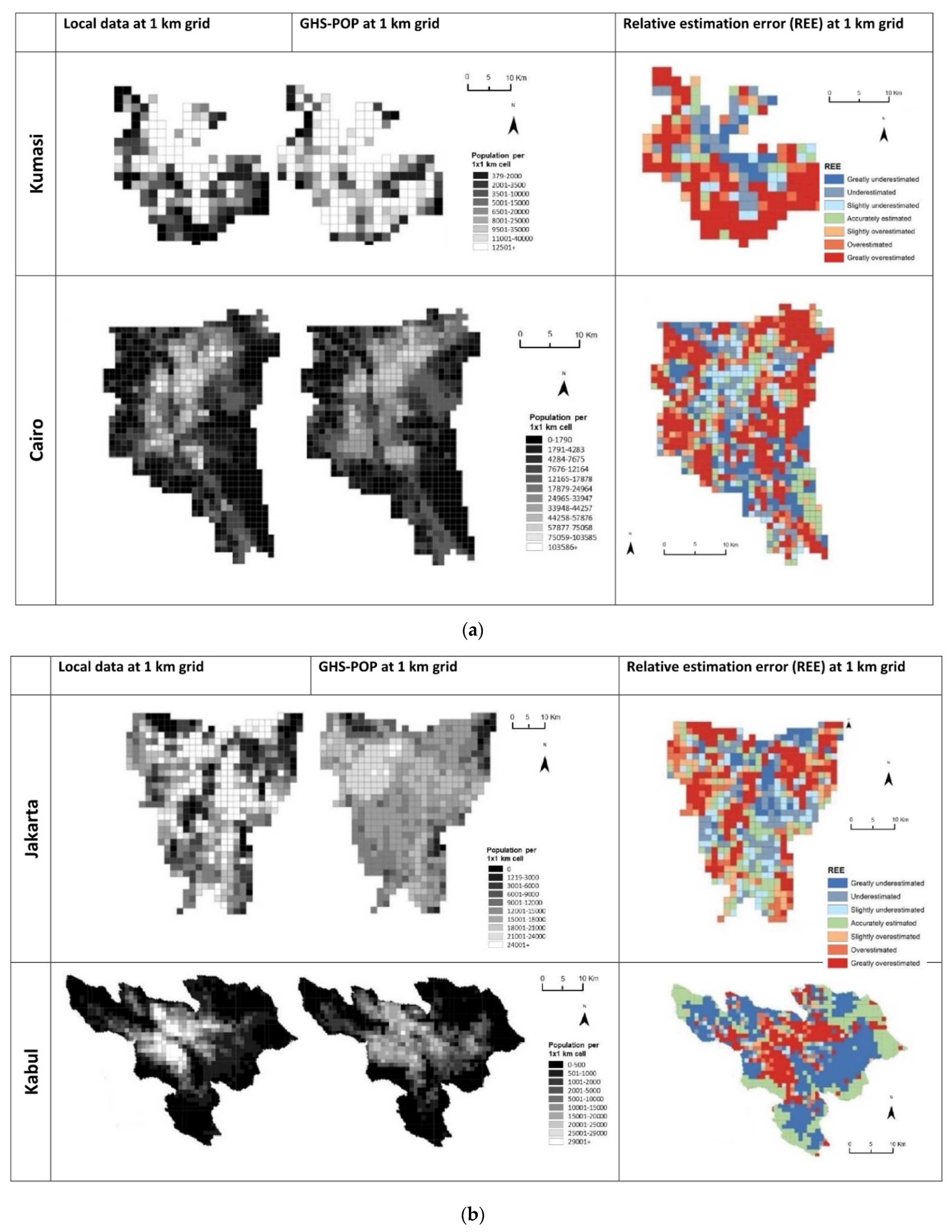
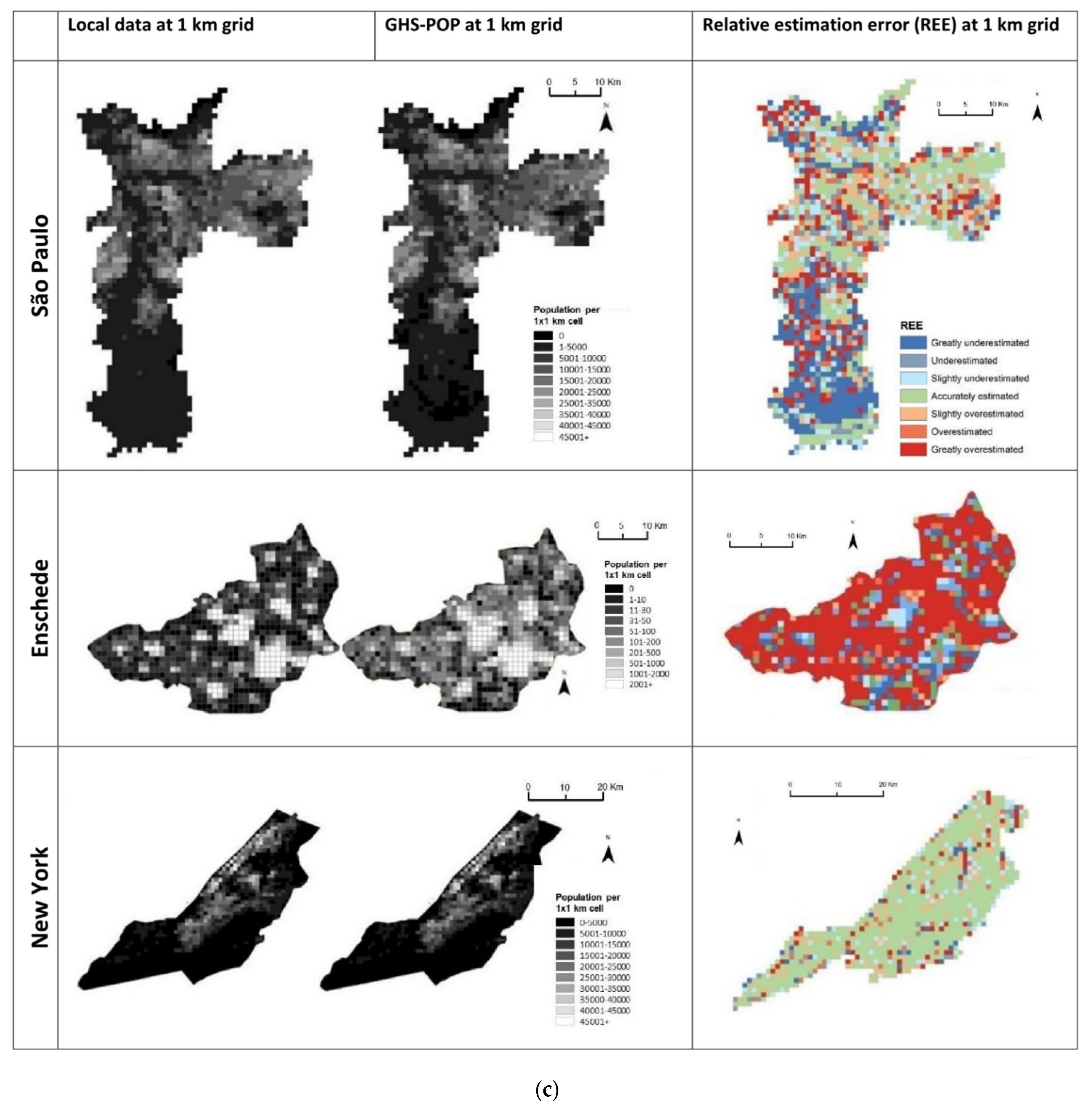
4.2. Spatial Patterns of Errors

To compare the local population data with the GHS-POP model, Figure 2a–c presents the spatial patterns of the population values (at 1 × 1 km grid cells) and the relative estimation errors (REE). It shows the population distribution at the grid level across the cities, and it reveals similar patterns between estimated and measured values. In general, the GHS-POP population distribution follows major city features. Across cities, outskirts were overestimated, while more central parts were underestimated. In several cities, the commercial and industrial areas also showed a strong overestimation, most visible in Kabul and Jakarta. For example, in Jakarta, the harbor area was highly overestimated by GHS-POP.

4.3. Land Use and Population Distribution Relationships

To further analyze the relationship between the errors and land uses, the REE was calculated for the different land-use types at the grid-cell level. The results (Figure 3) show that non-residential built-up areas tended to be overestimated. This is an obvious result of not using a land-use layer as part of the modelling approach. Generally, regions of commercial, industrial and infrastructure/transport activities (e.g., harbors) were overestimated. Non-built-up areas were also often overestimated, due to small structures being detected by the GHSL, which in many cases are not residential, or small scattered settlements with much lower population density as modelled by GHS-POP. Two cities showed different results. In Kabul and in Sao Paulo, the non-built-up areas tended to be underestimated. In both cities, scattered developments on their outskirts are not well captured by the GHSL layer. In the case of Sao Paulo, errors were caused by dense vegetation cover, and in Kabul by informal developments in step slopes (rocky terrain with little contrast between buildings and rocks). For the cities with large informal settlements (we excluded Sao Paulo as most informal areas are much smaller than 1 km²), informal areas tend to be underestimated, even at this coarse scale of analysis. Overall, we see that, due to the overestimation of the population in non-residential areas, residential and in particular high-density residential areas (such as informal areas) were underestimated.

5. Discussion

5.1. What Are the Common Issues across All Case Studies?

For the general error patterns (

Table 7. City comparison between GHS-POP and local population data.

City	Overall Conclusion	Reasons for Errors	Overall Recommendations	Correct Estimation for Residential Areas
São Paulo	GHS-POP shows an overall good prediction	overestimation of high-density areas in the city core (3D) noisy estimation for sparsely built-up areas overestimation of non-residential areas	Use of a land-use layer that allows for improved estimation of non-residential built-up areas and high-density areas (including build heights)	Correct area: 26.73%
Kumasi	GHS-POP shows an overall poor fit with the local population data	underestimation of high-density built-up areas (inner city and slums) overestimation in transition zones (mixture of non-built-up, undeveloped lands, uncompleted buildings and non-residential land use	Use of a land-use layer that allows for improved estimation of non-residential built-up areas and data on built-up densities and slum layer	Correct area: 8.9%
Enschede	Overall the GHS-POP data capture the population distribution well	overestimated areas relate to large infrastructure (harbour, airport) or industrial areas underestimation is a consequence of the overestimation (wrongly allocated population), impacting high-density areas	The inclusion of basic land use/cover (e.g., provided by the Urban Atlas) could mitigate the wrong allocation of population For multi-storey housing areas, building height information would be beneficial	Correct area: 12.0%
Jarkarta	GHS-POP has serious allocation errors and fails to accurately characterize the spatial patterns of population distribution	overestimation occurs in non-residential and non-built-up (e.g., industries, warehouses, stadiums and parks) underestimation occurs in informal areas, high densities are not well captured	The poor performance of GHS-POP can be attributed to the coarse resolution of the input population data used for Jakarta Built-up densities vary starkly in Jakarta between different land-use types, meaning the inclusion of land-use data that also differentiate between formal and informal would be beneficial	Correct area: 16.2%
New York	The GHS-POP layer provides a good depiction of the population distribution	overestimations are caused by non-residential land uses in coastal zones and harbour areas underestimation is found in high-density areas (building height)	The inclusion of basic land use/cover could mitigate the incorrect allocation of population For multi-storey housing areas, building height information would be beneficial	Correct area: 68.2%
Cairo	GHS-POP failed to accurately characterize the spatial patterns of population distribution	underestimation occurs in residential areas overestimation occurs in non-residential and non-built-up areas (e.g., agricultural areas)	The GHS-POP performs relatively well in desert areas Information on high-density and informal areas would be important to improve the GHS-POP layer	Correct area: 13.4%
Kabul	GHS-POP failed to accurately characterize the spatial patterns of population distribution	underestimation of areas in the outskirts of Kabul (e.g., agriculture areas, hillside slums) overestimation of non-residential and formal areas	The GHSL layer would require improvements to better account for built-up and non-built-up areas Use of a land-use layer could improve the estimation of non-residential built-up areas and high-density informal areas	Correct area: 27.8%

), we observed that cities in Upper-Middle-Income Countries (UMICs) and LMICs with frequent, open and well-established census data collection systems were better modelled by the GHS-POP data compared to cities with low census frequencies. Complex cities in LMICs that are dominated by large-scale informal (slum) developments had large estimation errors. The common issues observed in all case studies relate to estimation errors due to large non-residential built-up areas that were incorrectly assigned population estimates by the GHS-POP layer. Furthermore, high-density areas (e.g., informal settlements) were often underestimated. The absence of a basic land-use map in the modelling approach of the GHS-POP causes a major problem, i.e., much of the population is allocated to non-residential built-up areas while the population of high-density residential areas is underestimated. On a global average, around 25% of urban grid cells had a correctly estimated population (with +/−10%), while 75% of all urban grid cells were wrongly estimated. These numbers indicate profound uncertainties when it comes to using such data as an input for urban models, as 75% of urban areas were not well modelled in this study.

In general, scattered development on the outskirts of cities shows overestimation and underestimation (Figure 4). The sparse low-density areas are encompassed within large census units, assuming homogenous densities and not considering the settlement locations (in the census data), while the GHS-POP can better capture these density variations. However, the resolution of the GHSL layer is still too coarse to capture small-scale development and tends to over-predict built-up areas [44].

Another major problem observed with the GHS-POP data (Figure 5) relates to an overestimation of non-residential areas (e.g., large transport infrastructure, industrial areas); this overestimation contributes to an underestimation of the moderate- to high-density residential areas. Many moderate- to high-density residential areas have high-rise structures, which are not captured by the GHS-POP model.

5.2. What Are the Recommendations for Built-Up Modellers When Using the Data?

Global urban growth and built-up models require population data as an input. However, we have shown that the errors within such data have a geographic dimension. In general, based on these case studies, we observed that HIC cities and cities with good census data have, in general, much fewer model errors as compared to LMIC cities. However, for LMIC cities in particular, built-up models are very relevant for understanding the often-unplanned urban developments and for predicting future developments (Figure 6). Due to the nature of the simple binary dasymetric model for GHS-POP, these data come with caveats for built-up models. GHS-POP tends to underestimate high-density areas and overestimate sparsely populated areas [34]. A similar result has been observed for GHS-POP data in Poland and Portugal [39]. Thus, the urban population density surface has a bias. A built-up model might wrongly predict densification of central areas, where the actual density is already very saturated, while assuming population in the outskirts, where actually no or very few scattered rural developments are found. It might also predict new development in surrounding areas where actually nobody is presently living.

5.3. What Are the Recommendations for Population Modellers to Improve Their Models?

Optimally, the inclusion of land-use data would be of great benefit in solving many of the observed problems in the GHS-POP data. This would allow for a reduction in errors in built-up non-residential areas. However, land-use datasets are not (yet) readily available for many parts of the world, and, if available (e.g., https://wri-datalab.earthengine.app/view/urbanlanduse (accessed on 15 June 2022), they might not be easily comparable, may lack validation and might exclude or insufficiently capture informal developments. In principle, global land-use data are under development that allow for the masking of non-residential built-up areas (e.g., industrial areas) as well as new layers that provide an estimation of building heights (e.g., [45,46]).

To deal with the global variation in data availability, a combination of top-down and bottom-up approaches will be essential. However, despite the continuous increase in population modelling, most models are top-down. In particular, the lightly modelled top-down models (e.g., GWP, GHS-POP and GRUMP) are assumed to be more suitable at the global scale because they rely less on ancillary data and, therefore, do not have a strong dependency on input data quality (as compared to heavily modelled approaches, e.g., WorldPop). However, we have shown that even for lightly modelled population data (i.e., GSH-POP), variations in input data led to large error variations.

Bottom-up models are seen as a solution for areas with an absent or infrequent census, as such models can be built using increasingly available global spatial covariates (e.g., based on open Geospatial and Earth Observation data). However, any model assumptions should be made with care. For example, the inclusion of increasingly available building footprints (e.g., the Google Open Buildings) is promising, but large-scale omissions are observed in these datasets, particularly for high-density informal areas. Furthermore, the assumption that night-time lights show the presence of human settlement can also be misleading in areas that are not connected to the formal electricity grid. Thus, the quality of covariates varies across the globe and will determine the generalizability of any population modelling effort. Presently, the data availability and consistency of covariates are improving. These provide new opportunities for population modelling. However, there is often higher quality data available in the HICs than in LMICs, where data is often unavailable. Further studies could assess the overall model uncertainty in a way that is not constrained by census data (e.g., using micro-censuses). Efforts are needed to understand how errors inherent in different ancillary data influence the modelling process. Furthermore, newly available population data (e.g., GHS-POP July 2022 release [47]) should be compared with other even more fine-grained population data (e.g., the HRS).

6. Conclusions

Our analysis of the GHS-POP data for several cities representing the major global World Regions shows considerable differences in model fit and estimation errors. In general, the population in HIC and UMIC cities was better estimated (around 35% of the urban grid cells at 1 km were correctly estimated) with a better model fit (R² above 0.7) as compared to LMIC cities (around 15% of the urban grid cells at 1 km were correctly estimated). In most LMIC cities, the population in high-density (often informal areas) was not well captured. In addition, across all cities, the model exhibited a tendency to incorrectly allocate population to non-residential built-up areas. Furthermore, for all cities, the population in high-rise built-up areas was not well captured, as no building height information (building volumes) is used in the model. Furthermore, the population estimation of the GHS-POP was limited by the built-up mapping accuracy of the GHSL layer (e.g., large problems were observed in the case of Kabul). Thus, to improve the GHS-POP layer, it would be important to use a basic layer that restricts the allocation to residential areas. Furthermore, to improve the allocation for high-density built-up areas, a layer that provides information on slums/informal areas and basic information on building heights would be of great advantage (several such products have recently been developed).

References

1. United Nations. Demographic and Social Statistics. Available online: https://unstats.un.org/unsd/demographic-social/census/document-resources/ (accessed on 14 December 2020).
2. Boo, G.; Darin, E.; Leasure, D.R.; Dooley, C.A.; Chamberlain, H.R.; Lázár, A.N.; Tschirhart, K.; Sinai, C.; Hoff, N.A.; Fuller, T.; et al. High-resolution population estimation using household survey data and building footprints. Nat. Commun. 2022, 13, 1330. [Google Scholar] [CrossRef] [PubMed]
3. Weber, E.M.; Seaman, V.Y.; Stewart, R.N.; Bird, T.J.; Tatem, A.J.; McKee, J.J.; Bhaduri, B.L.; Moehl, J.J.; Reith, A.E. Census-independent population mapping in northern Nigeria. Remote Sens. Environ. 2018, 204, 786–798. [Google Scholar] [CrossRef] [PubMed]
4. Leyk, S.; Uhl, J.H.; Balk, D.; Jones, B. Assessing the accuracy of multi-temporal built-up land layers across rural-urban trajectories in the United States. Remote Sens. Environ. 2018, 204, 898–917. [Google Scholar] [CrossRef] [PubMed]
5. Kavvada, A.; Metternicht, G.; Kerblat, F.; Mudau, N.; Haldorson, M.; Laldaparsad, S.; Friedl, L.; Held, A.; Chuvieco, E. Towards delivering on the sustainable development goals using earth observations. Remote Sens. Environ. 2020, 247, 111930. [Google Scholar] [CrossRef]
6. United Nations Statistics Division. The Sustainable Development Goals Report. 2018. Available online: https://unstats.un.org/sdgs/report/2018/overview/ (accessed on 9 December 2019).
7. Engstrom, R.; Newhouse, D.; Soundararajan, V. Estimating Small Area Population Density Using Survey Data and Satellite Imagery: An Application to Sri Lanka; World Bank: Washington, DC, USA, 2019. [Google Scholar]
8. Lloyd, C.T.; Chamberlain, H.; Kerr, D.; Yetman, G.; Pistolesi, L.; Stevens, F.R.; Gaughan, A.E.; Nieves, J.J.; Hornby, G.; MacManus, K.; et al. Global spatio-temporally harmonised datasets for producing high-resolution gridded population distribution datasets. Big Earth Data 2019, 3, 108–139. [Google Scholar] [CrossRef] [Green Version]
9. Qiu, G.; Bao, Y.; Yang, X.; Wang, C.; Ye, T.; Stein, A.; Jia, P. Local Population Mapping Using a Random Forest Model Based on Remote and Social Sensing Data: A Case Study in Zhengzhou, China. Remote Sens. 2020, 12, 1618. [Google Scholar] [CrossRef]
10. Thomson, D.R.; Stevens, F.R.; Ruktanonchai, N.W.; Tatem, A.J.; Castro, M.C. GridSample: An R package to generate household survey primary sampling units (PSUs) from gridded population data. Int. J. Health Geogr. 2017, 16, 25. [Google Scholar] [CrossRef] [Green Version]
11. Thomson, D.R.; Rhoda, D.A.; Tatem, A.J.; Castro, M.C. Gridded population survey sampling: A systematic scoping review of the field and strategic research agenda. Int. J. Health Geogr. 2020, 19, 34. [Google Scholar] [CrossRef]
12. Schiavina, M.; Freire, S.; MacManus, K. GHS Population Grid Multitemporal (1975, 1990, 2000, 2015) R2019A; European Commission, Joint Research Centre (JRC), Eds.; European Commission: Brussels, Belgium, 2019. [Google Scholar]
13. Badmos, O.S.; Rienow, A.; Callo-Concha, D.; Greve, K.; Jürgens, C. Simulating slum growth in Lagos: An integration of rule based and empirical based model. Comput. Environ. Urban Syst. 2019, 77, 101369. [Google Scholar] [CrossRef]
14. Pérez-Molina, E.; Sliuzas, R.; Flacke, J.; Jetten, V. Developing a cellular automata model of urban growth to inform spatial policy for flood mitigation: A case study in Kampala, Uganda. Comput. Environ. Urban Syst. 2017, 65, 53–65. [Google Scholar] [CrossRef]
15. Nduwayezu, G.; Sliuzas, R.; Kuffer, M. Modeling urban growth in Kigali city Rwanda. Rwanda J. 2016, 1, 82–87. [Google Scholar] [CrossRef] [Green Version]
16. Wardrop, N.A.; Jochem, W.C.; Bird, T.J.; Chamberlain, H.R.; Clarke, D.; Kerr, D.; Bengtsson, L.; Juran, S.; Seaman, V.; Tatem, A.J. Spatially disaggregated population estimates in the absence of national population and housing census data. Proc. Natl. Acad. Sci. USA 2018, 115, 3529. [Google Scholar] [CrossRef] [PubMed] [Green Version]
17. Carr-Hill, R. Missing millions and measuring development progress. World Dev. 2013, 46, 30–44. [Google Scholar] [CrossRef]
18. Roy, D.; Lees, M.H.; Pfeffer, K.; Sloot, P. Modelling the impact of household life cycle on slums in Bangalore. Comput. Environ. Urban Syst. 2017, 64, 275–287. [Google Scholar] [CrossRef]
19. Openshaw, S. The Modifiable Areal Unit Problem; Geobooks: Norwich, UK, 1984. [Google Scholar]
20. Balk, D.L.; Deichmann, U.; Yetman, G.; Pozzi, F.; Hay, S.I.; Nelson, A. Determining Global Population Distribution: Methods, Applications and Data. In Advances in Parasitology; Hay, S.I., Graham, A., Rogers, D.J., Eds.; Academic Press: Cambridge, MA, USA, 2006; Volume 62, pp. 119–156. [Google Scholar]
21. Doxsey-Whitfield, E.; MacManus, K.; Adamo, S.B.; Pistolesi, L.; Squires, J.; Borkovska, O.; Baptista, S.R. Taking Advantage of the Improved Availability of Census Data: A First Look at the Gridded Population of the World, Version 4. Pap. Appl. Geogr. 2015, 1, 226–234. [Google Scholar] [CrossRef]
22. Freire, S.; Macmanus, K.; Pesaresi, M.; Doxsey-Whitfield, E.; Mills, J. Development of New Open and Free Multi-Temporal Global Population Grids at 250 m Resolution; Geospatial Data in a Changing World; Association of Geographic Information Laboratories in Europe (AGILE) (Organiser); AGILE: Helsinki, Finland, 2016. [Google Scholar]
23. Chen, R.; Yan, H.; Liu, F.; Du, W.; Yang, Y. Multiple Global Population Datasets: Differences and Spatial Distribution Characteristics. ISPRS Int. J. Geo-Inf. 2020, 9, 637. [Google Scholar] [CrossRef]
24. McEvedy, C.; Jones, R. Atlas of World Population History; Pengium Books Ltd.: New York, NY, USA; Allen Lane: New York, NY, USA, 1979. [Google Scholar]
25. Ye, T.; Zhao, N.; Yang, X.; Ouyang, Z.; Liu, X.; Chen, Q.; Hu, K.; Yue, W.; Qi, J.; Li, Z.; et al. Improved population mapping for China using remotely sensed and points-of-interest data within a random forests model. Sci. Total Environ. 2019, 658, 936–946. [Google Scholar] [CrossRef]
26. Stevens, F.R.; Gaughan, A.E.; Nieves, J.J.; King, A.; Sorichetta, A.; Linard, C.; Tatem, A.J. Comparisons of two global built area land cover datasets in methods to disaggregate human population in eleven countries from the global South. Int. J. Digit. Earth 2020, 13, 78–100. [Google Scholar] [CrossRef]
27. Kit, O.; Lüdeke, M.; Reckien, D. Defining the bull’s eye: Satellite imagery-assisted slum population assessment in Hyderabad, India. Urban Geogr. 2013, 34, 413–424. [Google Scholar] [CrossRef]
28. Schwarz, N.; Flacke, J.; Sliuzas, R.V. Modelling the impacts of urban upgrading on population dynamics. Environ. Model. Softw. 2016, 78, 150–162. [Google Scholar] [CrossRef]
29. Wu, C.; Murray, A.T. Population Estimation Using Landsat Enhanced Thematic Mapper Imagery. Geogr. Anal. 2007, 39, 26–43. [Google Scholar] [CrossRef]
30. Roni, R.; Jia, P. An Optimal Population Modeling Approach Using Geographically Weighted Regression Based on High-Resolution Remote Sensing Data: A Case Study in Dhaka City, Bangladesh. Remote Sens. 2020, 12, 1184. [Google Scholar] [CrossRef] [Green Version]
31. Breiman, L. Random Forests. Mach. Learn. 2001, 45, 5–32. [Google Scholar] [CrossRef] [Green Version]
32. Gaughan, A.E.; Stevens, F.R.; Huang, Z.; Nieves, J.J.; Sorichetta, A.; Lai, S.; Ye, X.; Linard, C.; Hornby, G.M.; Hay, S.I.; et al. Spatiotemporal patterns of population in mainland China, 1990 to 2010. Sci. Data 2016, 3, 160005. [Google Scholar] [CrossRef] [PubMed]
33. Leyk, S.; Gaughan, A.E.; Adamo, S.B.; de Sherbinin, A.; Balk, D.; Freire, S.; Rose, A.; Stevens, F.R.; Blankespoor, B.; Frye, C.; et al. The spatial allocation of population: A review of large-scale gridded population data products and their fitness for use. Earth Syst. Sci. Data 2019, 11, 1385–1409. [Google Scholar] [CrossRef] [Green Version]
34. Thomson, D.R.; Gaughan, A.E.; Stevens, F.R.; Yetman, G.; Elias, P.; Chen, R. Evaluating the Accuracy of Gridded Population Estimates in Slums: A Case Study in Nigeria and Kenya. Urban Sci. 2021, 5, 48. [Google Scholar] [CrossRef]
35. Kuffer, M.; Persello, C.; Pfeffer, K.; Sliuzas, R.; Rao, V. Do we underestimate the global slum population? In Proceedings of the 2019 Joint Urban Remote Sensing Event (JURSE), Vannes, France, 22–24 May 2019; pp. 1–4. [Google Scholar]
36. Sliuzas, R.; Kuffer, M.; Kemper, T. Assessing the quality of Global Human Settlement Layer products for Kampala, Uganda. In Proceedings of the 2017 Joint Urban Remote Sensing Event (JURSE), Dubai, United Arab Emirates, 6–8 March 2017; pp. 1–4. [Google Scholar]
37. Aubrecht, C.; Gunasekera, R.; Ungar, J.; Ishizawa, O. Consistent yet adaptive global geospatial identification of urban–rural patterns: The iURBAN model. Remote Sens. Environ. 2016, 187, 230–240. [Google Scholar] [CrossRef] [Green Version]
38. Gunasekera, R.; Ishizawa, O.; Aubrecht, C.; Blankespoor, B.; Murray, S.; Pomonis, A.; Daniell, J. Developing an adaptive global exposure model to support the generation of country disaster risk profiles. Earth-Sci. Rev. 2015, 150, 594–608. [Google Scholar] [CrossRef] [Green Version]
39. Calka, B.; Bielecka, E. GHS-POP Accuracy Assessment: Poland and Portugal Case Study. Remote Sens. 2020, 12, 1105. [Google Scholar] [CrossRef] [Green Version]
40. Azar, D.; Engstrom, R.; Graesser, J.; Comenetz, J. Generation of fine-scale population layers using multi-resolution satellite imagery and geospatial data. Remote Sens. Environ. 2013, 130, 219–232. [Google Scholar] [CrossRef]
41. Freire, S.; Schiavina, M.; Florczyk, A.J.; MacManus, K.; Pesaresi, M.; Corbane, C.; Borkovska, O.; Mills, J.; Pistolesi, L.; Squires, J.; et al. Enhanced data and methods for improving open and free global population grids: Putting ‘leaving no one behind’ into practice. Int. J. Digit. Earth 2020, 13, 61–77. [Google Scholar] [CrossRef] [Green Version]
42. Uhl, J.H.; Zoraghein, H.; Leyk, S.; Balk, D.; Corbane, C.; Syrris, V.; Florczyk, A.J. Exposing the urban continuum: Implications and cross-comparison from an interdisciplinary perspective. Int. J. Digit. Earth 2020, 13, 22–44. [Google Scholar] [CrossRef] [PubMed]
43. Van Huijstee, J.; Van Bemmel, B.; Bouwman, A.; Van Rijn, F. Towards an Urban Preview: Modelling Future Urban Growth with 2UP; PBL Netherlands Environmental Assessment Agency: The Hague, The Netherlands, 2018. [Google Scholar]
44. Aguilar, R.; Kuffer, M. Cloud Computation Using High-Resolution Images for Improving the SDG Indicator on Open Spaces. Remote Sens. 2020, 12, 1144. [Google Scholar] [CrossRef] [Green Version]
45. Pesaresi, M.; Corbane, C.; Ren, C.; Edward, N. Generalized Vertical Components of built-up areas from global Digital Elevation Models by multi-scale linear regression modelling. PLoS ONE 2021, 16, e0244478. [Google Scholar] [CrossRef]
46. Li, M.; Koks, E.; Taubenböck, H.; van Vliet, J. Continental-scale mapping and analysis of 3D building structure. Remote Sens. Environ. 2020, 245, 111859. [Google Scholar] [CrossRef]
47. Schiavina, M.; Freire, S.; MacManus, K. GHS-POP R2022A-GHS Population Grid Multitemporal (1975–2030); European Commission, Joint Research Centre (JRC), Eds.; European Commission: Brussels, Belgium, 2022. [Google Scholar]
Figure 1. Methodology flowchart.
Ijgi 11 00403 g001
Figure 2. Average population count in a 1 × 1 km grid distribution for local and GHS-POP data and spatial distribution of relative estimation error (REE): (a) African cities, (b) Asian cities, (c) American and European cities.
Ijgi 11 00403 g002aIjgi 11 00403 g002b
Figure 3. Land-use maps and percentages of each REE range per land-use category.
Ijgi 11 00403 g003
Figure 4. Sao Paulo, example of overestimation in a low-density area by the GHS-POP.
Ijgi 11 00403 g004
Figure 5. Examples of very greatly over- and underestimated areas in Enschede.
Ijgi 11 00403 g005
Figure 6. Examples of very greatly over- and underestimated areas in Kabul.
Ijgi 11 00403 g006