Abstract
High-precision dynamic traffic noise maps can describe the spatial and temporal distributions of noise and are necessary for actual noise prevention. Existing monitoring point-based methods suffer from limited spatial adaptability, and prediction model-based methods are limited by the requirements for traffic and environmental parameter specifications. Road surveillance video data are effective for computing and analyzing dynamic traffic-related factors, such as traffic flow, vehicle speed and vehicle type, and environmental factors, such as road material, weather and vegetation. Here, we propose a road surveillance video-based method for high-precision dynamic traffic noise mapping. First, it identifies dynamic traffic elements and environmental elements from videos. Then, elements are converted from image coordinates to geographic coordinates by video calibration. Finally, we formalize a dynamic noise mapping model at the lane level. In an actual case analysis, the average error is 1.53 dBA. As surveillance video already has a high coverage rate in most cities, this method can be deployed to entire cities if needed.
1. Introduction
With rapid urbanization and the development of transportation, traffic noise has become a critical environmental issue worldwide. It has been reported that more than 125 million people are exposed to excessive road traffic noise in Europe alone [1]. Traffic noise has both psychosocial and physiological effects on exposed people [2,3,4], and the WHO has listed it as the second largest environmental threat to health [5]. Most countries and regions, including the United States [6], the European Union countries [7], and China [8], have formulated policies and invested considerable economic resources to mitigate excessive traffic noise. There is an urgent need to control urban traffic noise.
Noise maps can reflect the spatial distribution of noise and be used to prevent excessive noise exposure [9]. Considerable efforts have been made to map traffic noise from a spatial perspective through noise estimation of single vehicles [10], 3D noise models [11] and urban scale noise mapping [12]; from a temporal perspective through dynamic noise mapping [13,14] and acceleration noise computing [15]; and from a tool perspective through an open-source noise mapping tool [16]. Because traffic parameters (such as traffic flow volume and speed) and noise propagation parameters (e.g., weather parameters) are dynamic, noise tends to fluctuate greatly over time. Dynamic noise maps can describe the changes in noise over time and space. In actual environmental noise monitoring, such as in schools and residential areas, dynamic noise mapping is necessary for noise control. Several monitoring point-based and noise prediction model-based dynamic noise mapping projects have been implemented. Regarding the monitoring point-based method, CENSE (characterization of urban sound environments) [17] in France and DYNAMAP (dynamic acoustic mapping) [14] of the European Commission are recent examples. These projects have attempted to use low-cost sensors to generate dynamic noise maps. However, because the abundance and spatial distribution of noise monitoring equipment are limited, high precision and large coverage are difficult to achieve simultaneously. Thus, mapping large areas of noise with monitoring equipment is time consuming and expensive.
Regarding noise prediction model-based methods, dynamic traffic and environmental parameters are required as inputs. The existing methods of establishing parameters can be divided into three types: practical surveys, model simulations and statistical analyses of floating vehicle data. However, practical surveys are expensive and time-consuming in large areas, and model simulation and floating vehicle data are limited in temporal resolution and accuracy and cannot directly output environmental parameters. Therefore, dynamic traffic noise mapping remains challenging.
Road surveillance video data have been used to efficiently analyze dynamic traffic information in dynamic vehicle detection, vehicle tracking, vehicle behavior analysis and vehicle interaction assessment [18]. In addition, similar to street-view images, road videos record a variety of types of environmental information in the road environment that can be used to model the noise propagation process. Considerable efforts have been made to extract environmental information, such as the road material [19], local vegetation types [20] and weather conditions [21,22], from road images. Several recent studies have explored video data as inputs to noise prediction models. In [23], road video was used to extract the required traffic parameters, including vehicle number, type and speed, for a noise prediction model. However, it could not extract environmental factors from the video, and dynamic noise maps were not constructed.
In this study, we propose a road surveillance video-based method for dynamic traffic mapping. In the method, we formulate a dynamic traffic noise model at the lane scale considering the effect of noise propagation. Both dynamic traffic parameters (such as the traffic flow volume, vehicle speed and vehicle type) and noise propagation parameters (such as the road material, weather conditions, vegetation type and sound barriers) are specified directly from road video. From a temporal perspective, dynamic traffic parameters and noise propagation parameters can be directly specified from road video. Thus, dynamic noise maps are available. From a spatial perspective, video can be used to specify traffic parameters at the lane scale. Based on high temporal and spatial resolution traffic and noise propagation parameters, high-precision traffic noise maps can be obtained. Considering that road surveillance video already has high coverage in most cities, it can cover the entire urban scale if needed. Thus, this method can efficiently adapt to dynamic traffic mapping at large urban scales. In the next section, we summarize the related works regarding the measurement and prediction of traffic noise. We then introduce the proposed dynamic noise mapping method and present the details of mathematically formulizing and algorithmically specifying dynamic traffic parameters and environmental parameters from road video data in Section 3. In the fourth section, we evaluate our method based on an actual road in Nanjing, China, and compare the model results with the survey results obtained with professional sound measurement equipment. We discuss the advantages and limitations of the method in the fifth section. Finally, we conclude the paper with a summary of the key contributions and outline future activities in Section 6.
2. Related Work
Traffic noise can be divided according to the mode of transport into road noise, railway noise, water noise and aircraft noise [24]. Road traffic noise refers to the noise generated by vehicles driving on roads; it is the most dominant source of environmental noise. The available methods for road traffic noise mapping can be generally divided into two categories: monitoring point-based methods and prediction model-based methods [25].
2.1. Monitoring Point-Based Methods
To monitor noise near particular buildings and facilities, such as construction sites and parks, noise monitoring equipment can be installed. Such equipment can monitor noise levels with high precision and in real time. With GIS and spatial interpolation methods, noise maps can be obtained within a certain range. For example, [26] used kriging interpolation to map the temporal and spatial distributions of traffic noise pollution. The authors of [27] analyzed the correlation between noise level and road network density and implemented inverse distance weighting (IDW) interpolation to analyze the distribution of noise. The authors of [28] analyzed the limitations of common interpolation methods and proposed using mobile noise measurements for noise mapping. The authors of [29] integrated smartphone-based noise data into the strategic noise mapping process.
Some researchers performed dynamic noise mapping based on the patterns of noise variations observed at monitoring points. The authors of [13] considered the temporal and spatial patterns of noise and monitored the variations in noise sources for dynamic noise mapping. The authors of [14] synthesized the variations in average noise levels at multiple stations over time for dynamic traffic noise mapping in Milan. To reduce the dependence on the distribution of noise monitoring points in large areas, [30] combined monitored acoustic data with traffic and weather data to perform noise simulation.
The above methods produced dynamic traffic noise maps within a certain range; however, because noise monitoring equipment is too expensive to broadly deploy over large areas, the number and spatial distribution of monitoring points is generally limited; moreover, sound propagation is anisotropic. Environmental factors, such as weather, buildings, vegetation and sound barriers, can affect noise propagation [31]. Overall, it is time-consuming and expensive to perform large-scale noise mapping based on information from monitoring points.
2.2. Prediction Model-Based Methods
Many efforts have been made to develop traffic noise prediction models. The most commonly used models include the FHWA model [32], which calculates the maximum sound pressure level Leq of passing vehicles at a reference distance of 15 m and is based in the US; the CoRTN model [33], which estimates the noise level L10 at 1 h and 18 h reference times at a distance of 10 m from the nearest lane of a highway and is based in the UK; the RLS90 model [34], which calculates the noise level LeqA at a distance of 25 m from the center of a road lane and is based in Germany; and the CNOSSOS model [7], which is a harmonized methodological framework for the mapping of road traffic, railway traffic, aircraft and industrial noise and is based in the EU. The advantages of prediction-model-based methods, compared to monitoring-sensor-based methods, include ease of implementation and scaling, especially over large regions. These models generally focus on vehicle noise levels combined with various influential factors, such as traffic factors (traffic flow, vehicle speed and vehicle type) and propagation factors (road material, weather conditions, vegetation types and sound barriers) [31]. Notably, the specification of traffic parameters is crucial in noise models. The existing traffic parameter assignment methods for noise mapping can be divided into three types: practical surveys, traffic model simulations and statistical analyses of floating vehicle data. The authors of [35] used actual traffic flows determined through a survey and the vehicle types and traffic flows simulated with a traffic model to establish a noise map of a building facade area based on the FHWA model. The authors of [12] obtained vehicle types and traffic flows through traffic surveys, analyzed the average traffic flows on different types of roads, and performed traffic noise mapping based on the RLS90 model. Due to the need to specify traffic parameters, it is time-consuming and expensive to perform dynamic noise mapping based on practical surveys.
Some studies have used floating car data to directly specify traffic parameters in noise models. For example, [36] specified dynamic road traffic parameters based on GPS data and vehicle speed–density models and created daytime and nighttime traffic noise maps of Guangzhou. The authors of [25] used the average speed data collected by GPS and an electronic map to analyze the regression relationship between the noise level and vehicle speed and established an hourly dynamic noise map. However, it is almost impossible to obtain and analyze GPS data from all vehicles on the road, which is why some methods use vehicle speed–density models to estimate traffic flows [36]. The temporal resolution and accuracy of traffic model simulations are limited when specifying traffic parameters. Furthermore, GPS data can only be used to estimate traffic parameters and cannot be applied to determine the environmental factors that affect noise propagation, such as the road material, weather conditions, and local vegetation types.
From the above discussion, the monitoring point-based method provides high accuracy and is dynamic, but it is expensive and time consuming to obtain a wide range of urban noise data due to the heterogeneity of noise. The existing prediction model-based methods consider the physical propagation of noise, and noise maps can be established over a wide range. However, directly specifying dynamic traffic parameters and environmental parameters remains an issue in these methods.
3. Method
3.1. Method Overview
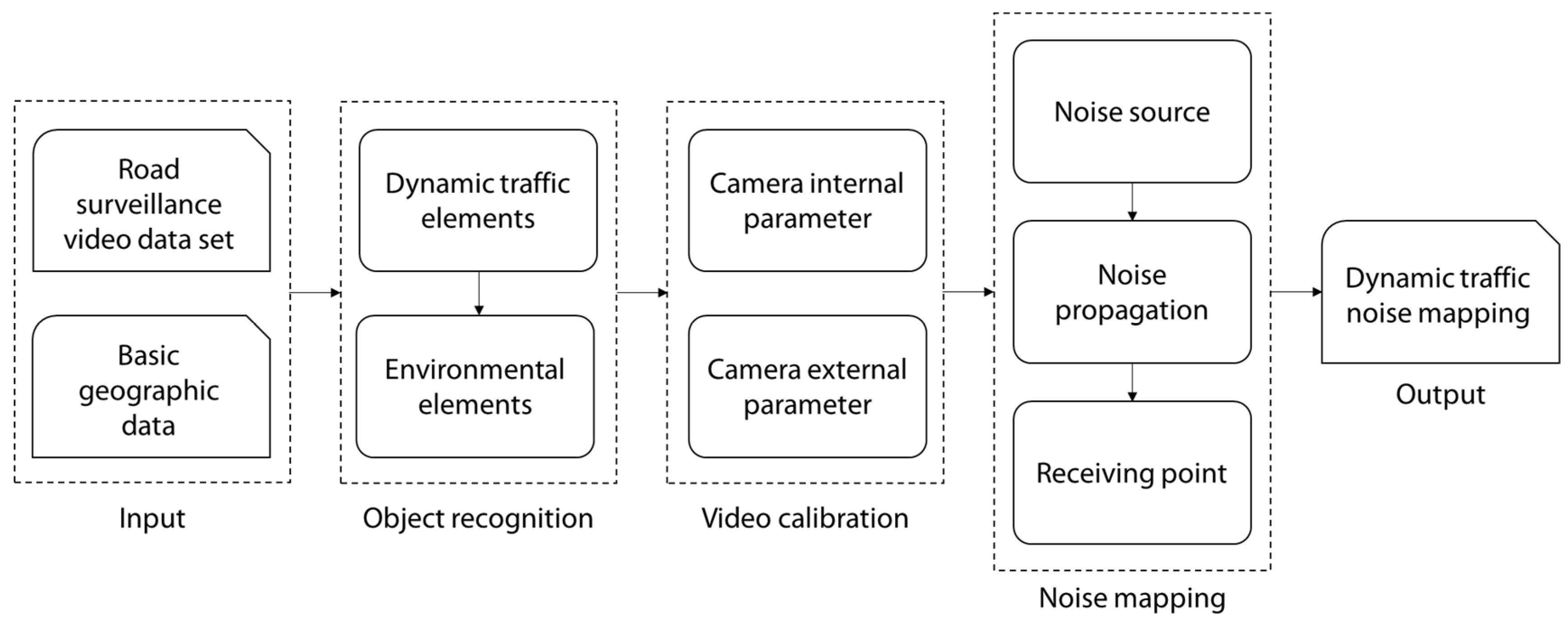
In this paper, a road surveillance video-driven method for dynamic traffic noise mapping is proposed. Figure 1 illustrates the processing of dynamic noise mapping based on road surveillance video. Our goal is not to develop a new noise prediction model but to extract the parameters required by the traffic noise model from video for dynamic noise mapping. For a certain area, road surveillance video and basic geographic data, such as road and building data, are used as inputs. First, object recognition is performed for traffic elements (vehicle trajectories) and environmental elements (road materials, weather conditions and vegetation types). Second, the elements are converted from image coordinates to geographical coordinates by video calibration. Based on the basic geographic data that are input, a vehicle trajectory is matched with the appropriate road segments to extract the traffic parameters required for noise prediction. Then, noise mapping is performed based on the sound pressure level at the source, noise propagation correction and data interpolation at receiving points. Dynamic traffic noise maps can be obtained by inputting road videos from different time periods.
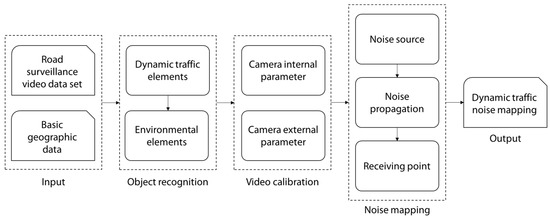
Figure 1.
Overview of the dynamic traffic noise mapping model based on road surveillance video data.
In the most common noise prediction models, such as the FHWA, CoRTN, RLS90 and CNOSSOS models, the sound pressure level at a receiving point is calculated based on the sound pressure level at the noise source and various noise propagation corrections. Considering the differences in noise sources and propagation modeling, these models are applicable to different road conditions. The Chinese criterion model of the Technical Guidelines for Noise Impact Assessment (HJ 2.4-2009) and (HJ 2.4-2021) is adapted from the FHWA model. However, the FHWA model assumes that vehicle speed is constant and is applied for straight roads such as highways. The CoRTN model is applicable to long lines of free-flowing traffic. The sound propagation aspect of the CNOSSOS model, a recent model, has yet to be thoroughly tested and validated with regard to accuracy [31]. The RLS90 model considers vehicle speed and sound barriers in detail. Existing studies have shown that the RLS90 model is suitable for complex road environments inside cities [12]. Thus, we modeled dynamic traffic noise mapping based on the RLS90 model. In Section 3.2, the conceptual framework of the RLS90 model is presented, and the required dynamic traffic and environmental parameters are analyzed. In Section 3.3, the specific process of dynamic noise mapping based on road surveillance video is described.
3.2. Noise Prediction Model
What traffic and environmental parameters are required for noise prediction models? We illustrate the conceptual framework of the RLS90 noise prediction model and analyze the required traffic parameters and environmental parameters. Similar to most noise prediction models, the RLS90 model focuses on two factors: the level of noise at the source and the attenuation of noise propagation. These factors are introduced in the following sections.
3.2.1. Level of Noise at the Source
With continuous traffic flows, roads can be regarded as linear noise sources, as shown in Figure 2. The RLS90 model involves the superposition of the near-lane noise level Ln and far-lane noise level Lf to obtain the multilane noise level Lm. For a single lane, its noise level Ls is split into a number of segmented noise sources per unit length Li, denoted as follows:
where segment noise level Li is calculated by adding the noise level at the road segment Li,E and the noise propagation correction Dp.
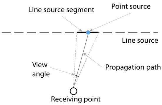
Figure 2.
Road noise source and noise segment (modified from [7]).
Specifically, the noise level of a certain road segment is mainly affected by dynamic traffic parameters associated with the road segment; these parameters include the traffic flow volume, vehicle speeds and vehicle types. In addition, road materials are considered.
3.2.2. Noise Propagation
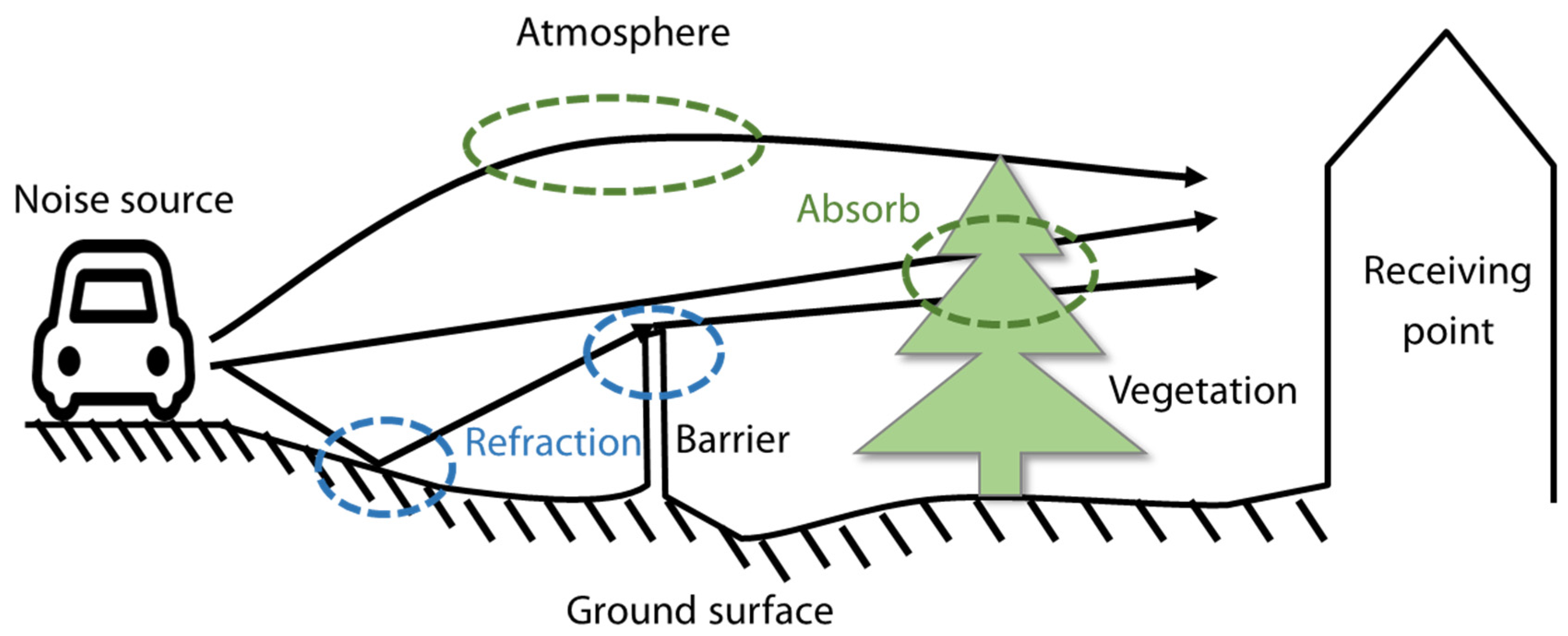
In noise propagation, the noise level can be attenuated through air absorption, ground reflection, barrier refraction and vegetation absorption [31]. Figure 3 shows an overview of the traffic noise propagation process.
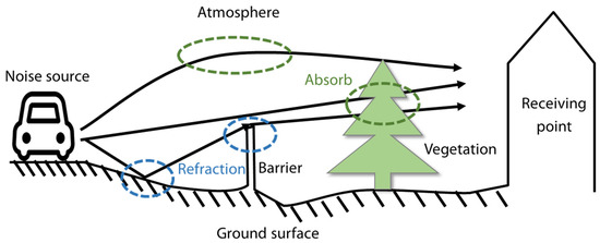
Figure 3.
Overview of the traffic noise propagation process (modified from [37]).
The RLS90 model considers correction factors for distance attenuation, ground surface absorption and sound barrier attenuation. Here, the correction factors for weather and vegetation absorption are added. Thus, sound propagation correction Dp is denoted as
where Dl is the noise source correction factor for a segment of a given length, Dd is the distance attenuation correction factor, Dg is the ground absorption correction factor, Db is the barrier correction factor, Dw is the weather correction factor, and Dveg is the vegetation correction factor.
3.3. Video-Based Traffic Noise Mapping
Based on the above conceptual noise prediction model, we propose a video-based traffic noise mapping method that includes object recognition, video calibration, and noise mapping. The detailed discussion is as follows.
3.3.1. Object Recognition
Object recognition is performed to identify dynamic traffic elements and environmental elements in road surveillance videos.
(1) Dynamic traffic elements
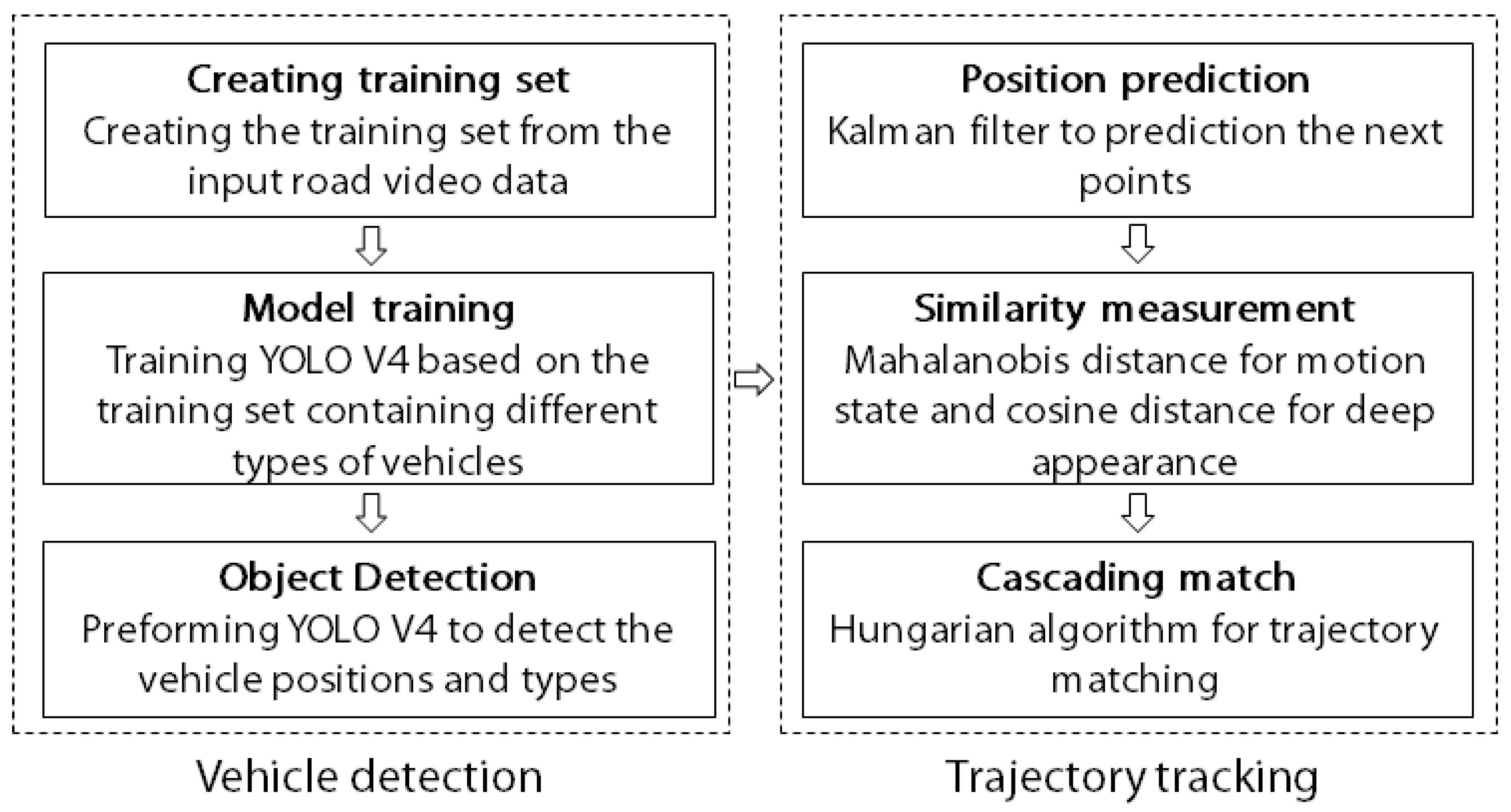
Traffic elements are the most important parameters in noise prediction models. High-precision dynamic traffic parameters are crucial for noise mapping. In the above conceptual model of noise sources, the required traffic parameters include the traffic flow volume, vehicle speeds and vehicle types. Many efforts have been made to analyze traffic information and even vehicle behavior based on video data [38,39]. Here, a two-step process is introduced to identify traffic elements in videos and perform vehicle detection and trajectory tracking, as shown in Figure 4.
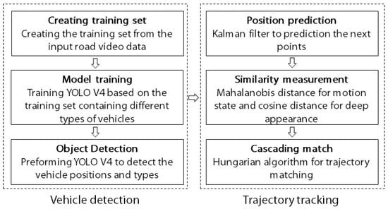
Figure 4.
Processing of extracting dynamic traffic elements based on road video data.
Vehicle detection is performed to extract the position and type of vehicle from each frame of a video. With the rapid development of image processing, many efficient multiobjective detection methods have been proposed. Here, we use the deep-learning-based object detection method YOLO (you only look once) V4 for vehicle detection from video [40]. It is reported to be approximately 10% more accurate than the previous generation general-purpose video recognition model. Benefitting from GPU-accelerated computations and learning based on a large number of samples, vehicle locations can be detected in real time, and vehicle types can be determined with high precision. The specific implementation is as follows: first, a training set is created from the input road video data. The training set contains certain numbers of cars, buses, and trucks. Then, YOLO V4 is trained with the training set containing information for different types of vehicles. Finally, YOLO V4 is used to detect the vehicle positions and types. The j-th detected vehicle in the i-th frame can be denoted
where type and confidence denote the vehicle type (e.g., car, bus or truck) and the confidence score of the detected vehicle. u and v are the vehicle positions in the image, and w and h are the width and height of the bounding box of the vehicle, respectively.
Trajectory tracking is used to identify the trajectories of objects based on their motion state in different video frames. Common trajectory tracking algorithms include object modeling-based, correlation filtering-based, and deep learning-based algorithms [41]. Here, we use a deep sorting algorithm for vehicle trajectory tracking [42]. This multiobjective tracking algorithm is based on deep object features and provides high robustness. First, a Kalman filter is used to predict the position of a detected trajectory. Then, the Mahalanobis distance of the motion state and cosine distance of the deep appearance descriptor are calculated to measure the similarity between a new object and the detected trajectory. Finally, the Hungarian algorithm is used to perform cascaded matching. After trajectory tracking, the movement trajectories of vehicles in the analyzed video can be determined.
(2) Environmental elements
The environmental elements that influence the source and propagation of traffic noise include weather conditions, road materials and vegetation types. Compared with traffic elements in a video, these elements can be regarded as static background elements in specific image frames. It is difficult to identify these parameters directly from video. Therefore, we first implement image segmentation to separate the corresponding environmental element regions from the video. Then, these elements are classified separately. Image segmentation is performed to extract interesting and easy-to-analyze regions of an image through image processing [43]. Deep learning-based image segmentation has been used in many applications, such as scene assessment, medical image analysis and video surveillance, due to its strong adaptability [44]. Here, we select PSPNet (Pyramid Scene Parsing Network) to separate the air, road and vegetation areas in videos [45]. This model can aggregate different image region-based contexts to obtain global image information and has achieved excellent performance for various datasets. Figure 5 is an example of image segmentation based on road video data. The blue area in Figure 5b is sky, the green area is vegetation, and the purple area is road. Then, we extract the environmental factors needed for the model from the image segmentation results.
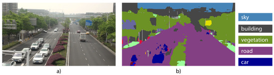
Figure 5.
Example of image segmentation based on road video data. (a) Road video example and (b) the image semantic separation result.
Weather. Many weather classification datasets and image-based weather classification methods are publicly available, such as filtering-based, machine learning-based and deep learning-based methods [46]. Notably, [21] proposed a collaborative learning framework to classify weather by analyzing multiple weather cues during learning and classification. With ten thousand weather image training data samples, the model displayed good adaptability. Here, the method of [21] is adopted to classify weather for extracted sky areas, including sunny, cloudy and rainy conditions.
Road material. Many efforts have been made to extract road material from remote sensing images [19]. Extracting road material from video data is similar to extracting information from true color remote sensing images. Here, we use Yang’s method [47] to classify road material in different road areas. Yang’s method first extracts the multidimensional features of the road, such as the HSV color, local texture and gray level cooccurrence matrix (GLCM). Then, a support vector machine (SVM) algorithm is used to classify the materials. Here, we classify road materials into four types: asphalt, cement, porous asphalt concrete and other materials.
Vegetation. Considerable efforts have been made to classify vegetation in remote sensing images. In recent research, a machine learning-based classification method was introduced and used for vegetation classification from street-view images [20]. Vegetation classification based on road videos is similar to vegetation classification from street-view images. Considering the limitation regarding the number of classification samples, we use an SVM algorithm to further classify different areas of vegetation [48]. Here, vegetation is classified into three categories: trees, shrubs and lawns.
Based on the above process, we extracted important environmental elements from road surveillance videos.
3.3.2. Video Calibration
The objects identified in road surveillance videos are associated with specific image coordinates but cannot be used to measure distance. To determine vehicle speeds and the vegetation distribution, video calibration is introduced. Video calibration converts an object from image coordinates to 3D geographic coordinates [49]. Assuming a 3D point M in geographic coordinates is (Xw, Yw, Zw), the calibration process converts M to point M’ (Xc, Yc, Zc) in camera coordinates and to m(u, v) in the image. These transformations can be formulated as follows:
where fx and fy are the focal lengths of the camera along the u and v axes, u0 and v0 are the principal point coordinates corresponding to the image coordinates, R is the camera’s rotation matrix in geographic space, and t is the camera’s translation vector in geographic space.
The focal lengths of the camera and principal point coordinates are only related to the internal structure of the camera and form the camera’s internal parameter matrix K. Correspondingly, R and t can be regarded as the camera’s external parameters. In the driving process, the vehicle height is roughly unchanged. It is assumed that the vehicle is in a plane and of height 0; that is, Zw = 0. Then, the relationship between point m in the image coordinates and point M in the geographic coordinates can be denoted as
Here, the internal parameter matrix of the camera is determined by the commonly used checkerboard method [50]. Using a special checkerboard calibration approach, corner points are automatically extracted from the calibration board. Based on a series of calibration board points and the corresponding image points, the internal parameter matrix K can be obtained.
Obtaining the external parameter matrix can be regarded as solving a perspective-n-points (PnP) problem. Here, the EPnP algorithm [51] is implemented to determine the external camera parameters. This algorithm converts all the reference points used for camera calibration into four virtual control points and then calculates the external parameters R and t of the camera based on the geographic coordinates and image coordinates of the control points. Then, the geographic coordinates of all the vehicle points and the vegetation distribution are calculated.
Next, the trajectory points are matched to road segments according to the nearest distance. Through the analysis of the trajectories of each lane, traffic parameters, including the vehicle type proportion P, traffic flow volume F and speeds of different types of vehicles vcar and vheavy, can be obtained at the lane level. In addition, environmental parameters, including the road material rm, weather type and vegetable width wveg and type αveg, can be determined.
3.3.3. Noise Mapping
By combining the above noise prediction model and the traffic parameters and environmental parameters extracted from videos, the specific traffic noise mapping method can be implemented as follows.
First, the sound pressure level at each sound source is determined. Section 3.2.1 describes the noise levels in the near and far lanes obtained via the RLS90 model. A single lane is divided into segments of unit length. For a road segment, its emission sound pressure level Li,E can be denoted as
where L25 is the average sound pressure level 25 m from the source, Fi is the average hourly traffic flow volume on road segment i, and Pi is the proportion of heavy vehicles, such as trucks, buses or other vehicles exceeding 2.8 tons.
Dv is the speed correction factor, as formulated in Equations (10)–(13):
where Lcar is the noise level of a car, vi,car is the average speed of a car on road segment i, Lheavy is the noise level of a heavy vehicle, and vi,heavy is the average speed of a heavy vehicle on road segment i.
Fi, Pi, vi,car and vi,heavy are important traffic parameters that affect the emission sound pressure level of road segments. Combined with the video processing flow described above, these dynamic traffic parameters are directly assigned at the lane and segment scales.
Drm is the road material correction factor, which is related to different road surface materials rm and vehicle speeds. Table 1 shows the road material correction factors for different road materials rm and vehicle speeds v in the RLS90 model. Here, four types of road materials are considered: smooth asphalt concrete, rough asphalt concrete, plaster with a flat surface and other plaster.

Table 1.
Noise correction for different road materials and vehicle speeds.
Drs is the road slope correction factor; when slope |g| > 5%, Drs = 0.6|g| − 3; additionally, when |g| ≤ 5%, Drs = 0.
Second, noise propagation correction is performed. Employing the environmental elements extracted from the video, we assign the environmental parameters required by the noise propagation attenuation Equation (4). The specific equations for correction factors, such as those for length correction Dl, distance attenuation correction Dd, ground absorption correction Dg and barrier correction Db, are included in the RLS90 model as follows:
where l is the road segment length, S is the distance from the source to the receiving point, h is the ground height, Z is the length difference between the diffracted acoustic propagation path and a straight path, and Kw is the atmospheric correction factor.
In weather correction Dw, different weather conditions have different effects on noise attenuation. The effect of weather attenuation depends on the frequency of sound and weather factors such as humidity and temperature. Standard [52] analyzed sound attenuation under different weather conditions during outdoor propagation and provided the attenuation Dw related to distance S as follows:
where hr is the height of the receiving point, and hs is the height of the noise source. C0 is the weather correction coefficient, which is related to weather characteristics such as temperature, wind and humidity. As the temperature decreases or humidity increases, C0 decreases. The authors of [53] suggested C0 values of 2, 1 and 0 for different weather conditions. Here, we use these correction coefficient values for three kinds of weather: sunny, cloudy and rainy.
For additional vegetation absorption correction Dveg, green belts along urban roads generally attenuate road traffic noise. The authors of [54] analyzed the effects of different vegetation types on noise propagation. The effect of vegetation depth wveg on noise attenuation can be viewed as linear with a correction factor αveg. Different vegetation types have different effects on noise propagation, and different types of vegetation may be mixed along a road. The correction factors for different vegetation types can be summed when there are different types of vegetation, as shown in Equation (17). Here, three types of green structures are considered: trees, shrubs and lawns. Table 2 shows the noise attenuation values for different types of vegetation.
Table 2.
Noise absorption by different vegetation types.
Then, noise interpolation occurs based on information collected at receiving points. Receiving points are sampling points separated by a certain distance in the noise mapping area. Considering sound propagation and complex road and building environments, the density of receiving points has critical effects on model efficiency and accuracy. In the horizontal plane, considering the low-frequency noise of approximately 50 Hz–70 Hz generated by vehicle operation that causes the most damage to the human body [55], the half wavelength of this type of noise is taken as the horizontal step length between receiving points. In the vertical plane, the step distance can be a fixed height considering the horizontal distribution of traffic noise. Alternatively, if analyzing the noise distribution on different floors, the vertical step length could be the average height of floors in the building.
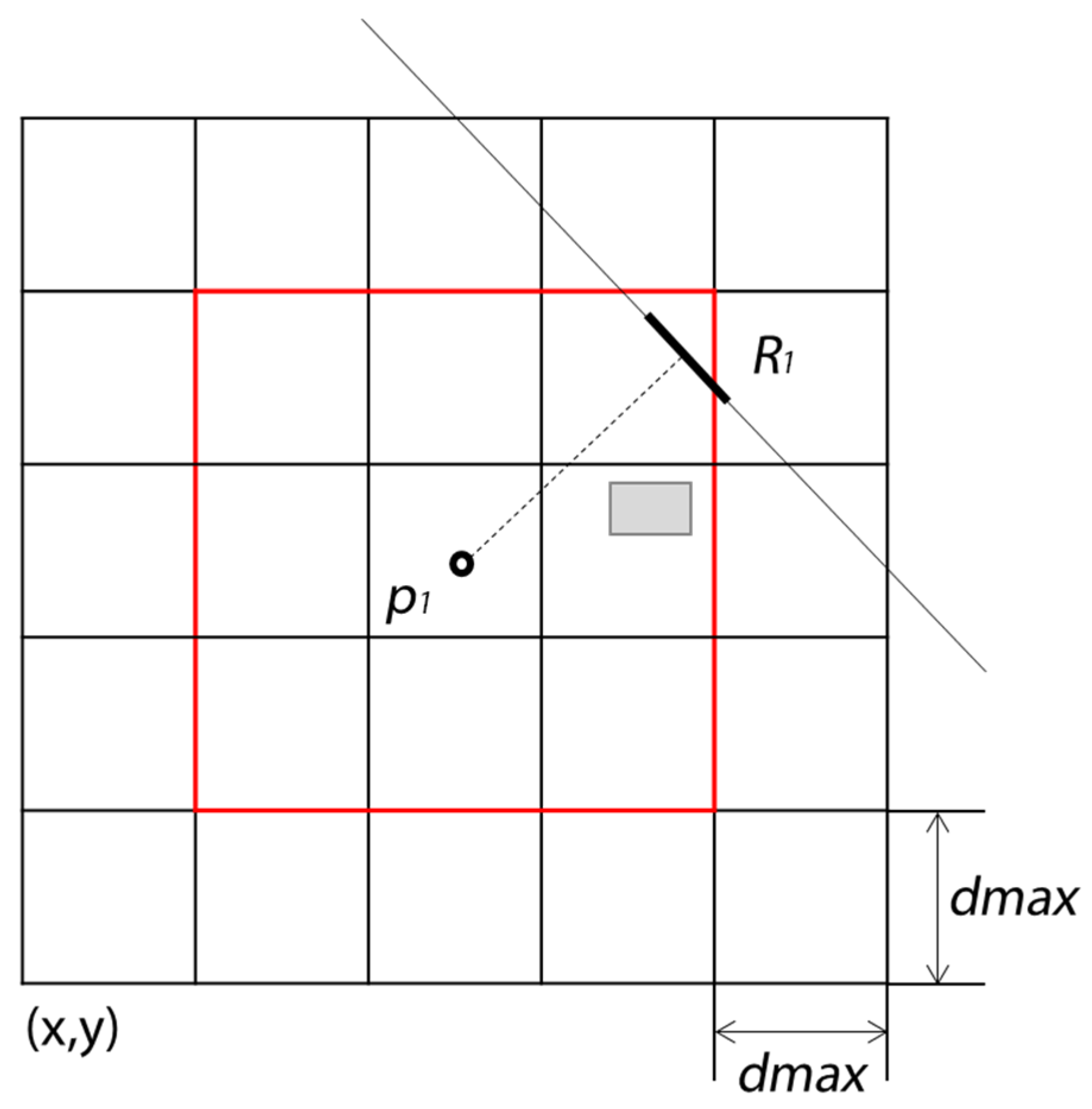
Furthermore, to optimize computational efficiency, a search radius threshold is introduced for receiving points, and a spatial grid is established for road segments and buildings. Considering noise attenuation with distance, when the distance from a sound source is large, the effect at the receiving point can be ignored. For example, if the propagation distance S is 200 m, the noise attenuation from road segment R1 to receiving point p1 is approximately 36 dBA, as obtained with Equation (16). Thus, we only need to consider the impact of road segments that are less than the distance threshold dmax. dmax can be modified depending on the noise mapping area and building density. Then, a spatial grid with a step length equal to the distance threshold in the area of noise mapping is established, as shown in Figure 6. First, the 2D grid indexes for receiving points, road segments and buildings are determined. If the index difference between a receiving point and a road segment or building is greater than 2 in any direction (which means that the distance between them is greater than the distance threshold, that is, outside the red box in Figure 6), the road segment or building is not used for estimation; otherwise, road segments and buildings are included. This can replace the distance measure and transform the global search into a local search. When there are large numbers of receiving points, it can significantly improve the retrieval efficiency.
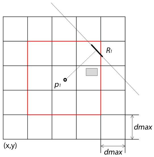
Figure 6.
Two-dimensional grid for receiving points, road segments and buildings.
After calculating the noise level at the receiving points, spatial interpolation is implemented to obtain the noise level in the whole region for noise mapping. In this case, model-based noise interpolation is different from noise interpolation at physical receiving points. The noise level at a receiving point in the model is based on the attenuation of noise propagation, and these points are densely distributed in the study region. In this article, bilinear spatial interpolation is used for noise mapping. Bilinear interpolation is a commonly used continuous surface interpolation method [35] that uses the values of the four nearest input elements to infer the output value. The output value is a weighted average of the four values and is adjusted based on the distance from the output element to each input element.
After noise interpolation, a traffic noise map is obtained from road surveillance video inputs. Road video is used to directly determine the traffic and environmental parameters required by the noise prediction model. By inputting road surveillance videos from different time periods, the traffic noise in the study area can be dynamically mapped.
4. Experiment
4.1. Data Collection
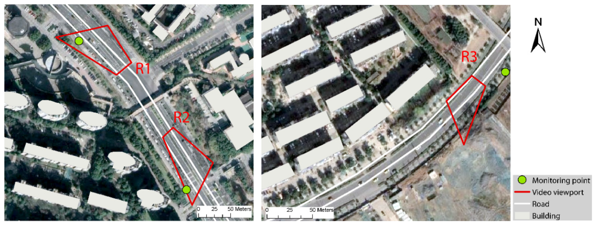
We selected Qixia District, Nanjing City, China, as the experimental area to test the proposed methods. Figure 7 shows an overview of the research area. The selected measurement time was the morning peak time period from 8:00 to 9:00. We collected one hour of surveillance video data during a flyover of three roads in two areas: R1 and R2 in area 1 and R3 in area 2. To reflect the complex traffic noise environment of cities as much as possible, both areas have high vegetation coverage, in which area 1 has higher buildings, including residential areas, schools and commercial areas, and area 2 has medium-height residential areas. We also monitored the noise levels along these roads at this time using AWA6228 noise monitoring equipment, which collected acoustic parameters, including LeqA, percentile levels, and standard deviation (SD).
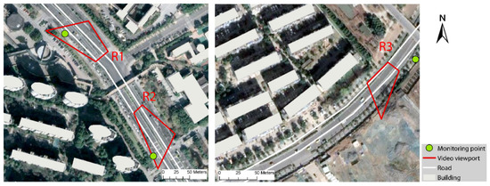
Figure 7.
Road network, buildings, video viewport and monitoring point in the experimental area.
The red boxes in Figure 7 are the viewports of the cameras. It describes the camera’s orientation and approximate coverage. The vector geographical data, including road networks and buildings, were downloaded in shapefile format from OpenStreetMap (www.openstreetmap.org (accessed on 1 November 2021)). The remote sensing image used for the selection of camera calibration control points was downloaded from Google Earth.
4.2. Results and Evaluation
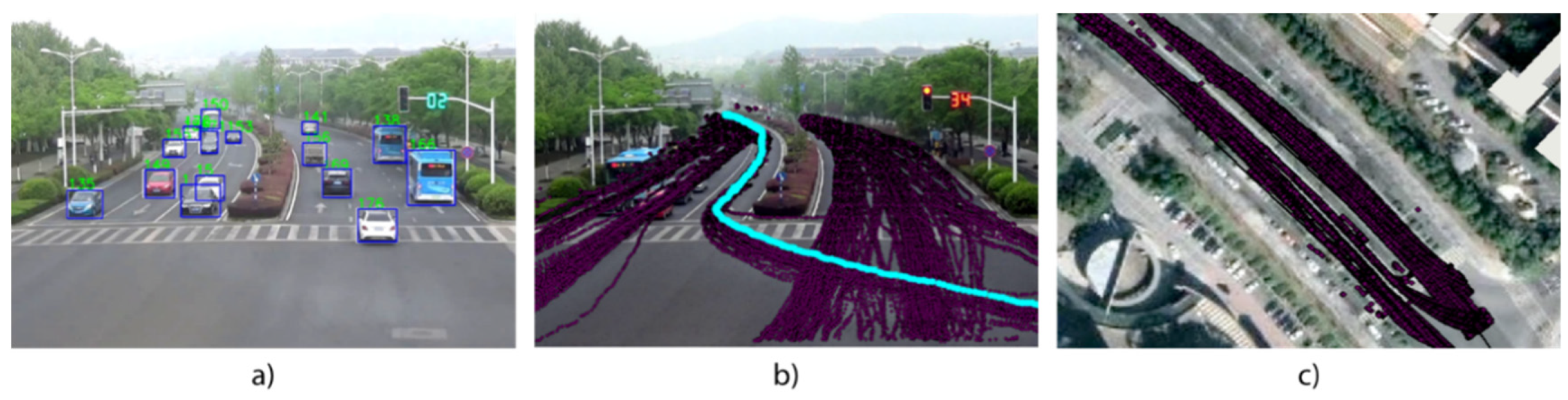
We implemented our method of video data processing with Python and the noise mapping model with C++. First, the traffic parameters and environmental parameters were extracted from the video. Figure 8 shows the traffic analysis for R1 based on road video data. Through vehicle detection, trajectory tracking and video calibration, the trajectories of all the vehicles that crossed the road were determined.

Figure 8.
Traffic analysis for road R1 based on road surveillance video data. (a) Vehicle detection in one frame of video, (b) vehicle trajectories and the highlighted points of one vehicle and (c) overlay of vehicle trajectories and a remote sensing image.
Table 3 shows the overall traffic statistics of the three roads. Notably, this is only used to compare the average traffic conditions of the three roads. As mentioned in Section 3.3.3, the specific noise calculation will segment the road and directly specify the traffic parameters of the road segments. Then, we compared the measured and simulated SPL (sound pressure level) at the monitoring points. The maximum absolute error was less than 2.4 dBA, and the average absolute error was 1.53 dBA. Among them, R3 has the highest traffic flow, large vehicle ratio and average speed, as well as its predicted and measured SPL. The comparison suggests that the model provides high-precision results.
Table 3.
Traffic parameters and sound pressure level in one hour for three roads.
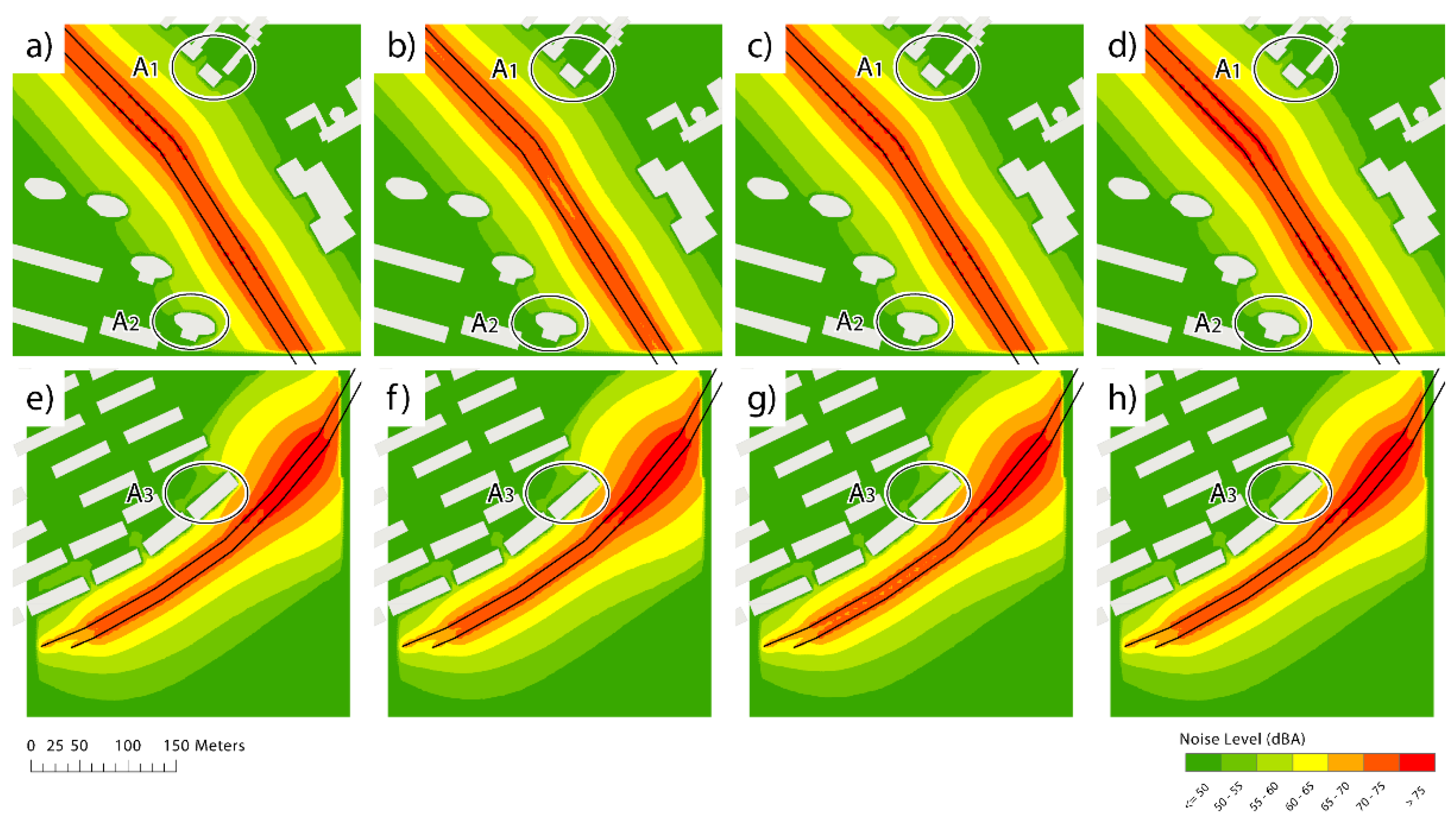
Moreover, we used the proposed model to map the dynamic noise level in the experimental area. We generated receiving points in a 3 × 3 m grid and performed bilinear spatial interpolation to obtain a noise map. Considering dynamic traffic flow and noise control, we generated dynamic noise maps at 15 min intervals to analyze the temporal and spatial distributions of the noise level in the experimental area. This time interval has been proven by some studies to be a good compromise between accuracy and efficiency [14]. The noise maps are shown in Figure 9. R1 and R2 are the northern and southern sections of the same road, respectively; thus, here, the overall noise level is calculated. If needed, because the traffic parameters are directly determined from road surveillance videos, the proposed method can be used to generate a noise map with a higher time resolution than 15 min.
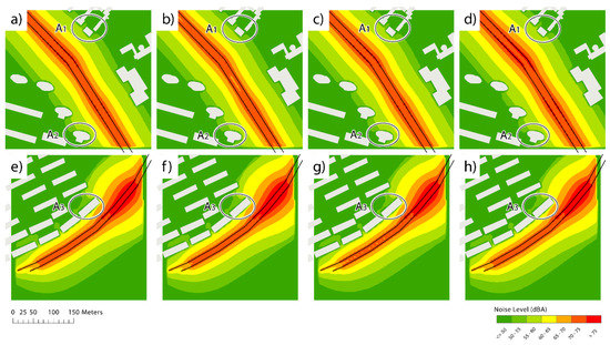
Figure 9.
Dynamic traffic mapping in the experimental area. (a–d) are the noise maps of R1 and R2 at 15 min intervals. (e–h) are the noise maps of R3 at 15 min intervals.
These noise maps, with high temporal and spatial resolutions, can be used to evaluate dynamic changes in the noise level at certain buildings or along specific road segments. The Environmental Quality Standard for Noise (GB 3096-2008, China) limits the noise level on both sides of the main roads in cities to 70 dBA and limits the noise level in residential areas to 55 dBA in the daytime. Surprisingly, noise levels on both sides of the three roads exceed these thresholds. Moreover, even after considering sound attenuation by the trees along roads, the noise levels at buildings on the outermost side of the road are still above the limits set for these areas.
Because traffic flows are dynamic, traffic noise changes significantly over short time intervals. For example, A1 is a school, but its noise level exceeds 55 dBA at three moments (a), (c) and (d). The noise levels of A2 and A3 located in the residential area all exceed 55 dBA at four moments. Overall, the noise level of area 2 is relatively stable, while the noise level of area 1 first decreases and then increases. The noise levels at some buildings along roads in these areas exceed the limit values, thus affecting the lives of residents and requiring further control.
5. Discussion
In this article, we proposed a road surveillance video-based method for dynamic traffic noise mapping. Here, we discuss the adaptability of the method from three perspectives: the noise prediction model, video calibration and object recognition accuracy. In this article, we propose a dynamic noise mapping model based on the RLS90 noise prediction model. Consistent with most noise prediction models, the proposed model includes a noise source model and a noise propagation model. In noise source models, specifying traffic parameters is essential. In this article, we calculated the average values of traffic parameters over a period of time. Some models, such as the CNOSSOS model, simulate the instantaneous traffic noise associated with a single vehicle [7]. The instantaneous noise level of a single vehicle is considered a function of the vehicle motion state and vehicle type. Additionally, the instantaneous speed and acceleration of each vehicle are considered. In this article, the method of extracting traffic parameters from video can be used to directly determine instantaneous vehicle speeds and types; therefore, this method is suitable for the simulation of noise from individual vehicles. In sound propagation modeling, most common noise prediction models perform sound propagation based on different mechanisms. For example, the RLS90 model is based on experience; conversely, there are some models, such as the CNOSSOS model, that use physics-based sound propagation models. However, the types of environmental factors considered in these models are similar [31]. These heterogeneous environmental factors that influence noise propagation are time-consuming and laborious to determine based on surveys. In this article, our method can adaptively specify these parameters in the noise model without actual measurement data.
Video calibration is essential for vehicle speed estimation and vegetation distribution determination. In this article, Zhang’s checkboard method is used to calibrate internal parameters, and the EPNP algorithm is used to calibrate external camera parameters. This approach based on the calibration checkerboard provides high accuracy and is suitable for cameras that do not move. In addition, camera self-calibration is another common camera calibration method. Notably, the relationship between two images of the surrounding environment is used to perform the calibration. Thus, this approach does not depend on a calibration reference object and is more flexible than the approach used in this paper. However, the solution process required with the flexible approach is complicated, and the result can be unstable [49]. Thus, the self-calibration method is most suitable when it is difficult to perform checkerboard calibration for each camera, such as when performing noise mapping for an entire city. In addition, due to the limitations of depth estimation with monocular cameras, only the planar distribution of vegetation can be extracted. Specifically, it is difficult to obtain the height and three-dimensional distribution of vegetation. Some recent studies have attempted to extract depth from monocular camera recordings [56]. In future studies, the extraction of vegetation height information from videos will be further explored.
Benefiting from deep learning and parallel computing, the proposed approach can identify and track vehicles in videos with high efficiency and precision. However, the object recognition accuracy is still affected by weather and the time of day. When conditions limit visibility, it remains challenging to use visible-light cameras to detect and track vehicles; notably, detection in severe weather and at night can be difficult. A recent study suggested that the matching of vehicle headlights and taillights to localize vehicle contours could improve the accuracy of vehicle detection and tracking at night [57]. Weather conditions also affect noise mapping, and further studies considering severe weather conditions and night vehicle detection methods are needed.
6. Conclusions and Outlook
Efficient dynamic traffic noise mapping is essential for urban noise management and building planning. However, due to the limitations of the dynamic acquisition of traffic parameters, dynamic noise mapping is still challenging. This paper presents a dynamic noise mapping method based on road surveillance video data. Unlike the existing methods that determine traffic parameters based on surveys, traffic model simulations and analyses of floating vehicle data, the proposed approach can be used to directly determine dynamic traffic parameters at the lane and segment levels. Thus, noise levels can be simulated at a high resolution. Moreover, environmental parameters that affect noise propagation, such as road materials, weather types, and vegetation types, can be determined from video and without other data. Through a comparison with noise levels measured by professional equipment, the noise map generated with the proposed method is characterized by high precision.
Although the proposed method offers some advantages over traditional methods, it still has several issues that require further investigation for quality improvement. First, the approach may be limited when mapping traffic noise over an entire city. Specifically, the proposed method would require road surveillance video data covering the entire urban road network. To efficiently map noise, it is necessary to optimize the efficiency of the applied algorithm and the computational resources of the noise model. Additionally, interactive noise mapping should be considered. Notably, with augmented reality or mixed reality, video data-driven noise maps can be visualized directly as noise isolines or as instantaneous noise levels for individual vehicles. It could be developed to allow users to better interact with the real world.
Author Contributions
Conceptualization, Yanjie Sun, Mingguang Wu, Xiaoyan Liu and Liangchen Zhou; Funding acquisition, Yanjie Sun, Mingguang Wu; Investigation, Yanjie Sun, Mingguang Wu, Xiaoyan Liu; Supervision, Mingguang Wu, Xiaoyan Liu and Liangchen Zhou; Visualization, Yanjie Sun; Writing—original draft Yanjie Sun; Writing—review and editing, Mingguang Wu; Software, Yanjie Sun, Xiaoyan Liu and Liangchen Zhou All authors have read and agreed to the published version of the manuscript.
Funding
This research study was funded by the National Natural Science Foundation of China: [41971417, 41571433] and the Postgraduate Research & Practice Innovation Program of Jiangsu Province [KYCX22_1575].
Institutional Review Board Statement
Not applicable.
Informed Consent Statement
Not applicable.
Data Availability Statement
Data sharing is not applicable to this article.
Conflicts of Interest
The authors declare no conflict of interest.
References
- European Commission. Noise in Europe 2014. 2014. Available online: https://www.eea.europa.eu/publications/noise-in-europe-2014 (accessed on 1 November 2021).
- Babisch, W. Updated exposure-response relationship between road traffic noise and coronary heart diseases: A meta-analysis. Noise Health 2014, 16, 1–9. [Google Scholar] [CrossRef]
- Basner, M.; McGuire, S. WHO Environmental Noise Guidelines for the European Region: A Systematic Review on Environmental Noise and Effects on Sleep. Int. J. Environ. Res. Public Health 2018, 15, 519. [Google Scholar] [CrossRef] [PubMed] [Green Version]
- Generaal, E.; Timmermans, E.J.; Dekkers, J.E.C.; Smit, J.H.; Penninx, B.W.J.H. Not urbanization level but socioeconomic, physical and social neighbourhood characteristics are associated with presence and severity of depressive and anxiety disorders. Psychol. Med. 2019, 49, 149–161. [Google Scholar] [CrossRef] [PubMed] [Green Version]
- WHO. Burden of Disease from Environmental Noise Quantification of Healthy Life Years Lost in Europe; WHO Regional Office for Europe and JCR European Commission: Copenhagen, Danish, 2011. [Google Scholar]
- Hammer, M.S.; Swinburn, T.K.; Neitzel, R.L. Environmental Noise Pollution in the United States: Developing an Effective Public Health Response. Environ. Health Perspect. 2014, 122, 115–119. [Google Scholar] [CrossRef] [PubMed] [Green Version]
- Kephalopoulos, S.; Paviotti, M.; Anfosso-Lédée, F. Common Noise Assessment Methods in EUROPE (CNOSSOS-EU); Publications Office of The European Union: Luxembourg, 2012; p. 180. [Google Scholar]
- Zhang, J.; Schomer, P.D.; Yeung, M.; Zhou, A.; Ming, H.; Chai, J.; Sun, L. A study of the effectiveness of the key environmental protection policies for road traffic noise control. J. Acoust. Soc. Am. 2012, 131, 3505. [Google Scholar] [CrossRef]
- De Kluijver, H.; Stoter, J. Noise mapping and GIS: Optimising quality and efficiency of noise effect studies. Comput. Environ. Urban Syst. 2003, 27, 85–102. [Google Scholar] [CrossRef] [Green Version]
- Asensio, C.; Pavon, I.; Ramos, C.; Lopez, J.M.; Pamies, Y.; Moreno, D.; de Arcas, G. Estimation of the noise emissions generated by a single vehicle while driving. Transp. Res. Part D Transp. Environ. 2021, 95, 102865. [Google Scholar] [CrossRef]
- Stoter, J.; Peters, R.; Commandeur, T.; Dukai, B.; Kumar, K.; Ledoux, H. Automated reconstruction of 3D input data for noise simulation. Comput. Environ. Urban Syst. 2020, 80, 101424. [Google Scholar] [CrossRef]
- Bastian-Monarca, N.A.; Suarez, E.; Arenas, J.P. Assessment of methods for simplified traffic noise mapping of small cities: Casework of the city of Valdivia, Chile. Sci. Total Environ. 2016, 550, 439–448. [Google Scholar] [CrossRef] [PubMed]
- Wei, W.; Van Renterghem, T.; De Coensel, B.; Botteldooren, D. Dynamic noise mapping: A map-based interpolation between noise measurements with high temporal resolution. Appl. Acoust. 2016, 101, 127–140. [Google Scholar] [CrossRef] [Green Version]
- Zambon, G.; Benocci, R.; Bisceglie, A.; Roman, H.E.; Bellucci, P. The LIFE DYNAMAP project: Towards a procedure for dynamic noise mapping in urban areas. Appl. Acoust. 2017, 124, 52–60. [Google Scholar] [CrossRef]
- Cai, M.; Yao, Y.; Wang, H. Urban Traffic Noise Maps under 3D Complex Building Environments on a Supercomputer. J. Adv. Transp. 2018, 2018, 7031418. [Google Scholar] [CrossRef] [Green Version]
- Bocher, E.; Guillaume, G.; Picaut, J.; Petit, G.; Fortin, N. NoiseModelling: An Open Source GIS Based Tool to Produce Environmental Noise Maps. ISPRS Int. J. Geo-Inf. 2019, 8, 130. [Google Scholar] [CrossRef] [Green Version]
- Can, A.; Picaut, J.; Ardouin, J.; Crepeaux, P.; Bocher, E.; Ecotiere, D.; Lagrange, M. CENSE Project: General overview. In Proceedings of the Euronoise 2021: European Congress on Noise Control Engineering, Madère, Portugal, 25 October 2021. [Google Scholar]
- Santhosh, K.K.; Dogra, D.P.; Roy, P.P. Anomaly Detection in Road Traffic Using Visual Surveillance: A Survey. ACM Comput. Surv. 2020, 53, 119. [Google Scholar] [CrossRef]
- Wang, W.; Yang, N.; Zhang, Y.; Wang, F.; Cao, T.; Eklund, P. A review of road extraction from remote sensing images. J. Traffic Transp. Eng. 2016, 3, 271–282. [Google Scholar] [CrossRef] [Green Version]
- Yan, Y.; Ryu, Y. Exploring Google Street View with deep learning for crop type mapping. ISPRS J. Photogramm. Remote Sens. 2021, 171, 278–296. [Google Scholar] [CrossRef]
- Lu, C.; Lin, D.; Jia, J.; Tang, C.K. Two-Class Weather Classification. IEEE Trans. Pattern Anal. Mach. Intell. 2017, 39, 2510–2524. [Google Scholar] [CrossRef] [PubMed]
- Ibrahim, M.R.; Haworth, J.; Cheng, T. WeatherNet: Recognising Weather and Visual Conditions from Street-Level Images Using Deep Residual Learning. ISPRS Int. J. Geo-Inf. 2019, 8, 549. [Google Scholar] [CrossRef] [Green Version]
- Guarnaccia, C. EAgLE: Equivalent Acoustic Level Estimator Proposal. Sensors 2020, 20, 701. [Google Scholar] [CrossRef] [PubMed] [Green Version]
- Murphy, E.; King, E.A. (Eds.) Chapter 4—Strategic Noise Mapping. In Environmental Noise Pollution, 2nd ed.; Elsevier: Boston, MA, USA, 2022; pp. 85–125. [Google Scholar]
- Lan, Z.; Cai, M. Dynamic traffic noise maps based on noise monitoring and traffic speed data. Transp. Res. Part D Transp. Environ. 2021, 94, 102796. [Google Scholar] [CrossRef]
- Banerjee, D.; Chakraborty, S.K.; Bhattacharyya, S.; Gangopadhyay, A. Appraisal and mapping the spatial-temporal distribution of urban road traffic noise. Int. J. Environ. Sci. Technol. 2009, 6, 325–335. [Google Scholar] [CrossRef] [Green Version]
- Mehdi, M.R.; Kim, M.; Seong, J.C.; Arsalan, M.H. Spatio-temporal patterns of road traffic noise pollution in Karachi, Pakistan. Environ. Int. 2011, 37, 97–104. [Google Scholar] [CrossRef] [PubMed]
- Can, A.; Dekoninck, L.; Botteldooren, D. Measurement network for urban noise assessment: Comparison of mobile measurements and spatial interpolation approaches. Appl. Acoust. 2014, 83, 32–39. [Google Scholar] [CrossRef] [Green Version]
- Murphy, E.; King, E.A. Smartphone-based noise mapping: Integrating sound level meter app data into the strategic noise mapping process. Sci. Total Environ. 2016, 562, 852–859. [Google Scholar] [CrossRef] [PubMed]
- Lesieur, A.; Mallet, V.; Aumond, P.; Can, A. Data assimilation for urban noise mapping with a meta-model. Appl. Acoust. 2021, 178, 107938. [Google Scholar] [CrossRef]
- Garg, N.; Maji, S. A critical review of principal traffic noise models: Strategies and implications. Environ. Impact Assess. Rev. 2014, 46, 68–81. [Google Scholar] [CrossRef]
- Barry, T.M.; Reagan, J.A. FHWA Highway Traffic Noise Prediction Model; Federal Highway Administration: Washington, DC, USA, 1978.
- Givargis, S.; Mahmoodi, M. Converting the UK calculation of road traffic noise (CORTN) to a model capable of calculating LAeq, 1h for the Tehran’s roads. Appl. Acoust. 2008, 69, 1108–1113. [Google Scholar] [CrossRef]
- RLS. Richtlinien für den Lärmschutzan Strassen; Der Bundesminister für Verkehr: Bonn, Germany, 1990. [Google Scholar]
- Seong, J.C.; Park, T.H.; Ko, J.H.; Chang, S.I.; Kim, M.; Holt, J.B.; Mehdi, M.R. Modeling of road traffic noise and estimated human exposure in Fulton County, Georgia, USA. Environ. Int. 2011, 37, 1336–1341. [Google Scholar] [CrossRef]
- Cai, M.; Zou, J.; Xie, J.; Ma, X. Road traffic noise mapping in Guangzhou using GIS and GPS. Appl. Acoust. 2015, 87, 94–102. [Google Scholar] [CrossRef]
- Bucur, V. (Ed.) Traffic Noise Abatement. In Urban Forest Acoustics; Springer: Berlin/Heidelberg, Germany, 2006; pp. 111–128. [Google Scholar]
- St-Aubin, P.; Saunier, N.; Miranda-Moreno, L. Large-scale automated proactive road safety analysis using video data. Transp. Res. Part C Emerg. Technol. 2015, 58, 363–379. [Google Scholar] [CrossRef]
- Espinosa, J.E.; Velastín, S.A.; Branch, J.W. Detection of Motorcycles in Urban Traffic Using Video Analysis: A Review. IEEE Trans. Intell. Transp. Syst. 2021, 22, 6115–6130. [Google Scholar] [CrossRef]
- Bochkovskiy, A.; Wang, C.-Y.; Liao, H.-Y.M. YOLOv4: Optimal Speed and Accuracy of Object Detection. arXiv 2020. [Google Scholar] [CrossRef]
- Soleimanitaleb, Z.; Keyvanrad, M.A.; Jafari, A. Object Tracking Methods: A Review. In Proceedings of the 2019 9th International Conference on Computer and Knowledge Engineering (ICCKE), Mashhad, Iran, 24–25 October 2019; pp. 282–288. [Google Scholar]
- Wojke, N.; Bewley, A.; Paulus, D. Simple online and realtime tracking with a deep association metric. In Proceedings of the 2017 IEEE International Conference on Image Processing (ICIP), Beijing, China, 17–20 September 2017; pp. 3645–3649. [Google Scholar]
- Zaitoun, N.M.; Aqel, M.J. Survey on Image Segmentation Techniques. Procedia Comput. Sci. 2015, 65, 797–806. [Google Scholar] [CrossRef] [Green Version]
- Minaee, S.; Boykov, Y.Y.; Porikli, F.; Plaza, A.J.; Kehtarnavaz, N.; Terzopoulos, D. Image Segmentation Using Deep Learning: A Survey. IEEE Trans. Pattern Anal. Mach. Intell. 2022, 44, 3523–3542. [Google Scholar] [CrossRef] [PubMed]
- Zhao, H.; Shi, J.; Qi, X.; Wang, X.; Jia, J. Pyramid Scene Parsing Network. In Proceedings of the 2017 IEEE Conference on Computer Vision and Pattern Recognition (CVPR), Honolulu, HI, USA, 21–26 July 2017; pp. 6230–6239. [Google Scholar]
- Liu, L.; Silva, E.A.; Wu, C.; Wang, H. A machine learning-based method for the large-scale evaluation of the qualities of the urban environment. Comput. Environ. Urban Syst. 2017, 65, 113–125. [Google Scholar] [CrossRef]
- Yang, C.; Li, Y.; Peng, B.; Cheng, Y.; Tong, L. Road Material Information Extraction Based on Multi-Feature Fusion of Remote Sensing Image. In Proceedings of the IGARSS 2019—2019 IEEE International Geoscience and Remote Sensing Symposium, Yokohama, Japan, 28 July–2 August 2019; pp. 3943–3946. [Google Scholar]
- Mountrakis, G.; Im, J.; Ogole, C. Support vector machines in remote sensing: A review. ISPRS J. Photogramm. Remote Sens. 2011, 66, 247–259. [Google Scholar] [CrossRef]
- Long, L.; Dongri, S. Review of Camera Calibration Algorithms. In Proceedings of the Advances in Computer Communication and Computational Sciences, Singapore, 22 May 2019; pp. 723–732. [Google Scholar]
- Zhang, Z. A flexible new technique for camera calibration. IEEE Trans. Pattern Anal. Mach. Intell. 2000, 22, 1330–1334. [Google Scholar] [CrossRef] [Green Version]
- Lepetit, V.; Moreno-Noguer, F.; Fua, P. EPnP: An Accurate O(n) Solution to the PnP Problem. Int. J. Comput. Vis. 2008, 81, 155. [Google Scholar] [CrossRef] [Green Version]
- ISO 9613-2:1996; Attenuation of sound during propagation outdoors. Part 2: General method of calculation. ISO: Geneva, Switzerland, 1996.
- Strigari, F.; Chudalla, M.; Bartolomaeus, W. Calculation of weather-corrected traffic noise immission levels on the basis of emission data and meteorological quantities. In Proceedings of the 7th Transport Research Arena TRA 2018, Vienna, Austria, 16–19 April 2018. [Google Scholar] [CrossRef]
- Huddart, L. The Use of Vegetation for Traffic Noise Screening; UK Transport and Road Research Laboratory: Crowthorne, UK, 1990.
- Roberts, C. Low frequency noise from transportation sources. In Proceedings of the 20th International Congress on Acoustics, Sydney, Australia, 23–27 August 2010; pp. 23–27. [Google Scholar]
- Gordon, A.; Li, H.; Jonschkowski, R.; Angelova, A. Depth From Videos in the Wild: Unsupervised Monocular Depth Learning From Unknown Cameras. In Proceedings of the 2019 IEEE/CVF International Conference on Computer Vision (ICCV), Seoul, Korea, 27 October–2 November 2019; pp. 8976–8985. [Google Scholar]
- Zhang, X.; Story, B.; Rajan, D. Night Time Vehicle Detection and Tracking by Fusing Vehicle Parts From Multiple Cameras. IEEE Trans. Intell. Transp. Syst. 2021, 23, 8136–8156. [Google Scholar] [CrossRef]


Publisher’s Note: MDPI stays neutral with regard to jurisdictional claims in published maps and institutional affiliations. |
© 2022 by the authors. Licensee MDPI, Basel, Switzerland. This article is an open access article distributed under the terms and conditions of the Creative Commons Attribution (CC BY) license (https://creativecommons.org/licenses/by/4.0/).