
Impacts of Urban Morphology on Seasonal Land Surface Temperatures: Comparing Grid- and Block-Based Approaches

1
Department of Urban Planning and Real Estate, College of Social Sciences, Chung-Ang University, Seoul 06974, Republic of Korea
2
Department of City and Regional Planning, The Ohio State University, Columbus, OH 43210, USA
*
Author to whom correspondence should be addressed.
ISPRS Int. J. Geo-Inf. 2023, 12(12), 482; https://doi.org/10.3390/ijgi12120482
Submission received: 31 July 2023
/
Revised: 12 September 2023
/
Accepted: 24 November 2023
/
Published: 28 November 2023
Abstract
:Highlights
- Urban 2-D and 3-D forms affect the built environment’s adaptability to surface heat and cold.
- Access to vegetation and water bodies helps moderate severe heat and cold across all seasons.
- Taller buildings are likely to reduce surface temperature in warm seasons due to shading.
- Older buildings with larger footprints are related to temperature increases across all seasons.
- Grid- and block-based approaches show comparable results in quadrant and regression analyses.
Abstract
Climate change is expected to result in increased occurrences of extreme weather events such as heat waves and cold spells. Urban planning responses are crucial for improving the capacity of cities and communities to deal with significant temperature variations across seasons. This study aims to investigate the relationship between urban temperature fluctuations and urban morphology throughout the four seasons. Through quadrant and statistical analyses, built-environment factors are identified that moderate or exacerbate seasonal land surface temperatures (LSTs). The focus is on Seoul, South Korea, as a case study, and seasonal LST values are calculated at both the grid (100 m × 100 m) and street block levels, incorporating factors such as vegetation density, land use patterns, albedo, two- and three-dimensional building forms, and gravity indices for large forests and water bodies. The quadrant analysis reveals a spatial segregation between areas demonstrating high LST adaptability (cooler summers and warmer winters) and those displaying LST vulnerability (hotter summers and colder winters), with significant differences in vegetation and building forms. Spatial regression analyses demonstrate that higher vegetation density and proximity to water bodies play key roles in moderating LSTs, leading to cooler summers and warmer winters. Building characteristics have a constant impact on LSTs across all seasons: horizontal expansion increases the LST, while vertical expansion reduces the LST. These findings are consistent for both grid- and block-level analyses. This study emphasizes the flexible role of the natural environment in moderating temperatures.
1. Introduction
Global warming and climate change are leading to an increase in extreme weather events worldwide. New climate norms include the largest number of droughts since 1974, an early summer heat wave occurring in spring, and a strong cold shock in fall [1,2]. These severe weather events closely impact human health and well-being. According to the World Health Organization [3], climate change is expected to cause approximately 250,000 deaths per year from 2030 to 2050. With continued urbanization, the temperature rise in urban centers will likely accelerate, necessitating appropriate mitigation measures and environmental adaptation strategies.
Atmospheric temperature (AT) and land surface temperature (LST) are often used in urban temperature research, but the latter is more clearly affected by the spatial and temporal traits of micro- and meso-scale urban morphology and surface composition [4]. Therefore, many studies have used LST as an indicator of thermal variability in response to urban changes. Urban structures, such as buildings and roads, significantly contribute to urban warming [5,6]. Identifying and analyzing the components of a city and their varying impacts on thermal conditions are fundamental steps in sustainable urban design [7,8,9]. Urban form analysis can also assess the adaptability of cities to extreme temperatures [10,11]. Thus, understanding urban form factors closely related to LST variations over space and seasons is crucial for urban management.
Urban LST is influenced by multiple factors, ranging from land cover materials to horizontal and vertical urban geometry, and their effects may depend on the seasonal and spatial context [12,13]. For example, urban forests and woods are beneficial for urban cooling, owing to active evapotranspiration and shading, but their impacts in cold months are less understood. Similarly, urban water bodies, such as lakes and ponds, have surface temperatures lower than those of their surroundings in summer, but the thermal impact of large stretching rivers is less understood [14,15,16]. The seasonal effects of conserving and restoring urban blue spaces need to be better understood. Additionally, the correlation between LST and its associated factors has generally been examined on a grid system, but research on the suitability of using block-based data aggregation to explain LST variability is lacking [17]. This study aims to identify the impacts of multi-dimensional urban form and spatial indicators on seasonal LST using two data aggregation systems—grid and block units—and to explore desirable urban forms that can be flexibly adapted to different seasons.
This paper has the following research objectives, focusing on Seoul, South Korea, as the study area: (1) clarifying how each seasonal LST pattern is influenced by different urban morphology factors, including land-use/land-cover (LULC) characteristics, 2-D/3-D form of man-made structures, and proximity to green and blue spaces; (2) identifying which urban areas have moderate summer and winter LSTs as compared to others by classifying them into four quadrants of temperature; and (3) exploring the impact of spatial unit choice on understanding factors affecting LST by applying spatial regression analysis to both grid- and block-based datasets.
The paper is organized as follows: Section 2 presents a review of the literature on urban morphological and natural factors related to LST. Section 3 describes the study areas and data processing. Section 4 describes the statistical methodology, including quadrant and regression analyses. The results are presented in Section 5 and discussed in Section 6. Section 7 concludes this paper.
2. Literature Review
Urban LST results from various natural and built environmental factors, including solar radiation, meteorological conditions, surface biophysical composition, landscape characteristics, and building form [18,19]. Surface biophysical composition refers to the land cover, such as tall/short vegetation, asphalt, concrete, steel, brick, bare soil, and water. Natural green and blue spaces rarely experience a large temperature change, as they act as temperature moderators across seasons [16,20]. Converting natural land cover into urbanized impervious surfaces significantly increases LST in warm seasons, primarily because of the removal of evapotranspiration cooling by vegetation and water bodies and the increase in low-albedo materials such as buildings and roads [21,22,23]. Surface albedo significantly influences LST by altering solar radiation absorption [24,25]. Low-albedo urban features absorb and retain a significant amount of solar radiation, instead of reflecting it, and release the heat slowly, exacerbating the urban heat island effect [13,22].
Land cover composition is often quantified using remotely sensed spectral indices, including the Normalized Difference Vegetation Index (NDVI), the Normalized Difference Built-up Index (NDBI), and the Modified Normalized Difference Water Index (MNDWI). These indices are consistently and significantly correlated with LST across seasons [26,27,28]. Dense vegetation helps regulate LST, reducing LST in summer while increasing it in winter [20]. Built-up surfaces in cities can reduce the cooling effect of vegetation’s evapotranspiration, intensifying urban warming [26]. MNDWI (percent water content) is negatively correlated with LST [21,27,29]. Another approach to quantifying land cover composition is calculating the proportions and spatial arrangements of LULC types using landscape metrics [30]. While metrics summarize distinct LULC patterns, individual metrics’ effects are not well understood because they are calculated based on different land cover classification schemes and grid sizes [19,23,31]. The percentages and mix of distinct LULC types may provide a comparable control for LST effects and facilitate interpretation.
Building form significantly impacts spatial LST distribution through vertical form, horizontal spacing, and urban canyon characteristics, affecting thermal mass, shadow casting, wind swirling, and waste heat release [32,33,34,35]. Studies on building form’s effects on seasonal LST find that horizontal building densification, often measured by urban compactness, building coverage ratio (BCR), and surface-to-volume ratio, increases LST, while vertical densification, often proxied by building height (BH), decreases it, and these effects remain stable across seasons [18,36,37,38]. Taller buildings can reduce summertime LST by casting shadows on adjacent buildings and grounds [35,39,40]. The transition point for the BH’s impact on LST occurs around 10 m, above which the BH reduces LST due to increased shade [18]. However, there are mixed findings for other building indices, such as the Sky View Factor (SVF), frontal area index, floor area ratio, and building coverage ratio, whose nonlinear effects may vary by season and location [5,13,18,33].
The LST pattern of a given area is influenced by the LST of adjacent areas due to air convection and wind flow, resulting in the LST values in close proximity being spatially autocorrelated [41,42,43]. However, this spatial spillover has rarely been considered in modeling seasonal LST variations. Another source of LST autocorrelation is where large natural areas can influence neighboring areas by spreading additional cooling or warming effects [14,16,44,45,46]. Investigating the cooling effect of river bodies, Cai et al. [36] observe that the relationship between building form and seasonal LST becomes stronger as the distance to the closest river corridors increases. Hu et al. [33] utilize a gravity index for each LST grid cell based on the distance to and area of nearby parks, finding that larger park areas in closer proximity result in a stronger cooling effect, albeit significant only in spring and summer. Few studies account for the area and proximity of large natural zones such as forests and rivers simultaneously in modeling seasonal LST. Whether thermal propagation from those natural reserves to urban settlements is positive or not remains underexplored.
The spatial unit of analysis used to quantify urban form varies across studies. Previous investigations of the relationship between seasonal LST and urban factors have primarily used data aggregated over uniform grid cells [27]. Some studies have tested the effect of the grid scale on LST estimation [18,20,21,37,38], with different conclusions regarding the optimal grid size. While this grid processing is natural due to the availability of satellite thermal infrared observations in grid format, it requires truncating the spatially continuous urban form into discrete pieces to align with the grid cells [47]. Urban planning and development occur at the site or block scale, typically encompassing street segments and natural corridors. A street block represents a homogeneous area in terms of buildings and LULC but varies in size [48]. Research exploring whether block-level data aggregation and modeling of LST produce results consistent with conventional grid-based analysis is scarce.
To address the above gaps, this study explores the impacts of three groups of urban form factors on seasonal LST by comparing both grid- and street block-based data aggregations. The urban form factors considered include NDVI, surface albedo, land-use proportions and diversity, 2-D/3-D building form, and proximity to natural zones. Their individual effects are estimated using spatial models that control for spatial autocorrelation. Additionally, this study examines whether there are significant similarities and dissimilarities among areas with favorable thermal conditions, mitigating summer heat and winter cold, and those with the least favorable thermal conditions.
3. Study Area and Data
3.1. Study Area
The study area is the City of Seoul, the capital of South Korea. Seoul serves as the epicenter of commercial and business activities and is intertwined with densely developed and diverse residential districts. With an area of 605.2 km2, Seoul represents 0.6% of the national territory, yet it accommodates approximately 17% of the nation’s total population. The city’s metropolitan area is recognized as one of the most densely populated regions globally, ranked ninth by population [49]. Geographically, the city is situated in the northwestern part of South Korea, with the Han River flowing through the city from east to west (Figure 1). Surrounded by mountains, Seoul lies in a basin, with several smaller tributaries feeding into the Han River. The city features numerous bridges that facilitate transportation between different areas. Seoul experiences four distinct seasons, including hot and humid summers, with temperatures occasionally exceeding 30 °C, and cold winters, with average temperatures falling below freezing and with intermittent snowfall. Given these diverse conditions, Seoul presents an ideal case study to explore the influence of complex urban built-up and natural form characteristics on seasonal thermal environments, contributing to the geographic diversity of empirical LST research.
3.2. Data Sources and Processing
3.2.1. Grid Cells Versus Street Blocks
LST exhibits spatial variations influenced by local physical characteristics, and various spatial units are employed to delineate these locations and process local attributes. Geospatial data are commonly distributed in raster or lattice (areal vector) format. Raster-grid-based analysis has been extensively utilized for LST data analysis, owing to its efficiency in handling large-scale continuous geospatial information, particularly since LST images are initially generated as collections of image pixels.
Despite its advantages, grid-based data processing involves dividing physical elements into uniformly sized grid cells, leading to artificial truncation that may introduce biases in LST analyses. The grid size is determined by sensor capabilities rather than scientific rationale. Thus, this study explores whether a lattice-based analysis yields different results compared to the grid-based approach (Figure 2). Urban landscapes are divided into homogenous blocks by streets and roads, creating coherent spatial units in terms of land use and buildings. These street-enclosed blocks likely represent homogeneous neighborhoods governed by similar land-use regulations, including design codes and caps for BCR and floor area ratio (FAR). Consequently, we also utilize street-enclosed neighborhood blocks as alternative spatial units for LST analysis and compare the results obtained from both approaches. The Ministry of the Interior and Safety has recently developed a street block unit system known as the state basic district (SBD), where boundaries are delineated based primarily on transportation and river networks. In this study, we select and compare the grid and street blocks as spatial units of analysis.
3.2.2. Land Surface Temperatures
Seasonal LST values across Seoul were extracted from Landsat 8 Thermal Infrared Sensors Collection-2 Level-2 products, featuring a 30 m spatial resolution, accessed through Earth Explorer, which is the data distribution platform operated by the United States Geological Survey. This dataset comprises atmospherically corrected surface reflectance and surface temperature values derived from Level-1 inputs meeting specific technical criteria to ensure scientific validity. Remotely sensed LST data allow for spatially continuous analysis and exhibit a strong correlation with AT measures, which are typically available from only a limited number of meteorological stations. Theoretically, a new Landsat 8 image is available every 16 days, but many of them are unusable because of clouds. Three criteria are considered for LST image selection. First, the image must be dated between 2014 and 2022, because 2-D/3-D building information is available as of 2014. Second, there must be at least one cloud-free image for a specific time in the middle of each season. The only satisfactory year was 2017. Lastly, the year and specific day of image acquisition needs to be free of extreme weather [50]. As a result, one image for each season in 2017 was selected considering data availability and meteorological conditions (Figure 3). According to the World Meteorological Organization (WMO), 2017 was when neither El Nino nor La Nina was present; ENSO-neutral conditions continued during the year 2017 [51]. Table 1 presents the date and time of data collection.
Seoul features extensive nature preserves, with approximately 13% of the city’s area covered by public waters, such as rivers and tributaries, and an additional 25.3% covered by forests and woods. In total, approximately 38% of the city comprises uninhabited natural reserves. As these areas lack urban built-up activities and land uses, they are excluded from subsequent analyses to avoid zero-inflation issues in the dataset. Moreover, the LST patterns of natural features differ significantly from those of urbanized areas. Hence, this study focuses exclusively on the built-up morphology of urban areas and its impact on LST. For subsequent analyses, those grid cells and street blocks that have significant overlap with natural reserves (i.e., rivers and forests) are removed. More precisely, grid cells (blocks) where more than 5% of the area is water or more than 30% is forest are removed (since vegetation density within the area is accounted for using NDVI, a higher threshold is applied to forest proportions). In addition, those grid cells that have no overlap with blocks are dropped for consistency in areal coverage between grid- and block-based analyses.
To address the spillover effects of nearby natural features on the LST of adjacent urban areas, the final dataset includes variables quantifying the proximity to forests, rivers, small green spaces, and water bodies as distinct land-use types.
For the grid-based analysis, the LST cells with a 30 m resolution were resampled to 100 m by 100 m, using bilinear interpolation in ArcGIS to align with building geometry and density information, where the smallest unit is a 100 m grid. On the other hand, for the block-level analysis, the mean LST values were calculated for each individual block. A total of 34,135 grid cells and 4553 street blocks are considered in this study.
4. Methodology
4.1. Built-Environment Variables
4.1.1. NDVI and Albedo
The NDVI is a widely used indicator of vegetation density or photosynthetic activity, and it is calculated as follows:
where RED and NIR are the surface reflectance in the red and near-infrared bands, respectively [52]. These surface reflectance (SR) values are obtained from Landsat 8 data at a 30 m resolution, and NDVI values are calculated for each of the four seasons. NDVI ranges from −1 to 1, with higher values indicating higher vegetation density and health and lower values indicating impervious land with limited vegetation or water content. The NDVI values in this study are min–max transformed to the 0–1 range.
Surface albedo quantifies the extent to which a surface reflects solar radiation and is expressed as a percentage ranging from 0 (indicating no reflection) to 100 (indicating complete reflection). Surfaces with high albedo values include white materials like snow and clouds, which remain cooler due to their ability to reflect a significant portion of incoming solar radiation. Conversely, darker surfaces, such as asphalt, dark trees, and soil, exhibit low albedo values and tend to absorb a larger portion of solar energy, leading to increased warmth. Given the influence of surface albedo on surface temperature, it is essential to account for this characteristic when modeling LSTs. The calculation of albedo is based on Landsat SR bands, utilizing the formula proposed by Liang [53]:
where SWIR1 and SWIR2 represent short-wave infrared in different bandwidths. Both seasonal NDVI and surface albedo values are aggregated at the 100 m grid level and the block level, respectively.
4.1.2. Land Uses and Buildings
Land use classification data available at the land parcel level in vector form are downloaded from the Korean Ministry of Environment’s website, Environmental Geographic Information Service (EGIS) [54]. The classification is conducted via manual digitization based on very-high-resolution orthorectified aerial images (0.25 m/pixel). In this study, seven land-use categories are considered—residential, commercial, industrial, cultural and recreational, transport, public, and others (non-urban uses)—and their proportions within each grid cell and block are interfaced with seasonal LST values. In addition, the entropy index is used as a metric to measure the level of land-use diversity, with the following:
where is the percentage of land use type j in the grid cell (block) and k is the total number of land-use types considered. It ranges from 0 to 1, with higher values indicating a balanced mix of different land uses.
GIS data were gathered on various building characteristics, including the density of buildings, the percentage of aged buildings, BCR, total floor area (TFA), FAR, and BH. The data were obtained from the National Geographic Information Institute (NGII), which provides building information in two different data formats: grid cells of varying sizes and lattice formats encompassing state basic districts (SBDs), census tracts, zip code areas, villages, and municipalities. To ensure data consistency, the finest spatial unit from each format is selected for data acquisition, resulting in a grid size of 100 m and the use of SBDs. While individual building information would have been valuable, it is unfortunately unavailable. Therefore, building form indicators, as processed by the NGII [55], are retained along with land-use proportions and land-use diversity variables for subsequent statistical analyses. This study employs six building indicators, with three related to two-dimensional aspects and the remaining three to three-dimensional aspects. Table 2 lists and describes all the variables used in the analysis.
4.1.3. Gravity Index
Two gravity indices are calculated for urban forests and for water bodies at the grid and block levels. The gravity index measures the distance-decay impacts of urban forests and water bodies on LST [21,33]. First, a 1000 m buffer is constructed around the centroid of any grid cell or street block i, and the areas of urban forests and water bodies are converted into points with intervals of 30 m in GIS. The cooling effects of forests and water bodies tend to decrease as the distance from their boundaries increases. However, there is little consensus regarding the distance at which these cooling effects fade out. Regarding urban parks, Hu et al. [33] use a buffer distance of 1500 m to capture the cooling effects of urban parks in Beijing. Geng et al. [56] select a buffer threshold of 1000 m surrounding each urban park to study their LST impact. Lin et al. [57] find that cooling effects extend as much as 840 m away from urban parks in Beijing. Xiao et al. [58] use a buffer radius of 500 m to capture the cooling intensity of parks in Nanjing. As for water bodies, Cai et al. [36] find that the cooling effect of water bodies can reach 1000 m (horizontal distance). This study uses the buffer radius values common to the literature on urban parks and water bodies—1000 m. Let be the buffer of centroid i, j be a point within this buffer, be the distance between the centroid i and point j, be the area, either forests or waters, represented by point j (900 m2), and α be a positive exponent; then, the gravity index is defined as follows:
This gravity index accounts for the fact that the influence of forests on LST may be reduced by the distances to these forest areas, and the effect of distance is discounted by the exponent α. Higher α values decrease the importance of farther-away forests (waters) while increasing the influence of nearby ones. Several α values (1.0, 1.5, 2.0, 2.5, and 3.0) were tested, with α = 1.5 providing the best statistical fit.
4.2. Statistical Analyses
4.2.1. Quadrant Analysis
A four-quadrant analysis is a simple but useful tool to assess the current situation and aid in decision-making [59,60]. The quadrant analysis in this study involves the division of grid cells and blocks into four categories based on the intersection of summer LST on the x-axis and winter LST on the y-axis (Figure 4). These “temperature quadrants” are characterized as follows: the first quadrant exhibits hotter LST in summer and warmer LST in winter compared to the other areas; the second quadrant represents the most desirable condition, with cooler summer LST and warmer winter LST; the third quadrant contains cooler LSTs in both summer and winter; and the fourth quadrant indicates the worst case, with higher temperatures in summer and colder temperatures in winter. The spatial distributions of these quadrants across Seoul are explored to assess whether there are significant statistical dissimilarities among them in terms of vegetation and built-up morphology. To achieve this, one-way analysis of variance (ANOVA) and post hoc tests are employed to determine specific pairs of quadrants with significant differences in mean values.
4.2.2. Regression Analysis
The regression analysis is conducted to estimate the relationship between LST and the urban morphological attributes over the four seasons. Applying regression models to a large LST dataset allows for identifying the independent, disaggregated effect of each explanatory variable while controlling for the influence of the other variables and geographically neighboring areas.
Different forms of regression are considered: the ordinary least square model (OLS), the spatial lag model (SLM), the spatial error model (SEM), and the general spatial model (GSM), incorporating SLM and SEM. Each of these models is estimated in a sequence suggested by LeSage [61] and Anselin [62]. The LST in each cell is likely to be closely related to LST values in nearby cells, because of thermal advection and air circulation. This spatial autocorrelation (SA) can be accounted for in spatial regression models. The basic specification of the OLS model is as follows:
where Y (i.e., LST) is the column vector of the dependent variable, X is a matrix of the explanatory variables, is a vector of coefficients, and is a vector of normally and independently distributed random errors. The Moran’s I test is used to test whether SA exists among OLS residuals. If so, spatial regression models are needed. The SLM assumes that SA exists in the distribution of the dependent variable, with the following:
where is the spatial lag factor, a measure of the SA, W is a spatial weight matrix defined by spatial contiguity of the first order and is in a row-stochastic form, and is the vector of the spatially lagged dependent variable. The SEM assumes that only the error terms are spatially autocorrelated, with the following:
where is a measure of the SA. The GSM assumes that both the dependent variable and the error terms are spatially autocorrelated, with the following:
where measures the magnitude of the influence of the adjacent LST values on the central cell LST and represents the effects of the unobserved variables nearby that are captured by the error term. A set of statistical diagnostics for the assessment of model misspecification due to SA has been developed by Anselin [62,63] based on the Lagrange multiplier (LM) principle and used in many prior studies [20,35,64,65,66,67]. The most appropriate model is determined based on three statistical criteria: Moran’s I, the Lagrange multiplier (LM), and robust LM tests. The LM test assesses whether both lambda in the spatial error term (λWu) for the effect of unobserved variables and rho in the spatial lag term (ρWY) for the SA of LST are statistically significant. To determine the relative fit of SEM and SLM, the robust LM test is applied. Robust LM error assesses whether the spatial error term remains statistically significant (λ ≠ 0) when the spatial lag term is included in the model (ρ ≠ 0), while robust LM lag assesses whether it is still appropriate to include the spatial lag term when the spatial error term is controlled for. To select and implement spatial regression models, two software packages are used: Matlab (R2023b) and GeoDa (1.22). The k-nearest-neighbor criterion is adopted for the spatial weight matrix, which defines adjacency between areas based on their distance.
5. Results
5.1. Descriptive Statistics
This study investigates the relationships between LST and urban built-up morphological traits at both the grid cell and street block levels, and one of the traits is the proximity to urban forests and rivers. To calculate the gravity indices for urban forests and rivers, respectively, at the grid and block levels, several α values (1.0, 1.5, 2.0, 2.5, and 3.0) were tested, with α = 1.5 providing the best statistical fit. The mapping of the gravity indices for urban forests (GIUF) and for water bodies (GIWB) is presented in Figure 5 and Figure 6. Descriptive statistics for all the explanatory variables for the grid and block systems are presented in Table 3 and Table 4.
5.2. Quadrant Analysis
Based on the average summer and winter LSTs (37.4 °C and −2.36 °C for grid cells, and 37.8 °C and −2.5 °C for blocks, respectively), grid cells and blocks are categorized into four quadrants (see Figure 4). The results of the summer and winter LST quadrant analysis, presented in Table 5, reveal that Q1 is the most prevalent type, encompassing the largest number of grid cells (33.9%) and blocks (36.6%), followed by Q3, which includes 28.8% of the grid cells and 30.0% of the street blocks. This indicates that approximately 63% to 66% of the entire city consistently experiences warmer LST in summer and colder LST in winter, as compared to other areas. Areas with relatively cooler summer and warmer winter temperatures (Q2) account for approximately 16.2% at the grid level and 15.1% at the block level. Meanwhile, areas with the least favorable LST conditions (Q4), warmer in summer and colder in winter, account for approximately 21.1% of the area at the grid level and 18.3% at the block level.
The spatial distribution of these four quadrants across Seoul’s 25 local districts shows significant clustering, with spatial disparities among the districts in terms of quadrant proportions (Figure 7). Some districts located northeast and southwest of Seoul exhibit disproportionately larger numbers of Q4 units, indicating a large contiguous cluster of grid cells and blocks with unfavorable LST conditions. On the other hand, various other districts located southeast of Seoul show very few traces of Q4 units. The three districts with the fewest number of Q4 units consist of socioeconomically well-to-do communities and high-end commercial centers, which are typically characterized by higher property values and well-maintained green infrastructure. These districts predominantly comprise Q2, Q3, and Q1 units.
Notably, Q2 units (cooler summer and warmer winter) tend to be located more along the rivers and streams, particularly the Han River that cuts through Seoul. Q3 units (cooler summer and colder winter) also exhibit a similar spatial pattern, being situated close to water bodies, but they are more densely clustered near urban forests and mountains north and northwest of Seoul. Additionally, some districts to the east and northwest of Seoul are predominantly composed of Q1 and Q4 units, indicating vulnerable thermal conditions in summer and winter. These areas coincide with large local clusters of affordable residential areas in Seoul, indicating an inequitable social distribution of summer heat and winter cold.
The comparison of the mean values of the urban form variables, including NDVI, building form indicators, and proximity to forests and water bodies, provides further insights into the characteristics of each quadrant (Table 5). Q2 exhibits the highest vegetation density in both summer and winter. It also has greater access to large water bodies in its vicinity when compared to the other quadrants, as well as moderate access to urban forests nearby. Q3 ranks second to Q2 in terms of vegetation density in both seasons and access to water bodies, but it excels in its proximity to urban forests. It appears that urban natural elements such as greenery and waterfront areas are closely associated with pleasant changes in LSTs in summer and winter.
Furthermore, the quadrants significantly differ in terms of building form and geometry. Q2 and Q3 have lower building densities, percentages of aged buildings, and BCRs than Q1 and Q4, but they boast higher or comparable average BHs and volumes (TFAs). This indicates that Q1 and Q4 include areas with high population density, which are characterized by mid-to-low-rise buildings situated close to one another and located farther away from rivers and forests within the city. On the other hand, Q2 and Q3 areas exhibit more spaced-out, taller buildings and have better access to urban green spaces and water features.
5.3. Regression Analyses of LST
5.3.1. Model Selection
Multivariate regression models are employed to investigate the impact of individual urban built-up form variables on seasonal LST variations. Given the observed spatial correlation between LST and urban form indicators, spatial regression models are explored. Moran’s I statistics indicate significant SA in the error term of the OLS models for both grid- and block-level analyses across all four seasons (Table 6). This points to the necessity of controlling for spatial autocorrelation. The LM test confirms that both lambda in the spatial error term (λWu) and rho in the spatial lag term (ρWY) are statistically significant (λ ≠ 0 and ρ ≠ 0), indicating the suitability of SEM and SLM over OLS at both grid and block scales in all seasons. The robust LM test of the four-season LST models at the grid and block levels shows that both robust LM error and lag statistics are significant, with the former being higher than the latter in all cases. This suggests that the GSM that integrates both error and lag terms is preferred. Consequently, subsequent regression analysis of seasonal LST at grid and block scales is conducted using the GSM.
5.3.2. Model Estimation: Grid Level
The GSM is employed to explain LST variations across all four seasons, utilizing both grid- and block-level databases. This regression analysis allows for a statistical understanding of an anticipated change in seasonal LST in response to a change in each explanatory variable. The spatial error and lag terms demonstrate statistical significance with substantial coefficients, affirming the suitability of spatial regression over OLS. The results indicate that the model for summer LST is well explained by the current set of variables, as indicated by its highest R2 value, with almost all explanatory variables being statistically significant (Table 7). In contrast, the winter LST model shows the lowest R2 value, implying that winter temperatures are more challenging to explain based on urban built-up form indicators, such as vegetation, land use, building characteristics, and proximity to nature. The variance in LST is much smaller in winter than in other seasons, indicating a stronger association between urban form and heat rather than cold (Table 3 and Table 4). Summer corresponds to the most substantial impact from urban natural and artificial environments.
The results of the grid-based GSM estimation reveal that two urban built-up form factors play a crucial role in the city’s adaptive capacity to temperature changes across the four seasons: vegetation density, represented by NDVI, and proximity to water bodies, represented by the gravity index for rivers and streams (GIWB) (Table 7). These two variables exhibit opposite coefficient directions between summer and other seasons. Higher vegetation density leads to cooler summer and warmer winter LSTs. A higher winter NDVI, suggesting a higher density of evergreen trees and lawns, increases LST significantly. Additionally, closer proximity to water bodies reduces LSTs in summer and spring but increases LSTs in winter and fall. This indicates that areas located near rivers, streams, and other water bodies are more likely to experience lower temperatures in summer and warmer temperatures in winter compared to areas without such proximity (within 1 km). Careful management of vegetation health and water content in urban areas has considerable potential to mitigate temperature extremes and naturally regulate heat and cold. However, proximity to urban forests and mountains consistently decreases LSTs across all seasons. Unlike urban greenery, hilly mountains covered by forests block sunlight and trap cold air near the ground, leading to overall colder conditions. Moreover, forests contribute to increased humidity due to evaporation, intensifying the perception of cold temperatures. Seoul’s urban forests, situated at higher altitudes, lead to temperature drops both within the forests and in adjacent areas owing to atmospheric inversion.
The effects of the other urban form variables on LST remain consistent across all seasons. Most urban land-use types increase LSTs in every season. Industrial and cultural/recreational uses tend to have a stronger impact on increasing LST, which is likely due to the expansive building interior spaces required for industrial production and recreational facilities. Residential and commercial uses, as well as roads and parking lots, also contribute to elevating LSTs in all seasons, except for spring, compared to non-urban land uses, such as agricultural open spaces. However, the higher the land-use mixture the lower the LST. The entropy index, representing land-use diversity, shows that in all seasons, the LST is likely to decrease as the land-use mix increases. Increasing land use diversity at a compact scale (100 × 100 m) helps reduce LSTs in summer and spring but is less desirable in fall and winter.
Regarding building morphology, two- and three-dimensional factors cause opposing impacts on LST. Horizontal expansion of building space increases LSTs in all seasons. The count of buildings is positively associated with a higher LST. A higher BCR, indicating less open space and limited spacing between buildings, also leads to increased LSTs in all seasons. Moreover, an increased number of buildings aged over 35 years results in a further increase in LST, which is possibly due to heat-prone materials and designs. Conversely, vertical expansion of buildings consistently reduces LSTs across seasons, with a more significant decrease observed in warmer seasons. A higher FAR and TFA, representing larger building floors and volumes, respectively, and greater BH, all contribute to a significant decrease in LST because taller buildings cast long shadows on streets and surrounding areas, blocking sunlight. The effects of building morphology on LST remain consistent throughout all seasons.
5.3.3. Model Estimation: Block Level
The R² values of the GSM models for the block-based approach indicate a lower explanatory power compared to the grid-based models (Table 8). This difference can be attributed to the lower level of SA observed in the block-based data. Street blocks, larger in size and enclosed by roads, experience reduced interaction with neighboring blocks, leading to lower SA. Despite this, the coefficient signs and relative magnitudes for the individual variables in both the block- and grid-based approaches are similar. This suggests that grid-based data processing does not lead to distorted results compared to zonal approaches like street blocks. Hence, the choice of the spatial unit of analysis does not significantly bias the LST analysis.
In most cases, the grid- and block-based analyses yield similar findings, particularly for variables related to vegetation density and proximity to large water bodies, which help mitigate temperature extremes by reducing LST in warm seasons and increasing it in cold months. Concerning variables related to building morphology, the LST effects of several building-related variables become insignificant for fall and winter, with only building density, BCR, and height remaining significant in all seasons. Higher building density and BCRs lead to elevated LST, while increased building height reduces LST across all seasons.
There are differences between the grid- and block-based results. For instance, the sign of the total floor area is now significantly positive in spring and summer, although it appears significantly negative across seasons in the grid-based analysis. This discrepancy can be explained by the fact that block-level calculations of TFA capture the net effect of gross building floor area, incorporating shade casting, wind channeling, and thermal mass effects of the buildings within blocks. Conversely, grid-level analysis involves the truncation of building mass into two or more grid cells, making it challenging for a single cell to capture all the potential effects of those buildings. As a result, different cells may reflect different influences of building volume on LST. The block-level analysis, which conserves the building shape without truncation, suggests that the net effect of the building volume is likely to increase rather than decrease LST, although this effect is only valid for spring and summer. Another possibility is that an increase in TFA at the grid level may primarily indicate vertical densification, leading to a decrease in LST. On the other hand, increasing TFA at the block level could result from either vertical (FAR) or horizontal densification (BCR), the net effects of which may increase LST.
Overall, the block-based analysis reveals a smaller number of significant variables compared to the grid-based counterpart. This may be due to local variations in LST attributable to urban form geometry, which are likely averaged out with block-level calculations that are better suited to identify the net effect of urban form.
6. Discussion
6.1. Effects of Building Morphology on Seasonal LST
Building morphology has a significant impact on seasonal LST, and these effects are mostly season-stable [18,23,37,38]. It is crucial to distinguish between 2-D and 3-D variables when analyzing building morphology. Larger building ground coverage is associated with increased LST, while increasing BH has a counteracting effect, leading to LST reduction [33,39]. This contrasting interaction of building geometry with LST is because the 2-D footprint of buildings is closely linked to thermal mass heat absorption and the reduction of green space, whereas the 3-D rise of buildings contributes to shading and wind funneling, which is often referred to as the urban canyon effect [47,68]. Taller buildings cast shadows and create wind channels that direct cold air through the streets, resulting in increased wind speeds and cooler temperatures compared to open areas with fewer obstructions to the wind flow [34,69].
As a case study in Seoul, the results are limited to LST. According to prior studies addressing both LST and AT in Seoul, horizontal and vertical building densification affect LST and AT, but AT is less significantly related to surface cover, such as albedo and green space [70,71]. AT is more closely related to 3-D characteristics, such as average BH and the ratio of BH to street width, while LST is more closely correlated to 2-D characteristics, such as BCR, land-use type, and vegetation, than to 3-D variables [68,70]. Overall, in Seoul and elsewhere, AT exhibits a relatively weaker correlation with urban morphological variables compared to LST [4,70].
6.2. Effects of Proximity to Green and Blue Spaces on Seasonal LST
This study is one of the few that confirms the moderating effects of green and blue spaces on LST in neighboring areas across seasons. In terms of greenspace, this study utilizes two different indices, NDVI and the gravity index for dense urban mountain forests. NDVI is found to reduce LST in warmer seasons and increase it during colder seasons; this is consistent with prior studies [20,33]. Proximity to urban forests, however, consistently reduces LST in all seasons, and this effect is observed in both the grid- and block-level analyses. This discrepancy may be attributed to the type of greenery involved. As approximately 25.3% of Seoul comprises uninhabited forests, several studies on Seoul include these forests in their analyses, revealing a significant cooling effect of such greenery during cold seasons [68,70]. This difference between NDVI and forest proximity underscores the importance of distinguishing between types of greenery when assessing their impact on seasonal LSTs.
Fewer studies have explored the seasonal effects of proximity to urban rivers compared to urban greenery. This study reveals that proximity to urban rivers and tributaries cools areas in summer but warms them in fall and winter. Many studies use indicators like percent water bodies or NDWI, with some reporting that water content reduces LST in winter [13,20,27,28], while others find no significant effect in winter [30,47]. Other studies examine the distance to water bodies and mostly focus on their cooling effect in summer [14,29,36,45,72]. Limited research addresses the effect of water proximity on winter LST, finding no significant effect [29,44]. Additionally, water characteristics, such as type, flow rate, size, shape, and proportion of surrounding vegetation and impervious surfaces, may impact seasonal LST [15,28,72]. For example, larger, faster-moving rivers tend to maintain more consistent temperatures across seasons than lakes and ponds [72]. Landscaping features in waterfront areas can also influence the interaction between blue and green spaces, amplifying the water’s effect on LST [15,16]. Future studies should consider these various water characteristics when examining their impact on seasonal LST. In summary, the current study demonstrates that proximity to large rivers alongside green buffers has a warming effect on LST during cold seasons.
6.3. Effects of Grid- and Block-Based Unit of Analysis
The findings from both grid- and block-based approaches yield mostly consistent results, providing empirical evidence that the choice of spatial unit for LST analysis seldom introduces biases in a seasonal cycle. When selecting the analysis unit, the strengths and limitations of each approach should be carefully considered. Grid-based methods reduce data distortion and processing effort due to the widespread use of raster-format thermal infrared data. The grid’s uniform cell size helps avoid concerns related to averaging out local variations and other potential modifiable areal unit problems. On the other hand, block-based approaches facilitate the integration of thermal data with socioeconomic databases, which are typically available in lattice format for administrative areas. In both methods, significant SA is detected, but SA is smaller in the block-based analysis than in the grid-based analysis because blocks are larger than grid cells in this case and there are fewer interactions among neighboring blocks. To assess the unbiased effects of the variables considered, spatial regression models or other analytical measures must be employed to control this SA.
6.4. Policy Implications and Research Limitations
This study offers valuable insights for policy interventions in urban planning and design aimed at enhancing adaptation to extreme temperatures. First, incorporating urban greenery, such as evergreen trees, gardens, and hedges, facilitates flexible adaptation to both hotter and colder climates. Second, urban design strategies that provide greater public access to blue elements, including rivers, canals, ponds, wetlands, and lakes, present rare opportunities for improving seasonal temperature adaptation. Last, while increasing compact mixed-use developments can help reduce LST, it is crucial to ensure adequate provision of green and blue spaces to protect against cold weather conditions. Nature-based solutions like blue–green infrastructure show great potential in mitigating temperature extremes and shocks, surpassing building modification and land-use mix, which may only contribute to warming or cooling effects. Tree canopies and vegetation offer multiple ecosystem services, including shading and evapotranspiration during summer, and act as windshields while enabling relatively more sunlight during winter.
This study has several limitations. First, the thermal data used in this study are LST readings observed at 11:30 a.m. for all seasons. Further research is needed to investigate the applicability of the estimated variables to spatial LST variations at other times before and after 11:30 a.m.
Second, several variables are not accounted for in this study due to data limitations. For example, finer spatial-scale building geometry calculations, such as SVF, orientation, height-to-width ratio, and variance in BH, were not possible. Some studies show that not only the average building height (BH) but also the relative height disparity among buildings (e.g., the standard deviation of BH) and the SVF that indirectly reflects this BH diversity affect LST [71]. Building-scale features, such as building orientation and height-to-width ratio, also have an impact [68,70]. These aspects may help explain the remnant of LST variations in this study.
Third, this study does not account for anthropogenic heat emissions, resulting from vehicular and foot traffic, or building waste heat, which have been reported as significant factors affecting LST [70]. Each aspect of building form can influence different sources of waste heat emissions, directly or indirectly. For example, building density predicts transportation activities, directly impacting vehicle heat emissions, while it also indirectly affects building heat release. This anthropogenic dimension requires further research. Lastly, while this study focuses on the spatially consistent relationships between LST and urban variables, it is possible that these relationships may vary across space. This potential spatial non-stationarity may be worth investigating in the future.
7. Conclusions
Climate change is projected to result in temperatures exceeding expectations, leading to more extreme weather events such as heatwaves and cold spells. Effective urban planning is crucial for enhancing the adaptability of cities and communities to these temperature variations across seasons. This study has investigated the relationship between urban temperature variations and urban morphology across seasons in Seoul, South Korea.
The quadrant analyses have revealed spatial segregation between areas with high adaptability to LST (cooler summers and warmer winters) and areas with LST vulnerability (hotter summers and colder winters), finding significant differences in vegetation and building forms. The subsequent spatial regression analyses have identified the individual effects of urban natural and built-up form variables. Higher NDVI and proximity to water bodies play a crucial role in moderating LST, resulting in cooler summers and warmer winters. All building characteristics have a season-stable impact on LST, with horizontal densification contributing to an increase in LST and vertical densification mitigating LST, which is primarily due to shading and the urban canyon effect. A higher land-use mix, implying a diversity in BH, has a season-stable effect of reducing LST. These findings hold true in both grid- and block-level analyses. Notably, among all the variables examined, vegetation density and proximity to water bodies are the only ones that adapt across seasons, highlighting the natural environment’s flexible role in regulating urban temperatures.
Author Contributions
Conceptualization, Gyuwon Jeon and Yujin Park; methodology, Gyuwon Jeon and Yujin Park; formal analysis, Gyuwon Jeon; investigation, Gyuwon Jeon and Yujin Park; writing—original draft preparation, Gyuwon Jeon; writing—review and editing, Yujin Park and Jean-Michel Guldmann; project administration, Yujin Park; funding acquisition, Yujin Park. All authors have read and agreed to the published version of the manuscript.
Funding
This research was supported by the Chung-Ang University Research Grants in 2021.
Data Availability Statement
The data presented in this study are available upon request from the corresponding author.
Conflicts of Interest
The authors declare no conflict of interest.
References
- Korea Meteorological Administration (KMA). 2022 Extreme Climate Report; Korea Meteorological Administration (KMA): Daejeon, Republic of Korea, 2023.
- Park, H.; Song, J. Relationship between Flood Damage and Flood Vulnerability Focusing on Property Damage and Human Casualties. J. Korea Plan. Assoc. 2023, 58, 149–166. [Google Scholar]
- World Health Organization (WHO). Quantitative Risk Assessment of the Effects of Climate Change on Selected Causes of Death, 2030s and 2050s; World Health Organization: Geneva, Switzerland, 2014. [Google Scholar]
- Turner, K.V.; Rogers, M.L.; Zhang, Y.; Middel, A.; Schneider, F.A.; Ocón, J.P.; Dialesandro, J. More than sur-face temperature: Mitigating thermal exposure in hyper-local land system. J. Land Use Sci. 2022, 17, 79–99. [Google Scholar] [CrossRef]
- Liu, X.; Ming, Y.; Liu, Y.; Yue, W.; Han, G. Influences of landform and urban form factors on urban heat island: Comparative case study between Chengdu and Chongqing. Sci. Total Environ. 2022, 820, 153395. [Google Scholar] [CrossRef]
- Moazzam, M.F.U.; Doh, Y.H.; Lee, B.G. Impact of urbanization on land surface temperature and surface urban heat Island using optical remote sensing data: A case study of Jeju Island, Republic of Korea. Build. Environ. 2022, 222, 109368. [Google Scholar] [CrossRef]
- Boeing, G. Measuring the complexity of urban form and design. Urban Des. Int. 2018, 23, 281–292. [Google Scholar] [CrossRef]
- Kang, C.-D. Effects of urban form indicators on land prices in Seoul, Republic of Korea: An urban morphometric approach. J. Real Estate Anal. 2022, 8, 73–101. [Google Scholar] [CrossRef]
- Zhao, Y.; Sen, S.; Susca, T.; Iaria, J.; Kubilay, A.; Gunawarden, K.; Zhou, X.; Takane, Y.; Park, Y.; Wang, X.; et al. Beating urban heat: Multimeasure-centric solution sets and a complementary framework for decision-making. Renew. Sustain. Energy Rev. 2023, 186, 113668. [Google Scholar] [CrossRef]
- Choi, Y.; Kim, J.; Lim, U. An analysis on the spatial patterns of heat wave vulnerable areas and adaptive capacity vulnerable areas in Seoul. J. Korea Plan. Assoc. 2018, 53, 87–107. [Google Scholar] [CrossRef]
- Kim, M.; Kwon, I.; Yoo, S. A Study on the Typological Characteristics of Deteriorated Low-rise Residential Areas in Seoul. J. Korea Plan. Assoc. 2022, 57, 5–25. [Google Scholar] [CrossRef]
- Guo, F.; Schlink, U.; Wu, W.; Hu, D.; Sun, J. Scale-dependent and season-dependent impacts of 2D/3D building morphology on land surface temperature. Sustain. Cities Soc. 2023, 97, 104788. [Google Scholar] [CrossRef]
- Liu, B.; Guo, X.; Jiang, J. How Urban Morphology Relates to the Urban Heat Island Effect: A Multi-Indicator Study. Sustainability 2023, 15, 10787. [Google Scholar] [CrossRef]
- Firozjaei, M.K.; Sedighi, A.; Mijani, N.; Kazemi, Y.; Amiraslani, F. Seasonal and daily effects of the sea on the surface urban heat island intensity: A case study of cities in the Caspian Sea Plain. Urban Clim. 2023, 51, 101603. [Google Scholar] [CrossRef]
- Zhao, L.; Li, T.; Przybysz, A.; Liu, H.; Zhang, B.; An, W.; Zhu, C. Effects of urban lakes and neighbouring green spaces on air temperature and humidity and seasonal variabilities. Sustain. Cities Soc. 2023, 91, 104438. [Google Scholar] [CrossRef]
- Zhou, W.; Cao, W.; Wu, T.; Zhang, T. The win-win interaction between integrated blue and green space on urban cooling. Sci. Total Environ. 2023, 863, 160712. [Google Scholar] [CrossRef]
- Yao, L.; Li, T.; Xu, M.; Xu, Y. How the landscape features of urban green space impact seasonal land surface temperatures at a city-block-scale: An urban heat island study in Beijing, China. Urban For. Urban Green. 2020, 52, 126704. [Google Scholar] [CrossRef]
- Li, H.; Li, Y.; Wang, T.; Wang, Z.; Gao, M.; Shen, H. Quantifying 3D building form effects on urban land surface temperature and modeling seasonal correlation patterns. Build. Environ. 2021, 204, 108132. [Google Scholar] [CrossRef]
- Shao, L.; Liao, W.; Li, P.; Luo, M.; Xiong, X.; Liu, X. Drivers of global surface urban heat islands: Surface property, climate background, and 2D/3D urban morphologies. Build. Environ. 2023, 242, 110581. [Google Scholar] [CrossRef]
- Chun, B.; Guldmann, J.M. Impact of greening on the urban heat island: Seasonal variations and mitigation strategies. Comput. Environ. Urban Syst. 2018, 71, 165–176. [Google Scholar] [CrossRef]
- Dai, Z.; Guldmann, J.M.; Hu, Y. Spatial regression models of park and land-use impacts on the urban heat island in central Beijing. Sci. Total Environ. 2018, 626, 1136–1147. [Google Scholar] [CrossRef]
- Eresanya, E.O.; Daramola, M.T.; Durowoju, O.S.; Awoyele, P. Investigation of the changing patterns of the land use land cover over Osogbo and its environs. R. Soc. Open Sci. 2019, 6, 191021. [Google Scholar] [CrossRef]
- Li, T.; Xu, Y.; Yao, L. Detecting urban landscape factors controlling seasonal land surface temperature: From the perspective of urban function zones. Environ. Sci. Pollut. Res. 2021, 28, 41191–41206. [Google Scholar] [CrossRef]
- Adilkhanova, I.; Santamouris, M.; Yun, G.Y. Coupling urban climate modeling and city-scale building energy simulations with the statistical analysis: Climate and energy implications of high albedo materials in Seoul. Energy Build. 2023, 290, 113092. [Google Scholar] [CrossRef]
- HosseiniHaghighi, S.; Izadi, F.; Padsala, R.; Eicker, U. Using climate-sensitive 3D city modeling to analyze outdoor thermal comfort in urban areas. ISPRS Int. J. Geo-Inf. 2020, 9, 688. [Google Scholar] [CrossRef]
- Fan, C.; Que, X.; Wang, Z.; Ma, X. Land Cover Impacts on Surface Temperatures: Evaluation and Application of a Novel Spatiotemporal Weighted Regression Approach. ISPRS Int. J. Geo-Inf. 2023, 12, 151. [Google Scholar] [CrossRef]
- Ge, X.; Mauree, D.; Castello, R.; Scartezzini, J.L. Spatio-temporal relationship between land cover and land surface temperature in urban areas: A case study in Geneva and Paris. ISPRS Int. J. Geo-Inf. 2020, 9, 593. [Google Scholar] [CrossRef]
- Kafy, A.A.; Shuvo, R.M.; Naim, M.N.H.; Sikdar, M.S.; Chowdhury, R.R.; Islam, M.A.; Sarker, M.H.S.; Khan, M.H.H.; Kona, M.A. Remote sensing approach to simulate the land use/land cover and seasonal land surface temperature change using machine learning algorithms in a fastest-growing megacity of Bangladesh. Remote Sens. Appl. Soc. Environ. 2021, 21, 100463. [Google Scholar] [CrossRef]
- Wu, W.; Li, L.; Li, C. Seasonal variation in the effects of urban environmental factors on land surface temperature in a winter city. J. Clean. Prod. 2021, 299, 126897. [Google Scholar] [CrossRef]
- Peng, J.; Jia, J.; Liu, Y.; Li, H.; Wu, J. Seasonal contrast of the dominant factors for spatial distribution of land surface temperature in urban areas. Remote Sens. Environ. 2018, 215, 255–267. [Google Scholar] [CrossRef]
- Han, S.; Hou, H.; Estoque, R.C.; Zheng, Y.; Shen, C.; Murayama, Y.; Pan, J.; Wang, B.; Hu, T. Seasonal effects of urban morphology on land surface temperature in a three-dimensional perspective: A case study in Hangzhou, China. Build. Environ. 2023, 228, 109913. [Google Scholar] [CrossRef]
- Alavipanah, S.; Schreyer, J.; Haase, D.; Lakes, T.; Qureshi, S. The effect of multi-dimensional indicators on urban thermal conditions. J. Clean. Prod. 2018, 177, 115–123. [Google Scholar] [CrossRef]
- Hu, Y.; Dai, Z.; Guldmann, J.M. Modeling the impact of 2D/3D urban indicators on the urban heat island over different seasons: A boosted regression tree approach. J. Environ. Manag. 2020, 266, 110424. [Google Scholar] [CrossRef]
- Hwang, R.L.; Lin, T.P.; Matzarakis, A. Seasonal effects of urban street shading on long-term outdoor thermal comfort. Build. Environ. 2011, 46, 863–870. [Google Scholar] [CrossRef]
- Park, Y.; Guldmann, J.M.; Liu, D. Impacts of tree and building shades on the urban heat island: Combining remote sensing, 3D digital city and spatial regression approaches. Comput. Environ. Urban Syst. 2021, 88, 101655. [Google Scholar] [CrossRef]
- Cai, Z.; Han, G.; Chen, M. Do water bodies play an important role in the relationship between urban form and land surface temperature? Sustain. Cities Soc. 2018, 39, 487–498. [Google Scholar] [CrossRef]
- Chen, Y.; Yang, J.; Yu, W.; Ren, J.; Xiao, X.; Xia, J.C. Relationship between urban spatial form and seasonal land surface temperature under different grid scales. Sustain. Cities Soc. 2023, 89, 104374. [Google Scholar] [CrossRef]
- Han, D.; An, H.; Wang, F.; Xu, X.; Qiao, Z.; Wang, M.; Liu, Y. Understanding seasonal contributions of urban morphology to thermal environment based on boosted regression tree approach. Build. Environ. 2022, 226, 109770. [Google Scholar] [CrossRef]
- Yang, J.; Shi, Q.; Menenti, M.; Wong, M.S.; Wu, Z.; Zhao, Q.; Abbas, S.; Xu, Y. Observing the impact of urban morphology and building geometry on thermal environment by high spatial resolution thermal images. Urban Clim. 2021, 39, 100937. [Google Scholar] [CrossRef]
- Yu, K.; Chen, Y.; Wang, D.; Chen, Z.; Gong, A.; Li, J. Study of the seasonal effect of building shadows on urban land surface temperatures based on remote sensing data. Remote Sens. 2019, 11, 497. [Google Scholar] [CrossRef]
- Baek, J.; Kim, S.; Kang, D.; Ko, A.; Aida, A.; Choi, J.; Park, C. Prediction of Micro-climate Impact by Floor Height Change Scenarios in Housing Renewal Site: Focusing on the Temperature, Particulate Matter (PM10), Fine Particulate Matter (PM2.5). J. Korea Plan. Assoc. 2022, 57, 124–137. [Google Scholar] [CrossRef]
- Park, Y.; Zhao, Q.; Guldmann, J.M.; Wentz, E. Quantifying the Cumulative Cooling Effects of 3D Building and Tree Shades with High Resolution Thermal Imagery in a Hot Arid Urban Climate. Landsc. Urban Plan. 2023, 240, 104874. [Google Scholar] [CrossRef]
- Song, J.; Du, S.; Feng, X.; Guo, L. The relationships between landscape compositions and land surface temperature: Quantifying their resolution sensitivity with spatial regression models. Landsc. Urban Plan. 2014, 123, 145–157. [Google Scholar] [CrossRef]
- Cureau, R.J.; Pigliautile, I.; Pisello, A.L. Seasonal and diurnal variability of a water body’s effects on the urban microclimate in a coastal city in Italy. Urban Clim. 2023, 49, 101437. [Google Scholar] [CrossRef]
- Tang, L.; Zhan, Q.; Fan, Y.; Liu, H.; Fan, Z. Exploring the impacts of greenspace spatial patterns on land sur-face temperature across different urban functional zones: A case study in Wuhan metropolitan area, China. Ecol. Indic. 2023, 146, 109787. [Google Scholar] [CrossRef]
- Wang, C.; Li, Y.; Myint, S.W.; Zhao, Q.; Wentz, E.A. Impacts of spatial clustering of urban land cover on land surface temperature across Köppen climate zones in the contiguous United States. Landsc. Urban Plan. 2019, 192, 103668. [Google Scholar] [CrossRef]
- Zhu, Z.; Shen, Y.; Fu, W.; Zheng, D.; Huang, P.; Li, J.; Lan, Y.; Chen, Z.; Liu, Q.; Xu, X.; et al. How does 2D and 3D of urban morphology affect the seasonal land surface temperature in Island City? A block-scale perspective. Ecol. Indic. 2023, 150, 110221. [Google Scholar] [CrossRef]
- Zhang, Z.; Luan, W.; Yang, J.; Guo, A.; Su, M.; Tian, C. The influences of 2D/3D urban morphology on land sur-face temperature at the block scale in Chinese megacities. Urban Clim. 2023, 49, 101553. [Google Scholar] [CrossRef]
- Demographia. World Urban Areas 14th Annual Edition: 2018. Available online: http://www.demographia.com/db-worldua.pdf (accessed on 27 December 2018).
- Korea Meteorological Administration (KMA). Open MET Data Portal. 2023. Available online: https://data.kma.go.kr/climate/RankState/selectRankStatisticsDivisionList.do?pgmNo=179 (accessed on 29 August 2023).
- World Meteorological Organization (WMO). Archive of WMO El Niño/La Niña Updates for February 2017. 2017. Available online: https://community.wmo.int/en/activity-areas/climate/wmo-el-ninola-nina-updates (accessed on 29 August 2023).
- Vermote, E.; Justice, C.; Claverie, M.; Franch, B. Preliminary analysis of the performance of the Landsat 8/OLI land surface reflectance product. Remote Sens. Environ. 2016, 185, 46–56. [Google Scholar] [CrossRef]
- Liang, S. Narrowband to broadband conversions of land surface albedo I: Algorithms. Remote Sens. Environ. 2001, 76, 213–238. [Google Scholar] [CrossRef]
- Environmental Geographic Information Service (EGIS). Land Use Land Cover Classification Maps. Korea Ministry of Environment. Available online: https://egis.me.go.kr/intro/land.do (accessed on 17 June 2023).
- NGII (National Geographic Information Institute of Korea). National Statistical Maps. 2023. Available online: https://map.ngii.go.kr/ms/map/NlipMap.do (accessed on 5 March 2023).
- Geng, X.; Yu, Z.; Zhang, D.; Li, C.; Yuan, Y.; Wang, X. The influence of local background climate on the dominant factors and threshold-size of the cooling effect of urban parks. Sci. Total Environ. 2022, 823, 153806. [Google Scholar] [CrossRef]
- Lin, W.; Yu, T.; Chang, X.; Wu, W.; Zhang, Y. Calculating cooling extents of green parks using remote sensing: Method and test. Landsc. Urban Plan. 2015, 134, 66–75. [Google Scholar] [CrossRef]
- Xiao, Y.; Piao, Y.; Pan, C.; Lee, D.; Zhao, B. Using buffer analysis to determine urban park cooling intensity: Five estimation methods for Nanjing, China. Sci. Total Environ. 2023, 868, 161463. [Google Scholar] [CrossRef]
- Ma, L.; Liu, S.; Fang, F.; Che, X.; Chen, M. Evaluation of urban-rural difference and integration based on quality of life. Sustain. Cities Soc. 2020, 54, 101877. [Google Scholar] [CrossRef]
- Zhou, J.; Zhang, X.; Shen, L. Urbanization bubble: Four quadrants measurement model. Cities 2015, 46, 8–15. [Google Scholar] [CrossRef]
- Lesage, J.P. The Theory and Practice of Spatial Econometrics; University of Toledo: Toledo, OH, USA, 1999; Volume 28, Available online: https://www.researchgate.net/publication/266218273_The_Theory_and_Practice_of_Spatial_Econometrics (accessed on 29 August 2023).
- Anselin, L. Exploring spatial data with GeoDaTM: A workbook. Cent. Spatially Integr. Soc. Sci. 2005, 1963, 165–223. [Google Scholar]
- Anselin, L. Lagrange multiplier test diagnostics for spatial dependence and spatial heterogeneity. Geogr. Anal. 1988, 20, 1–17. [Google Scholar] [CrossRef]
- Conway, D.; Li, C.Q.; Wolch, J.; Kahle, C.; Jerrett, M. A spatial autocorrelation approach for examining the effects of urban greenspace on residential property values. J. Real Estate Financ. Econ. 2010, 41, 150–169. [Google Scholar] [CrossRef]
- Dai, Z.; Guldmann, J.M.; Hu, Y. Thermal impacts of greenery, water, and impervious structures in Beijing’s Olympic area: A spatial regression approach. Ecol. Indic. 2019, 97, 77–88. [Google Scholar] [CrossRef]
- Guo, A.; Yang, J.; Xiao, X.; Xia, J.; Jin, C.; Li, X. Influences of urban spatial form on urban heat island effects at the community level in China. Sustain. Cities Soc. 2020, 53, 101972. [Google Scholar] [CrossRef]
- Ismaila, A.R.B.; Muhammed, I.; Adamu, B. Modelling land surface temperature in urban areas using spatial regression models. Urban Clim. 2022, 44, 101213. [Google Scholar] [CrossRef]
- Liao, W.; Hong, T.; Heo, Y. The effect of spatial heterogeneity in urban morphology on surface urban heat is-lands. Energy Build. 2021, 244, 111027. [Google Scholar] [CrossRef]
- Zheng, Z.; Zhou, W.; Yan, J.; Qian, Y.; Wang, J.; Li, W. The higher, the cooler? Effects of building height on land surface temperatures in residential areas of Beijing. Phys. Chem. Earth 2019, 110, 149–156. [Google Scholar] [CrossRef]
- Hong, T.; Heo, Y. Exploring the impact of urban factors on land surface temperature and outdoor air temperature: A case study in Seoul, Korea. Build. Environ. 2023, 243, 110645. [Google Scholar] [CrossRef]
- Park, C.; Ha, J.; Lee, S. Association between three-dimensional built environment and urban air temperature: Seasonal and temporal differences. Sustainability 2017, 9, 1338. [Google Scholar] [CrossRef]
- Du, H.; Song, X.; Jiang, H.; Kan, Z.; Wang, Z.; Cai, Y. Research on the cooling island effects of water body: A case study of Shanghai, China. Ecol. Indic. 2016, 67, 31–38. [Google Scholar] [CrossRef]
Figure 1.
Geographic location of the study area.
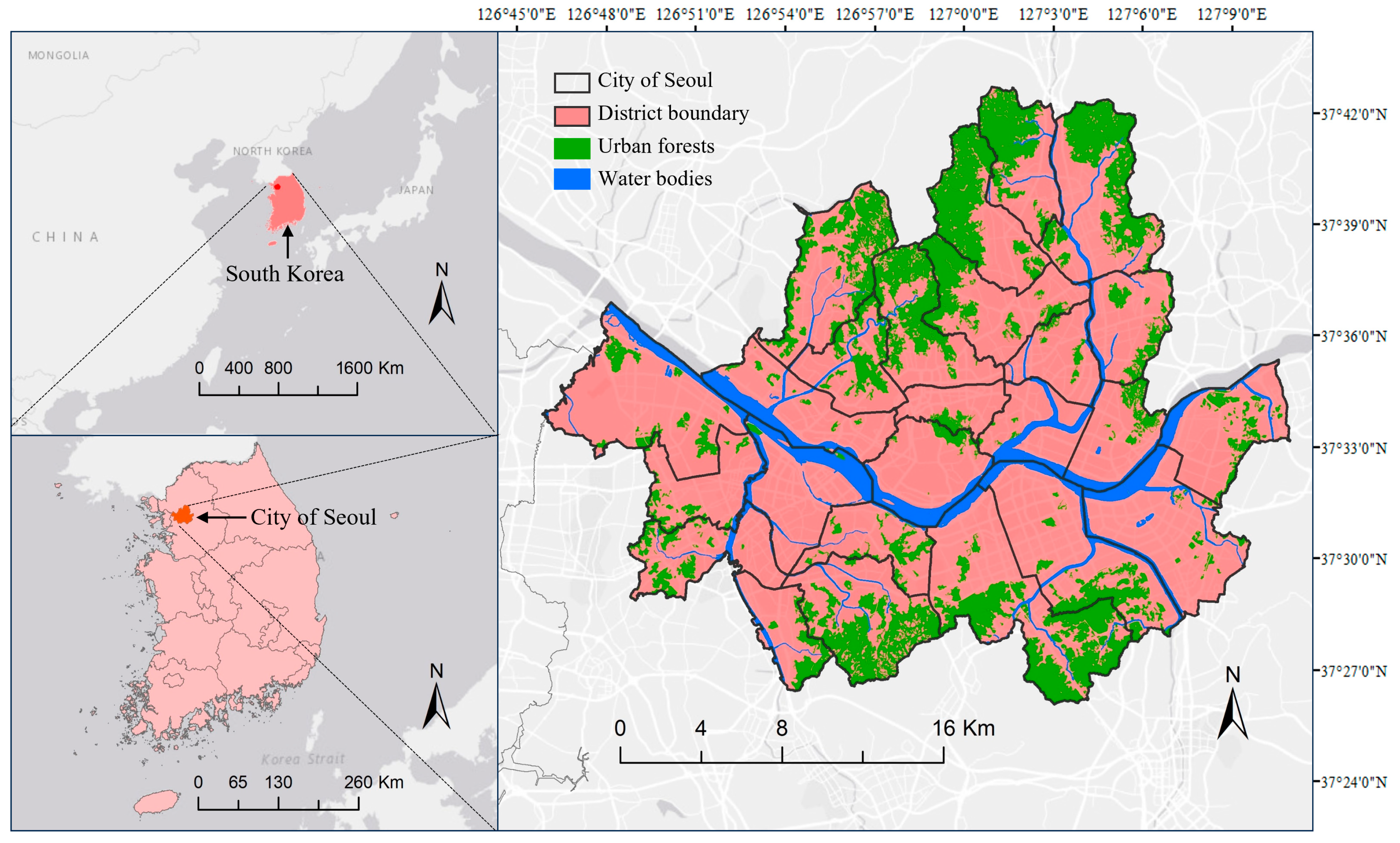
Figure 2.
Comparison of grid-based and street block-based units: (a) grid unit, (b) block unit.

Figure 3.
Seasonal distributions of land surface temperature (LST) in 2017, Seoul, South Korea: (a) spring, (b) summer, (c) autumn, and (d) winter.
Figure 3.
Seasonal distributions of land surface temperature (LST) in 2017, Seoul, South Korea: (a) spring, (b) summer, (c) autumn, and (d) winter.

Figure 4.
Partition of four quadrants as the intersection of summer and winter LSTs.

Figure 5.
Gravity index for urban forests (GIUF): (a) grid level, (b) block level.

Figure 6.
Gravity index for water bodies (GIWB): (a) grid level, (b) block level.

Figure 7.
Spatial distribution of the summer–winter LST quadrants in Seoul: (a) grid cell level; (b) street block level results.
Figure 7.
Spatial distribution of the summer–winter LST quadrants in Seoul: (a) grid cell level; (b) street block level results.


Table 1.
Date and time of Landsat 8 thermal infrared (TIR) image collection and temperature statistics.
Table 1.
Date and time of Landsat 8 thermal infrared (TIR) image collection and temperature statistics.
| Collection | Spring | Summer | Autumn | Winter | |
|---|---|---|---|---|---|
| Date | 2017.03.19 | 2017.08.26 | 2017.11.14 | 2017.01.14 | |
| Time | 11:10 a.m. | 11:10 a.m. | 11:10 a.m. | 11:11 a.m. | |
| LST (°C) | Mean | 19.8 | 34.5 | 12.8 | −2.7 |
| Max | 35.4 | 52.0 | 21.6 | 5.0 | |
| Min | 3.9 | 18.2 | −5.9 | −18.5 | |
| AT (°C) (Korea Meteorological Administration (KMA) weather history: https://www.weather.go.kr/w/obs-climate/land/past-obs/obs-by-day.do) (accessed on 16 June 2023) | Mean | 10.9 | 24.2 | 7.5 | −8.4 |
| Max | 18.9 | 29.2 | 11.4 | −5.4 | |
| Min | 3.2 | 19.0 | 2.9 | −10.4 | |
Table 2.
List of variables and descriptions.
| Category | Variables | Unit | Source | ||
|---|---|---|---|---|---|
| Dependent | Seasonal land surface temperature (LST) | °C | Landsat 8 TIR | ||
| Explanatory | Vegetation | Seasonal normalized difference in vegetation index (NDVI) | [0~1] | Landsat 8 OLI | |
| Land use | Land use type proportion | Residential | % | Korea Environmental Geographic Information Service (EGIS) 2017 | |
| Commercial | % | ||||
| Industrial | % | ||||
| Cultural and Recreational | % | ||||
| Transport | % | ||||
| Public | % | ||||
| Other uses | % | ||||
| Land use diversity | Entropy index | [0~1] | |||
| Reflectance | Albedo | % | Landsat 8 OLI | ||
| Building | 2-D | Building density | Count /10,000 m2 | Korea National Geographic Information Institute (NGII) 2017 | |
| Percent old buildings (+35 years) | % | ||||
| Average building coverage ratio (BCR) | % | ||||
| 3-D | Average floor area ratio (FAR) | % | |||
| Average total floor area | m2 | ||||
| Average building height | m | ||||
| Natural Area | Proximity to natural areas | Gravity index for urban forests | m2 | EGIS 2017 | |
| Gravity index for rivers and streams | m2 | ||||
Table 3.
Descriptive statistics for LST and the explanatory variables aggregated at the grid level (100 m 100 m) (N = 31,347).
Table 3.
Descriptive statistics for LST and the explanatory variables aggregated at the grid level (100 m 100 m) (N = 31,347).
| Category | Variable | Mean | Std. Dev. | Min. | Max. | |
|---|---|---|---|---|---|---|
| LST | LST (°C) | Spring | 20.69 | 1.62 | 11.00 | 31.20 |
| Summer | 37.38 | 2.31 | 25.25 | 49.86 | ||
| Autumn | 13.30 | 1.09 | −2.68 | 20.22 | ||
| Winter | −2.36 | 1.06 | −11.77 | 3.90 | ||
| Vegetation | NDVI (0~1) | Spring | 0.31 | 0.04 | 0.16 | 0.65 |
| Summer | 0.43 | 0.09 | 0.21 | 0.90 | ||
| Autumn | 0.28 | 0.03 | 0.15 | 0.48 | ||
| Winter | 0.17 | 0.02 | 0.11 | 0.43 | ||
| Land | Albedo (%) | Spring | 10.32 | 1.51 | 0.00 | 28.92 |
| Summer | 12.38 | 1.97 | 0.00 | 45.44 | ||
| Autumn | 6.61 | 1.32 | 0.00 | 33.60 | ||
| Winter | 5.16 | 1.26 | 0.00 | 27.88 | ||
| Land use type proportion (%) | Residential | 16.99 | 19.97 | 0.00 | 100.00 | |
| Commercial | 15.88 | 24.59 | 0.00 | 100.00 | ||
| Industrial | 0.44 | 4.88 | 0.00 | 100.00 | ||
| Cultural and Recreational | 0.83 | 5.95 | 0.00 | 99.87 | ||
| Transport | 44.16 | 37.50 | 0.00 | 100.00 | ||
| Public | 4.74 | 14.21 | 0.00 | 100.00 | ||
| Other uses | 17.00 | 29.38 | 0.00 | 100.00 | ||
| Land use Diversity (0~1) | Entropy Index | 0.27 | 0.17 | 0.00 | 0.71 | |
| Building | 2-D form | Building density (/10,000 m2) | 16.25 | 17.41 | 0.00 | 180.00 |
| % of old buildings (+35 years) | 18.22 | 24.35 | 0.00 | 100.00 | ||
| Average building coverage ratio (%) | 35.05 | 25.39 | 0.00 | 90.00 | ||
| 3-D form | Average floor area ratio (%) | 127.72 | 124.18 | 0.00 | 1420.19 | |
| Average total floor area (m2) | 3059.99 | 10,260.07 | 0.00 | 426,719.15 | ||
| Average building height (m) | 14.68 | 16.90 | 0.00 | 284.00 | ||
| Natural Area | Proximity to nature | Gravity index for urban Forests (m2) | 21.45 | 29.01 | 0.00 | 436.64 |
| Gravity index for rivers and streams (m2) | 9.15 | 16.29 | 0.00 | 160.01 | ||
Table 4.
Descriptive statistics for LST and the explanatory variables aggregated at the street block level (N = 4544).
Table 4.
Descriptive statistics for LST and the explanatory variables aggregated at the street block level (N = 4544).
| Category | Variable | Mean | Std. Dev. | Min. | Max. | |
|---|---|---|---|---|---|---|
| Block | Street block area (m2) | 65,451.6 | 184,125.9 | 3071.2 | 11,526,268.3 | |
| LST | LST (°C) | Spring | 20.45 | 1.17 | 15.32 | 25.93 |
| Summer | 37.75 | 1.70 | 31.27 | 45.21 | ||
| Autumn | 13.31 | 0.80 | 8.40 | 17.04 | ||
| Winter | −2.50 | 0.76 | −5.94 | 1.07 | ||
| Vegetation | NDVI (0~1) | Spring | 0.30 | 0.03 | 0.21 | 0.45 |
| Summer | 0.41 | 0.05 | 0.31 | 0.74 | ||
| Autumn | 0.27 | 0.02 | 0.21 | 0.37 | ||
| Winter | 0.17 | 0.01 | 0.13 | 0.25 | ||
| Land | Albedo (%) | Spring | 9.99 | 0.85 | 7.39 | 15.00 |
| Summer | 11.97 | 1.16 | 8.05 | 22.38 | ||
| Autumn | 6.33 | 0.71 | 3.53 | 12.28 | ||
| Winter | 4.89 | 0.70 | 2.83 | 12.53 | ||
| Land use type proportion (%) | Residential | 25.25 | 18.76 | 0.00 | 83.92 | |
| Commercial | 16.08 | 13.24 | 0.00 | 74.33 | ||
| Industrial | 0.21 | 1.85 | 0.00 | 49.00 | ||
| Cultural and Recreational | 1.07 | 2.35 | 0.00 | 31.83 | ||
| Transport | 40.79 | 12.89 | 0.19 | 91.91 | ||
| Public | 3.09 | 4.10 | 0.00 | 48.87 | ||
| Other uses | 13.50 | 16.31 | 0.00 | 99.81 | ||
| Land use Diversity (0~1) | Entropy Index | 0.60 | 0.11 | 0.01 | 0.91 | |
| Building | 2-D form | Building density (/10,000 m2) | 20.96 | 16.01 | 0.00 | 95.80 |
| % of old buildings (+35 years) | 21.43 | 19.21 | 0.00 | 100.00 | ||
| Average building coverage ratio (%) | 49.28 | 14.65 | 0.00 | 82.94 | ||
| 3-D form | Average floor area ratio (%) | 184.84 | 114.62 | 0.00 | 1409.81 | |
| Average total floor area (m2) | 3564.85 | 13,382.49 | 0.00 | 426,719.15 | ||
| Average building height (m) | 18.29 | 15.41 | 0.00 | 250.73 | ||
| Natural Area | Proximity to nature | Gravity index for urban forests (m2) | 19.13 | 26.21 | 0.00 | 267.06 |
| Gravity index for rivers and streams (m2) | 7.71 | 13.06 | 0.00 | 98.58 | ||
Table 5.
Comparison of variable means among quadrants: grid level versus block level.
| Variables (Unit) | Summer–Winter LST Quadrants | |||
|---|---|---|---|---|
| Quadrant 1 (Hot-Warm) | Quadrant 2 (Cool-Warm) | Quadrant 3 (Cool-Cold) | Quadrant 4 (Hot-Cold) | |
| Grid level (N = 31,347) | ||||
| Count | 10,635 (33.9%) | 5080 (16.2%) | 9023 (28.8%) | 6609 (21.1%) |
| Summer LST * (°C) | 39.28 ** | 35.26 ** | 35.50 ** | 38.50 ** |
| Winter LST * (°C) | −1.56 ** | −1.59 ** | −3.36 ** | −2.88 ** |
| Summer NDVI * (0~1) | 0.40 ** | 0.51 ** | 0.45 ** | 0.39 ** |
| Winter NDVI * (0~1) | 0.17 ** | 0.19 ** | 0.17 ** | 0.16 ** |
| Building density (/10,000 m2) * | 22.43 ** | 4.35 ** | 8.15 ** | 26.51 ** |
| Percent old buildings * | 24.37 ** | 9.88 ** | 11.60 ** | 23.76 ** |
| Average BCR * (%) | 42.33 ** | 16.66 ** | 25.87 ** | 50.02 ** |
| Average FAR * (%) | 135.97 ** | 70.78 ** | 118.79 ** | 170.41 ** |
| Average TFA * (m2) | 1405.4 ** | 2924.8 ** | 6044.6 ** | 1751.7 ** |
| Average BH * (m) | 11.47 ** | 10.11 ** | 21.22 ** | 14.41 ** |
| GIUF * (m2) | 15.39 ** | 22.58 ** | 31.05 ** | 17.24 ** |
| GIWB * (m2) | 8.77 ** | 15.33 ** | 8.03 ** | 6.55 ** |
| Block level (N = 4544) | ||||
| Count | 1665 (36.6%) | 685 (15.1%) | 1361 (30.0%) | 833 (18.3%) |
| Summer LST * (°C) | 39.15 ** | 36.55 ** | 36.12 ** | 38.60 ** |
| Winter LST * (°C) | −1.92 ** | −1.97 ** | −3.25 ** | −2.86 ** |
| Summer NDVI * (0~1) | 0.39 ** | 0.44 ** | 0.43 ** | 0.39 ** |
| Winter NDVI * (0~1) | 0.17 ** | 0.18 ** | 0.17 ** | 0.16 ** |
| Building density * (/10,0002) | 28.62 ** | 11.19 ** | 11.56 ** | 29.02 ** |
| Percent old buildings * | 27.66 ** | 15.51 ** | 14.32 ** | 25.48 ** |
| Average BCR * (%) | 53.73 ** | 43.79 ** | 43.32 ** | 54.66 ** |
| Average FAR * (%) | 171.19 | 181.77 | 204.02 ** | 183.29 |
| Average TFA * (m2) | 1198.3 ** | 4904.1 | 7215.0 ** | 1229.9 ** |
| Average BH * (m) | 13.43 ** | 19.69 ** | 25.89 ** | 14.46 ** |
| GIUF * (m2) | 13.49 ** | 21.72 ** | 27.55 ** | 14.52 ** |
| GIWB * (m2) | 8.27 ** | 12.05 ** | 6.19 ** | 5.47 ** |
* According to the one-way ANOVA test, the mean differences between quadrants are statistically significant (p < 0.01). ** The mean differences against at least two other groups are statistically significant (p < 0.05).
Table 6.
Statistics for spatial regression model selection at grid and block levels.
| Unit | Statistics | Spring LST | Summer LST | Autumn LST | Winter LST |
|---|---|---|---|---|---|
| Grid | Moran’s I (error) | 222.6 *** | 233.1 *** | 246.0 *** | 215.0 *** |
| Lagrange Multiplier (lag) | 43,918.0 *** | 40,443.8 *** | 51,506.0 *** | 41,759.4 *** | |
| Robust LM (lag) | 4092.0 *** | 2816.3 *** | 939.4 *** | 2136.2 *** | |
| Lagrange Multiplier (error) | 49,414.6 *** | 54,189.2 *** | 60,385.2 *** | 46,104.9 *** | |
| Robust LM (error) | 9588.6 *** | 16,561.7 *** | 9818.6 *** | 6481.7 *** | |
| Block | Moran’s I (error) | 49.1 *** | 53.6 *** | 55.1 *** | 47.2 *** |
| Lagrange Multiplier (lag) | 681.5 *** | 513.0 *** | 860.3 *** | 1738.3 *** | |
| Robust LM (lag) | 50.7 *** | 46.8 *** | 13.5 *** | 51.4 *** | |
| Lagrange Multiplier (error) | 2384.0 *** | 2837.1 *** | 3008.1 *** | 2203.5 *** | |
| Robust LM (error) | 1753.2 *** | 2370.9 *** | 2161.2 *** | 516.6 *** |
*** p-value < 0.01
Table 7.
General spatial model (GSM) estimation results at the grid level (N = 31,347).
| Variable | Spring LST | Summer LST | Autumn LST | Winter LST | |
|---|---|---|---|---|---|
| Constant | 1.7117 *** | 15.210 *** | 1.5375 *** | −3.453 *** | |
| NDVI | 3.8497 *** | −3.671 *** | 3.8345 *** | 8.489 *** | |
| Albedo | 0.1373 *** | 0.0643 *** | 0.1182 *** | 0.1761 *** | |
| Land use proportion | Residential | −0.0009 *** | 0.0051 *** | 0.0028 *** | 0.0024 *** |
| Commercial | 0.0029 *** | 0.0094 *** | 0.0047 *** | 0.0038 *** | |
| Industrial | 0.0090 *** | 0.0160 *** | 0.0088 *** | 0.0051 *** | |
| Cultural and Recreational | 0.0153 *** | 0.0244 *** | 0.0087 *** | 0.0076 *** | |
| Transport | 0.0056 *** | 0.0109 *** | 0.0073 *** | 0.0074 *** | |
| Public | 0.0030 *** | 0.0114 *** | 0.0040 *** | 0.0022 *** | |
| Land-use mix | Entropy Index | −0.2552 *** | −0.1454 *** | −0.1846 *** | −0.1842 *** |
| Building 2-D form | Count of buildings | 0.0094 *** | 0.0142 *** | 0.0073 *** | 0.0043 *** |
| % of old buildings (+35 years) | 0.0014 *** | 0.0025 *** | 0.0005 *** | 0.0003 *** | |
| Average building coverage ratio (BCR) | 0.0029 *** | 0.0053 *** | 0.0014 *** | 0.0008 *** | |
| Building 3-D form | Average floor area ratio | −0.0004 *** | −0.0006 *** | −0.0001 *** | 0.0000 |
| Average total floor area | −1.0 10-6 * | −1.0 10-6 ** | −2.0 10-6 *** | −2.0 10-6 *** | |
| Average building height | −0.0033 *** | −0.0045 *** | −0.0001 | 0.0001 | |
| Natural areas | Gravity index for urban forests | −0.0023 *** | −0.0188 *** | −0.0028 *** | −0.0036 *** |
| Gravity index for water bodies | −0.0010 ** | −0.0140 *** | 0.0015 *** | 0.0053 *** | |
| Rho (ρ) | 0.783 *** | 0.602 *** | 0.715 *** | 0.674 *** | |
| Lambda (λ) | 0.653 *** | 0.837 *** | 0.747 *** | 0.704 *** | |
| Adj. R2 | 0.901 | 0.928 | 0.867 | 0.843 | |
| Std. Err. | 0.51 | 0.62 | 0.39 | 0.42 | |
| AIC | 30,942.3 | 43,219.4 | 15,409.4 | 17,783.5 | |
***: p-value < 0.01, **: p-value < 0.05, *: p-value < 0.1.
Table 8.
General spatial model (GSM) estimation results at the block level (N = 4544).
| Variable | Spring LST | Summer LST | Autumn LST | Winter LST | |
|---|---|---|---|---|---|
| Constant | 6.5829 *** | 21.304 *** | 4.5804 *** | −6.5914 *** | |
| NDVI | 3.6073 *** | −4.371 *** | 7.8906 *** | 10.8662 *** | |
| Albedo | 0.4423 *** | 0.1319 *** | 0.2806 *** | 0.4600 *** | |
| Land use proportion | Residential | 0.0003 | 0.0163 *** | 0.0101 *** | 0.0050 *** |
| Commercial | 0.0125 *** | 0.0297 *** | 0.0160 *** | 0.0085 *** | |
| Industrial | 0.0444 *** | 0.0914 *** | 0.0432 *** | 0.0173 *** | |
| Cultural and Recreational | 0.0449 *** | 0.0595 *** | 0.0209 *** | 0.0158 *** | |
| Transport | 0.0028 ** | 0.0182 *** | 0.0113 *** | 0.0083 *** | |
| Public | 0.0047 * | 0.0406 *** | 0.0075 *** | −0.0081 *** | |
| Land-use mix | Entropy Index | −0.1979 *** | −0.0415 | −0.0919 *** | −0.0797 *** |
| Building 2-D form | Building density (100 m2) | 0.0165 *** | 0.0253 *** | 0.0098 *** | 0.0057 *** |
| % of old buildings (+35 years) | 0.0047 *** | 0.0073 *** | 0.0013 *** | 0.0006 | |
| Average building coverage ratio (BCR) | 0.0047 *** | 0.0053 *** | 0.0022 *** | 0.0016 ** | |
| Building 3-D form | Average floor area ratio | −0.0008 *** | −0.0011 *** | −0.0002 *** | −0.0001 |
| Average total floor area | 4.0 10−6 *** | 4.0 10−6 *** | 0.00 | −1.0 10−6 | |
| Average building height | −0.0087 *** | −0.0119 *** | −0.0027 *** | −0.0029 *** | |
| Natural areas | Gravity index for urban forests | −0.0007 * | −0.0098 *** | −0.0032 *** | −0.0036 *** |
| Gravity index for water bodies | 0.0018 * | −0.0046 *** | 0.0020 ** | 0.0071 *** | |
| Rho (ρ) | 0.388 *** | 0.384 *** | 0.282 | 0.227 *** | |
| Lambda (λ) | 0.463 *** | 0.508 *** | 0.607 | 0.560 *** | |
| Adj. R2 | 0.730 | 0.813 | 0.674 | 0.636 | |
| Std. Err. | 0.61 | 0.73 | 0.46 | 0.46 | |
| AIC | 5616.4 | 7390.3 | 3132.8 | 3113.9 | |
*** p-value < 0.01, ** p-value < 0.05, * p-value < 0.1.
Disclaimer/Publisher’s Note: The statements, opinions and data contained in all publications are solely those of the individual author(s) and contributor(s) and not of MDPI and/or the editor(s). MDPI and/or the editor(s) disclaim responsibility for any injury to people or property resulting from any ideas, methods, instructions or products referred to in the content. |
© 2023 by the authors. Licensee MDPI, Basel, Switzerland. This article is an open access article distributed under the terms and conditions of the Creative Commons Attribution (CC BY) license (https://creativecommons.org/licenses/by/4.0/).
Share and Cite
MDPI and ACS Style
Jeon, G.; Park, Y.; Guldmann, J.-M. Impacts of Urban Morphology on Seasonal Land Surface Temperatures: Comparing Grid- and Block-Based Approaches. ISPRS Int. J. Geo-Inf. 2023, 12, 482. https://doi.org/10.3390/ijgi12120482
AMA Style
Jeon G, Park Y, Guldmann J-M. Impacts of Urban Morphology on Seasonal Land Surface Temperatures: Comparing Grid- and Block-Based Approaches. ISPRS International Journal of Geo-Information. 2023; 12(12):482. https://doi.org/10.3390/ijgi12120482
Chicago/Turabian StyleJeon, Gyuwon, Yujin Park, and Jean-Michel Guldmann. 2023. "Impacts of Urban Morphology on Seasonal Land Surface Temperatures: Comparing Grid- and Block-Based Approaches" ISPRS International Journal of Geo-Information 12, no. 12: 482. https://doi.org/10.3390/ijgi12120482
Note that from the first issue of 2016, this journal uses article numbers instead of page numbers. See further details here.