Mapping Gross Domestic Product Distribution at 1 km Resolution across Thailand Using the Random Forest Area-to-Area Regression Kriging Model

Abstract

Accurate spatial distribution of gridded gross domestic product (GDP) data is crucial for revealing regional disparities within administrative units, thus facilitating a deeper understanding of regional economic dynamics, industrial distribution, and urbanization trends. The existing GDP spatial models often rely on prediction residuals for model evaluation or utilize residual distribution to improve the final accuracy, frequently overlooking the modifiable areal unit problem within residual distribution. This paper introduces a hybrid downscaling model that combines random forest and area-to-area kriging to map gridded GDP. Employing Thailand as a case study, GDP distribution maps were generated at a 1 km spatial resolution for the year 2015 and compared with five alternative downscaling methods and an existing GDP product. The results demonstrate that the proposed approach yields higher accuracy and greater precision in detailing GDP distribution, as evidenced by the smallest mean absolute error and root mean squared error values, which stand at USD 256.458 and 699.348 ten million, respectively. Among the four different sets of auxiliary variables considered, one consistently exhibited a higher prediction accuracy. This particular set of auxiliary variables integrated classification-based variables, illustrating the advantages of incorporating such integrated variables into modeling while accounting for classification characteristics.

1. Introduction

Socioeconomic parameters play essential roles in government management, enterprise decision-making, and scientific research, often acquired through traditional statistical surveys. However, these data often fail to reveal the inner spatial differences of irregular administrative units, posing a challenge for understanding the complex interactions between human beings and the environment [1]. To overcome this limitation and obtain high-spatial-resolution socioeconomic data, spatialization studies have been developed to allocate such data from statistical units to regular grids [2,3,4]. Among the various socioeconomic parameters, gross domestic product (GDP) holds particular significance as the broadest measure of economic development and resource allocation on national and local scales [5]. While GDP data from statistical units provide valuable insights, gridded GDP data with fine regular grid cells offer a more detailed spatial distribution of GDP counts within each statistical unit (i.e., administrative unit). Moreover, these gridded GDP data can be effectively integrated with other raster geoscience variables, such as remotely sensed data from Earth observation satellites, enabling spatial analyses in both raster and vector formats [6]. Consequently, the importance of downscaling statistical GDP (i.e., GDP spatialization or GDP prediction in space) has been increasingly recognized, leading to the widespread adoption of gridded GDP data in various applications.

The theoretical foundation of GDP spatialization lies in the strong relationship between anthropogenic lighting signals at night (nighttime light, NTL) and economic activity, which was first reported in [7]. To explore this relationship, the earliest satellite-derived NTL data came from the US Air Force Defense Meteorological Satellite Program-Operational Linescan System (DMSP-OLS), including daily, monthly, and annual data, developed by the NOAA National Geophysical Data Center (NGDC) and ranging from 1992 to 2013 [8,9]. Notably, Doll et al. [10] produced the first global gridded GDP map with a 1° resolution using DMSP-OLS NTL data. Subsequently, newer NTL data have been acquired from the Suomi National Polar-Orbiting Partnership satellite (NPP) since 2012 [11]. Compared to DMSP-OLS NTL data, NPP-VIIRS NTL data from the Visible Infrared Imaging Radiometer Suite (VIIRS) offer superior in-flight calibration, higher spatial resolution, lower detection limit, wider dynamic range, and finer radiometric quantization [12]. As a result, NPP-VIIRS NTL data can generate gridded GDP maps with even finer resolution [13]. Recently, the latest version of synthetic annual NPP-VIIRS NTL data, developed in [14], has gained wide acceptance and has been used to examine economic activity in various studies [15,16,17,18,19,20,21,22]. Despite its potential, few studies have explored gridded GDP prediction using this version of the NPP-VIIRS NTL data.

Despite the successful application of GDP spatialization in various regions, including 11 European Union countries and the United States [23], different administrative units in China [6,24,25,26,27], the continental United States (CONUS) [28], and the entire world [29,30,31], few studies have considered the impacts of different sectors in GDP spatialization [15,19]. Studies have shown that NTL data alone are insufficient to explain GDP from agriculture and forestry [32].To overcome this limitation, a more effective method is to combine NTL with land use/land cover (LULC) data and other auxiliary data, such as vegetation index, to predict and spatialize GDP in different sectors [6,24,25,29]. Recent studies have utilized vegetation index together with NTL and LULC data to spatialize primary industry GDP in Turkey and China [33,34]. Moreover, Wang et al. [31] employed gridded population data, statistical agricultural output data, and market price data of different crops to spatialize agricultural GDP in Uganda. However, there remains a lack of studies exploring the estimation of non-agricultural and agricultural GDP separately, particularly using the new version of the NPP-VIIRS data.

The methods for GDP spatialization have undergone evolution over the past three decades. Initially, researchers heavily relied on linear regression models, exponential linear models, and multiple linear fitting for GDP prediction [3,10,25,26,29,30,31,35]. It has been increasingly recognized that using NTL data alone is insufficient for achieving accurate GDP prediction. As a result, researchers have turned to employing multiple linear fitting alongside auxiliary data, such as land use/land cover (LULC) data, environmental data, and population data, to enhance the accuracy of GDP spatialization [6,31]. In recent years, machine learning techniques, such as convolutional neural networks and random forests, have emerged in tandem with geospatial big data, offering new opportunities to improve the spatial prediction of GDP [2,15,28,34]. Conventionally, the residuals predicted by the aforementioned models have served as a yardstick for assessing the performance of GDP prediction models. Additionally, some studies have employed residual allocation methods to address potential biases in spatial scales. These methods allocate the residuals at the target spatial scale, ensuring unbiased results at the original spatial scale [23,26,36]. Researchers have successfully applied these residual allocation methods in studies utilizing multiple linear fitting and random forests to improve the accuracy of GDP spatialization [27,33]. However, it is worth noting that some studies have simply corrected residuals in space by multiplying the ratio of the actual GDP to forecast GDP, without accounting for potential modifiable areal unit problems.

Hence, this paper introduces a sub-sector downscaling strategy based on a hybrid approach that combines random forest algorithm (RF) and area-to-area kriging (ATAK) interpolation to map the GDP across Thailand at a 1 km spatial resolution. Subsequently, we conducted an assessment of the potential of various combinations of ancillary variables in enhancing GDP prediction by incorporating the latest version of the NPP-VIIRS data, points of interest, vegetation index, and other relevant data. To achieve this, we established distinct random forest area-to-area regression kriging (RFATARK) models for both agricultural and non-agricultural GDP, incorporating four distinct groups of ancillary variables. A comparative analysis of the downscaled GDP results from five alternative methodologies underscored the notable advantages of the RFATARK-based downscaling approach. This advantage was further validated through a comparison with an alternate gridded GDP product. The structure of the paper is as follows: Section 2 provides insights into the study area, data sources, and the specific methodology deployed for GDP spatialization. Subsequently, Section 3 presents the outcomes of our analytical endeavors, followed by a comprehensive discussion in Section 4. The conclusive Section 5 encapsulates the inferences derived from our research.

2. Materials and Methods

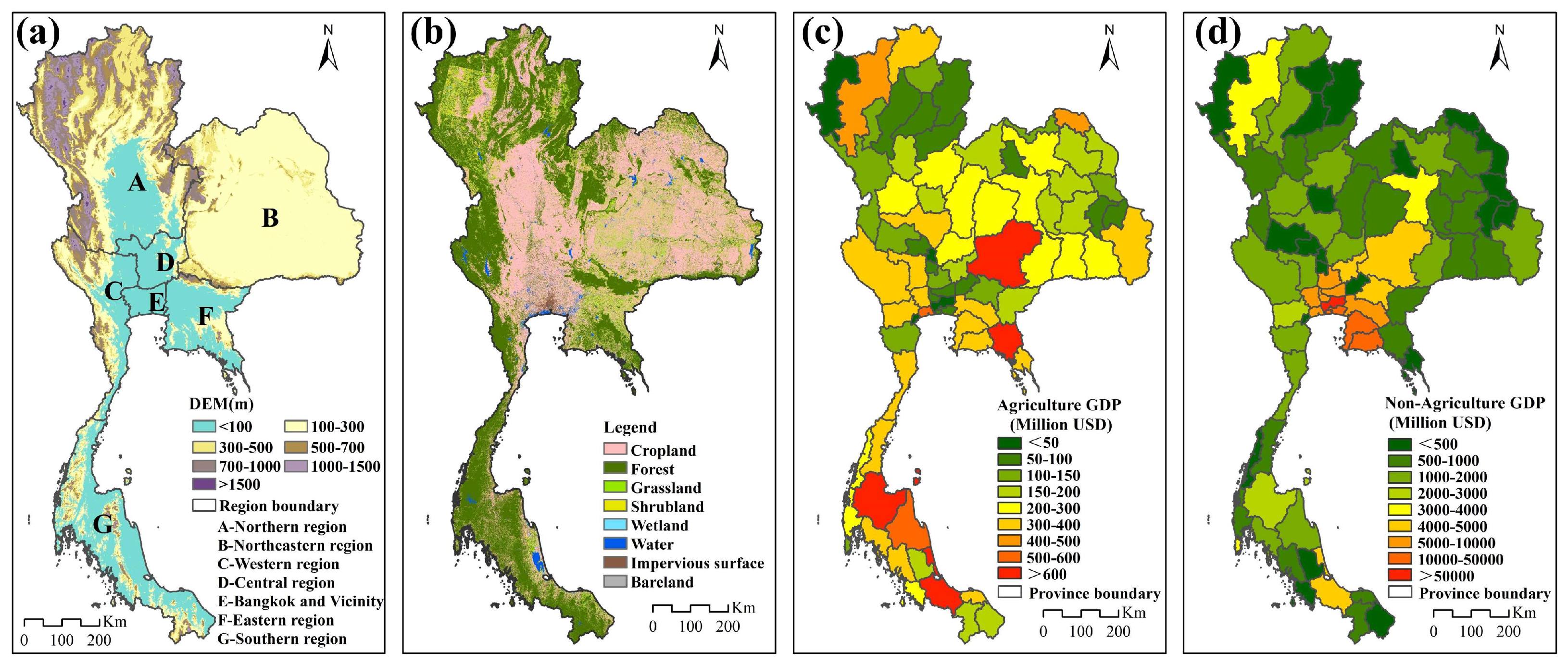
2.1. Study Area

The study is centered within the Kingdom of Thailand, located in tropical Southeast Asia on the Indochina Peninsula, encompassing an approximate land area of 513,000 km² (Figure 1). Bordered by Myanmar to the north and west, Thailand’s northeastern boundary is delineated by the Mekong River, adjacent to Laos. To the east lies Cambodia, while the southern region extends as a narrow peninsula between the Andaman Sea and the Gulf of Thailand, adjoining northern Malaysia. As a significant member of the Association of Southeast Asian Nations (ASEAN), Thailand serves as a primary conduit for China’s access to the Indian Ocean via the Indochina Peninsula, signifying its strategic role within China’s “One Belt and One Road” (OBOR) initiative [37].

The geographical features of Thailand are varied and contribute significantly to its regional diversity. Northern Thailand is characterized by extensive forest cover, whereas the northeastern plateau, known as the Khurat Plateau, faces challenges in agriculture due to its dry summers and rainy wet seasons. The southern peninsula extends from the western mountain range, featuring hills in the west and coastal plains in the east. The central plain, nourished by the Chao Phraya River, historically serves as the nation’s rice belt for agricultural production. The administrative divisions in Thailand encompass seven regions: the northern region, northeastern region, western region, central region, Bangkok and vicinity, eastern region, and southern region. The nation is subdivided into 77 provinces, with the capital city, Bangkok, holding a unique status as both the political center and the sole municipality under direct central government jurisdiction.

Thailand’s climate is decidedly tropical and exhibits three distinct seasons: summer (mid-February to mid-May), the rainy season (mid-May to mid-October), and winter (mid-October to mid-February). The country experiences temperatures ranging from 18 °C to 36 °C, accompanied by an average annual rainfall of approximately 1700 mm.

The country’s geographical and climatic characteristics significantly influence its agricultural landscape, which spans 265,200 km², including 49,600 km² of irrigated land. Thailand’s stature as the world’s largest exporter of rice and natural rubber underscores its agricultural prominence [38]. The nation’s maritime significance is underscored by its position as the third-largest fishing country in Asia, attributed to its abundant marine fisheries in the Gulf of Thailand and Andaman Sea. In 2015, Thailand’s Gross Domestic Product (GDP) reached USD 401.3 million, with industry and services contributing 39.2%, agriculture 8.4%, trade 13.4%, logistics technology and communication 9.8%, construction and mining 4.3%, and other service sectors, encompassing finance, education, and hospitality, comprising 24.9% [39].

2.2. Materials

The dataset employed in this study encompasses a synthesis of remote sensing data, geographic information data, and socioeconomic statistical data (as presented in

Table 1. Comprehensive datasets utilized in the present study.

Type	Dataset	Description	Source
①	NTL	Annual composited NPP/VIIRS nighttime light data Spatial resolution: 15 arc-seconds	Earth Observation Group at Payne Institute for Public Policy, Colorado School of Mines
	Vegetation index	Annual synthetic NDVI, EVI, and MODIS near-infrared vegetation reflectance index Spatial resolution: 250 m	Maximum value composite based on MODIS product (MOD13A3) or MODIS-based data calculated by MODIS Surface reflectance product (MOD43)
	Land surface temperature (LST)	Annual synthetic LST Spatial resolution: 1000 m	Maximum value composite based on MODIS product (MYD11A1)
	LULC	Finer Resolution Observation and Monitoring—Global Land Cover Spatial resolution: 30 m	FROM-GLC at Tsinghua University
②	Terrain data: digital elevation model (DEM)	ASTER/GDEM Spatial resolution: 30 m	Earth Remote Sensing Data Analysis Center of Japan
	Boundary information	Provincial boundaries	Database of Global Administrative Areas
	Road, water, and point of interest (POI)	Road network, water bodies, and water roads, and 13 types of POIs of Thailand	Open Street Map (OSM) from Geofabrik GmbH
③	GDP statistical and census data	Total GDP and population of the 77 provinces in Thailand	Office of the Thailand Economic and Social Development Council
	Gridded GDP data	GDP of each grid cell Spatial resolution: 30 arc-seconds	Kummu et al. (2018)
	Population (Worldpop)	Grided population count datasets Spatial resolution: 100 m	University of Southampton

Note: ① is remote sensing data, ② is geographic information data, ③ is socioeconomic statistical data.

).

The remote sensing data assimilated within this study encompass NTL, vegetation index (VI), LST, and LULC. The NTL data utilized in this investigation were derived from the NPP/VIIRS day/night band (DNB) dataset, acquired from the Earth Observation Group (EOG) at the Payne Institute for Public Policy, Colorado School of Mines (https://eogdata.mines.edu/products/vnl/, accessed on 6 December 2022). Specifically, the annual imagery for the year 2015 was employed, with a spatial resolution of 15 arc-seconds (~500 m at the equatorial regions) presented as geographic grids. The NTL values are expressed in digital number (DN) format. The ‘vcm-orm-ntl’ annual synthetic product, the first version, was utilized in this study, which involved filtering out transient lights, stray light, background values, and anomalous data, resulting in cloudless average radiation values [14]. The vegetation index data, encompassing normalized difference vegetation index (NDVI), enhanced vegetation index (EVI), and near-infrared vegetation index (NIRv), were calculated utilizing MODIS reflectance data, specifically the MCD43A4.006 BRDF-Adjusted Reflectance 16-Day L3 Global 500 m product. These data were hosted on Google Earth Engine and subjected to quality control using the quality assurance layer [40]. Calculation of the NIRv values followed the approach outlined in [41], while NDVI and EVI values were computed according to the methodology presented in [42]. LST data were drawn from MODIS LST data of the Aqua satellite, employing the MYD11A1.006 Land Surface Temperature/Emissivity Daily L3 Global 1 km dataset, available on Google Earth Engine [43]. The selection of the Aqua satellite data was influenced by its local overpass time of 13:30, closely aligning with the occurrence of daily maximum temperatures. The LULC data were procured from the FROM-GLC dataset developed in [44], with a spatial resolution of 30 m, accessible at http://data.ess.tsinghua.edu.cn/ (accessed on 24 March 2023).

The geographic information data encompass digital elevation model (DEM), boundary information, road networks, water bodies, and points of interest (POIs). The DEM data, sourced from Advanced Space Borne Thermal Emission and Reflection Radiometer (ASTER)/Global Digital Elevation Model (GDEM), had a spatial resolution of 30 m and were provided by the Earth Remote Sensing Data Analysis Center of Japan [45]. Boundary information data were procured from the GADM data repository (https://gadm.org/data.html, accessed on 14 June 2022), specifically version 3.6. The road, water, and POI data were sourced from the OpenStreetMap (OSM) project, renowned for generating and distributing free global geographic data (download URL: http://download.geofabrik.de/asia/thailand.html, accessed on 20 December 2022).

The socioeconomic statistical data at the provincial level in Thailand, encompassing GDP statistical data and census data, were acquired from the Thailand Economic and Social Development Council (https://www.nesdc.go.th/nesdb_en/, accessed on 13 January 2022). The gridded GDP (G_GDP) dataset by Kummu et al. [46] is accessible at https://datadryad.org/stash/dataset/doi:10.5061/dryad.dk1j0 (accessed on 25 December 2022). Gridded population data from Worldpop, created by the University of Southampton, is accessible at https://www.worldpop.org/ (accessed on 7 December 2022) [47].

2.3. Data Processing

The collected data underwent a series of preprocessing steps, including the calculation of relevant indicators, all of which served as auxiliary variables for GDP spatialization. The resulting auxiliary variable data were subsequently resampled to achieve a final spatial resolution of 1 km.

2.3.1. NTL Data Processing

Bangkok, as Thailand’s most developed city, served as a critical reference point in the analysis of nighttime light (NTL) data. The fundamental assumption is that pixel values in other regions should not theoretically exceed the values observed in Bangkok. Therefore, the highest Digital Number (DN) value recorded in Bangkok was employed as a threshold to identify outliers in other areas. Additionally, to ensure compatibility with other datasets, the spatial resolution of the NPP/VIIRS NTL data was resampled from 15 arc-seconds to 500 m using the nearest neighbor method. Subsequently, these resampled NPP/VIIRS NTL data were employed to compute four essential nighttime light indices, Averaged Nighttime Light (NLAve), Nighttime Light Intensity (NLVI), Nighttime Light Lit Area Proportion (NLVS), and Compounded Nighttime Light Index (VCNLI), following the approach outlined by Zhao et al. [13].

NLAve represents the average DN value of the NPP/VIIRS NTL data within a given statistical unit. It is computed using the formula:

$$\mathrm{NLAve}=\frac{\sum {\mathit{DN}}_{\mathit{i}}\times {\mathit{n}}_{\mathit{i}}}{\mathit{S}}$$

(1)

where DN_i and n_i denote the pixel value of the light level and the corresponding pixel count within a statistical unit, respectively. S represents the total area of the statistical unit in square kilometers.

NLVI is defined as the ratio of NLAve to the maximum nighttime light value within a statistical unit. The calculation is as follows:

$$\mathrm{NLVI}=\mathrm{NLAve}/\left({\mathit{DN}}_{\max }\times {\mathit{N}}_{\mathit{L}}/\mathit{S}\right)$$

(2)

where DN_max is the maximum DN value in the NPP/VIIRS NTL data, and N_L represents the total number of lit pixels within a statistical unit.

NLVS is determined by the ratio of the lit pixel area (SL) to the total area of the statistical unit (S), as indicated below:

$$\mathrm{NLVS}={\mathit{S}}_{\mathit{L}}/\mathit{S}$$

(3)

VCNLI is calculated as the product of NLVI and NLVS, providing a comprehensive measure of nighttime light characteristics within a statistical unit:

$$\mathrm{VCNLI}=\mathrm{NLVI}\times \mathrm{NLVS}$$

(4)

2.3.2. OSM Data Processing

The OSM dataset encompasses road data, water data, and POI data, as detailed in

Table 2. Introduction and weighting of OSM auxiliary variables for both road and water data.

Class	Content	Group	Weight (Class)	Weight (Group)
Major roads	Motorways, primary roads, secondary roads, tertiary roads.	Road1	0.148	0.263
Rail	Railways.	Road1	0.131
Highway links	Roads that connect from one road to another.	Road2	0.133	0.247
Subway	Subways.	Road2	0.092
Minor roads	Smaller local roads, roads in residential areas, streets.	Road3	0.147	0.251
Paths	Paths unsuitable for cars.	Road3	0.113
Small roads	Paths for cycling, footpaths, gravel roads, etc.	Road4	0.135	0.239
Unknown	Unknown type of road or path.	Road4	0.101
River	Large rivers.	Water1	0.137	0.231
Reservoir	Artificial lakes.	Water1	0.111
Stream	Smaller rivers or streams.	Water2	0.124	0.294
Canal	Canals.	Water2	0.125
Wetland	Swamp, bog, or marsh land.	Water3	0.153	0.204
Water	Unspecified bodies of water.	Water3	0.104
Drain	Small drainage ditches or similar structures.	Water4	0.124	0.271
Dock	Docks.	Water4	0.122

and

Table 3. Introduction and weighting of OSM auxiliary variables for POI data.

Class	Content	Weight
Accommodation	Hotels, motels, guesthouses, hostel, etc.	0.092
Catering	Restaurants, bars, cafes, etc.	0.102
Health	Pharmacies, hospitals, veterinaries, etc.	0.084
Leisure	Theaters, playgrounds, parks, cinemas, stadiums, etc.	0.093
Fuel and parking	Gas stations, service areas, car parks, etc.	0.056
Money	Banks, ATMs, etc.	0.104
Public	Police posts, fire stations, post offices, libraries, schools, etc.	0.064
Village and hamlet	Villages and hamlets.	0.031
Tourism	Tourist attractions, museums, monuments, zoos, ruins, etc.	0.077
Pofw	Buddhist temples, churches, synagogues, mosques, Muslim places, etc.	0.050
Miscpoi	Toilets, fountains, fire hydrants, towers, etc.	0.066
Shopping	Supermarkets, bakeries, malls, travel agencies, vending machines, etc.	0.094
Transport	Railway stations, bus stops, subway stations, airports, etc.	0.087

. In this subsection, we provide a comprehensive description of the processing steps undertaken for each type of OSM data.

For both road and water data, we calculated the auxiliary variables by determining the distance from the center point of each 1 km × 1 km pixel to the nearest road or water feature within each respective class. This information assumes a critical role in subsequent analyses.

For the POI data, we generated ten gridded (1 km × 1 km) auxiliary variables, each corresponding to ten types of POI point data. This was achieved through the application of kernel density estimation (KDE), following the methodology detailed by Wang et al. [48]. An integral aspect of KDE is the bandwidth parameter, which we meticulously determined. Our process encompassed the exploration of a bandwidth range spanning from 500 m to 25 km. Within this range, we adopted a step length of 100 m for distances ranging from 500 to 10,000 m, and a 1 km step length for distances between 10 and 25 km. Consequently, this procedure yielded 110 distinct bandwidth values, consequently generating 1100 gridded POI density layers (comprising 10 types of POIs and 110 bandwidths). These layers were aggregated to the provincial scale through an average aggregation method. Subsequently, we constructed random forest (RF) models at the provincial scale, with each bandwidth corresponding to a unique RF model. The ten gridded POI density layers generated for each bandwidth served as independent variables, while provincial Gross Domestic Product (GDP) was employed as the dependent variable. Among the 110 RF models, we discerned the optimal bandwidth by identifying the bandwidth that minimized the out-of-bag error value (i.e., normalized mean square error (MSE)), a determination illustrated in Figure 2. Notably, the optimal bandwidth was determined to be 8100.

Concerning the treatment of OSM auxiliary variables, we administered four distinct approaches based on a combination of two processing methods. The two methods considered were the classification of water and road auxiliary variables and the merging of OSM auxiliary variables. These four treatments are as follows: (1) Unmerged and Single (UMS): water and road auxiliary variables remained unclassified, and POI auxiliary variables were left unmerged; (2) Unmerged and Classified (UMC): while water and road auxiliary variables were classified, POI auxiliary variables were not subjected to merging; (3) Merged and Single (MS): water, road and POI auxiliary variables were merged without any classifying; and (4) Merged and Classified (MC): involved the merged water, road and POI auxiliary variables, in which the water and road auxiliary variables were classified.

The merging of OSM auxiliary variables was executed through a weighted approach [49], as described by Equation (5):

$${\mathit{OSM}}_{\mathrm{sum}}={\sum }_{\mathit{j}=1}^{\mathit{m}}{\mathit{w}}_{\mathit{j}}{\mathit{b}}_{\mathit{ij}}$$

(5)

where ${\mathrm{OSM}}_{\mathrm{sum}}$ represents the merged OSM auxiliary variable for different types; $b_{ij}$ is the value of the j-th OSM auxiliary variable for the i-th pixel after normalization; $m$ denotes the count of one type of OSM auxiliary variables; and $w_j$ indicates the weight value of the j-th OSM auxiliary variable. These weight values of each class (or group) of OSM auxiliary variable are calculated through the entropy method, governed by Equations (6)–(8) [48]:

$${\mathit{b}}_{\mathit{ij}}=\frac{{\mathit{a}}_{\mathit{ij}}-\min \{{\mathit{a}}_{1\mathit{j}},\dots ,{\mathit{a}}_{\mathit{nj}}\}}{\max \left\{{\mathit{a}}_{1\mathit{j}},\dots ,{\mathit{a}}_{\mathit{nj}}\right\}-\min \{{\mathit{a}}_{1\mathit{j}},\dots ,{\mathit{a}}_{\mathit{nj}}\}}$$

(6)

$${\mathit{e}}_{\mathit{j}}=-\frac{1}{\ln \left(\mathit{n}\right)}\times {\sum }_{\mathrm{i}=1}^{\mathit{n}}\left(\left(\frac{{\mathit{b}}_{\mathit{ij}}}{{\sum }_{\mathit{i}=1}^{\mathit{n}}{\mathit{b}}_{\mathit{ij}}}\right)\times \ln \left(\frac{{\mathit{b}}_{\mathit{ij}}}{{\sum }_{\mathit{i}=1}^{\mathit{n}}{\mathit{b}}_{\mathit{ij}}}\right)\right)$$

(7)

$${\mathit{w}}_{\mathit{j}}=\frac{1-{\mathit{e}}_{\mathit{j}}}{{\sum }_{\mathit{j}=1}^{\mathit{m}}(1-{\mathit{e}}_{\mathit{j}})}$$

(8)

In these equations, ${\mathit{a}}_{\mathit{ij}}$ corresponds to the value of the j-th OSM auxiliary variable for the i-th pixel, n is the count of pixels in the auxiliary variable raster layer, and ${\mathit{e}}_{\mathit{j}}$ represents the entropy value of the j-th OSM auxiliary variable. The weight associated with each class of OSM auxiliary variables is presented in Table 2 and Table 3.

2.3.3. Other Processing

Beyond the above two data sources, five additional types of data play a crucial role in the GDP spatialization process. These encompass terrain data, land use and land cover (LULC) data, vegetation index data, land surface temperature (LST) data, and population data.

The cornerstone of terrain data lies in the Digital Elevation Model (DEM) data, characterized by a spatial resolution of 30 m. This initial dataset underwent a transformation process, resulting in the derivation of three fundamental parameters: elevation, slope, and slope direction. Subsequently, the elevation values at broader scales, specifically operating at a 1 km scale or the provincial scale, were computed through the aggregation of 30 m elevation values within individual statistical units. Furthermore, the determination of slope and slope direction at these elevated scales was achieved through an assessment of the proportion of slopes with inclinations less than 5 degrees and an examination of the distribution of slope directions, encompassing sunny slopes, semi-sunny slopes, semi-shady slopes, and shady slopes, within each statistical unit.

The LULC dataset employed for this study in Thailand comprises eight distinct land cover categories, conforming to the FROM-GLC classification system. These categories encompass crop, forest, grass, shrub, wetland (denoted as wet), water bodies, bare land (denoted as bare), and impervious surfaces. The analysis entailed the quantification of the relative abundance of these land cover classes within each statistical unit, operating at either a 1 km scale or the provincial level.

To discriminate human settlements from other land cover types and to ameliorate the impact of cloud interference, an annual synthetic vegetation index was generated through the application of the maximum value composite method to multitemporal vegetation index imagery. Subsequently, the vegetation index data underwent spatial aggregation, resulting in a resolution of 1 km through a process of averaging. This refined dataset was then amenable to the computation of vegetation index values per unit area, whether at the provincial level or within individual grid cells. Notably, it is imperative to emphasize that the LST data follow an analogous preprocessing procedure to that of the vegetation index data.

The gridded population data, sourced from the Worldpop database, underwent a meticulous calibration process, which harmonized it with census data to ensure data integrity and fidelity. Following this calibration, the population data were aggregated to a resolution of 1 km or the provincial scale.

2.4. Downscaling Methodology

The dataset employed in this study encompassed a synthesis of remote sensing data, geographic information data, and socioeconomic statistical data (as presented in Table 1).

2.4.1. Downscaling Model

A machine learning-based geostatistical downscaling method was introduced in this study, referred to as the RFATARK model (random forest area-to-area regression kriging). The RFATARK model combines two distinct techniques, namely the random forest (RF) algorithm, which is employed within the trend module, and the area-to-area kriging (ATAK) interpolation method, utilized within the residual module. The RF algorithm, initially proposed by Breiman [50] and further refined by Culter and Stevens [51], is a machine learning technique utilized for diverse tasks, including classification, regression, and other decision tree-based applications. Compared to traditional regression algorithms, the RF algorithm offers several advantages, such as a high predictive accuracy, the absence of prior probability distribution assumptions, and the capacity to assess variable importance [52]. The RF model involves two key parameters, which represents the number of variables used to make decisions at the nodes of decision trees (denoted as mtree), and indicates the number of decision trees generated (denoted as ntree). During the modeling process, mtry and ntree were optimized to determine the most suitable parameter settings based on error variations across different parameter combinations. On the other hand, ATAK, a variant of areal interpolation, changes the supports before and after the interpolation. Its purpose is to redistribute areal residuals to their target area-level positions [53]. This approach achieves the prediction of areal values through a linear combination of areal data. For each specific pixel, the residual is calculated as a weighted linear combination of residuals from neighboring areas, satisfying an unbiased weight constraint.

Let GDP(S_i) and X_k(S_i) represent the target and k ancillary random variables at coarse pixel S_i. The RF regression model capturing the relationship between GDP(S_i) and X_k(S_i) can be symbolized as f(·). Under the assumption of scale-invariance in the statistical relationships among these variables, the trend component of fine spatial resolution is estimated through the utilization of the coarse regression function. Subsequently, the residual component of the fine spatial resolution is determined through ATAK, which interpolates the coarse residuals by considering m neighboring coarse pixels, denoted as e(S_i). The predicted GDP at a 1 km resolution, represented as GDP(s), at the fine resolution using the RFATARK model, can be expressed as follows:

$$\mathrm{GDP}\left(\mathit{s}\right)=\mathit{f}\left({\mathit{x}}_{\mathit{k}}\left(\mathit{s}\right)\right)+{\sum }_{\mathit{i}=1}^{\mathit{m}}{\lambda }_{\mathit{i}}·\mathit{e}\left({\mathit{S}}_{\mathit{i}}\right)=\mathit{f}\left({\mathit{x}}_{\mathit{k}}\left(\mathit{s}\right)\right)+{\sum }_{\mathit{i}=1}^{\mathit{m}}{\lambda }_{\mathit{i}}·[\mathrm{GDP}\left({\mathit{S}}_{\mathit{i}}\right)-\mathit{f}\left({\mathit{x}}_{\mathit{k}}\left({\mathit{S}}_{\mathit{i}}\right)\right)]$$

(9)

where ${\lambda }_i$ represents the weight assigned to m neighboring coarse pixels in ATAK, satisfying the constraint ${\sum }_{i=1}^m{\lambda }_i\left(S_i\right)=1$. For a detailed calculation process, refer to [54].

In this study, the RFATARK model was applied separately to non-agricultural and agricultural statistical GDP, resulting in the mapping of non-agricultural and agricultural GDP at a 1 km resolution. Given the distinct characteristics of agricultural and non-agricultural GDP, land cover information was used to mask the GDP prediction results based on the following rules:

$${\mathrm{GDP}}_{\mathit{j}}^{\mathit{agri}}=0, \mathrm{if} \left\{\begin{array}{c}{\mathrm{L}}_{\mathrm{forest}}\ge 0.9\cap {\mathrm{L}}_{\mathrm{imp}}<0.1\\ {\mathrm{L}}_{\mathrm{crop}}\ge 0.9\\ {\mathrm{L}}_{\mathrm{water}}\ge 0.9\end{array}\right.$$

(10)

$${\mathrm{GDP}}_{\mathit{j}}^{\mathit{non}-\mathit{agri}}=0, \mathrm{if} {\mathrm{L}}_{\mathrm{imp}}\ge 0.5\cap {\mathrm{L}}_{\mathrm{crop}}<0.1\cap {\mathrm{L}}_{\mathrm{grass}}<0.1\cap {\mathrm{L}}_{\mathrm{shrub}}<0.1\cap {\mathrm{L}}_{\mathrm{wetland}}<0.1\cap {\mathrm{L}}_{\mathrm{water}}<0.1$$

(11)

where ${\mathrm{GDP}}_{\mathit{j}}^{\mathit{agri}}$ and ${\mathrm{GDP}}_{\mathit{j}}^{\mathit{non}-\mathit{agri}}$ represent the agricultural and non-agricultural GDP for pixel j, respectively, while ${\mathrm{L}}_{\mathrm{forest}}$, ${\mathrm{L}}_{\mathrm{imp}}$, ${\mathrm{L}}_{\mathrm{crop}}$, ${\mathrm{L}}_{\mathrm{water}}$, ${\mathrm{L}}_{\mathrm{grass}}$, ${\mathrm{L}}_{\mathrm{shrub}}$, and ${\mathrm{L}}_{\mathrm{wetland}}$ denote the proportions of forest, impervious layer, cropland, water, grassland, shrub, and wetland in the pixel, respectively. The model-predicted GDP (denoted as GDP^model) is the sum of the predicted agricultural GDP and non-agricultural GDP values derived from the RFATARK model. To achieve GDP spatialization, we needed to disaggregate GDP data at the administrative unit scale to the pixel scale. Therefore, it was necessary to make corrections to the simulated GDP for each pixel in the administrative unit [13]. The statistical GDP data at the seven regions were used to adjust the simulated GDP obtained from the RFATARK model. The corrected GDP at the pixel level is expressed as follows:

$${\mathrm{GDP}}_{\mathit{i},\mathit{j}}^{\mathrm{corrected}}={\mathrm{GDP}}_{\mathit{i},\mathit{j}}^{\mathrm{model}}\times \left(\frac{{\mathrm{GDP}}_{\mathit{i}}^{\mathrm{statistical}}}{{\mathrm{GDP}}_{\mathit{i}}^{\mathrm{model}}}\right)$$

(12)

where ${\mathrm{GDP}}_{\mathit{i},\mathit{j}}^{\mathrm{corrected}}$ and ${\mathrm{GDP}}_{\mathit{i},\mathit{j}}^{\mathrm{model}}$ represent the corrected and model-predicted GDP values for pixel j within region i, respectively. ${\mathrm{GDP}}_{\mathit{i}}^{\mathrm{statistical}}$ and ${\mathrm{GDP}}_{\mathit{i}}^{\mathrm{model}}$ denote the total GDP values for region i derived from region-level statistical data and model-predicted GDP, respectively.

2.4.2. Downscaling Strategy

In this experiments, nine types of data from seven sources were employed as auxiliary information. The corresponding auxiliary variables were divided into four groups according to the different treatments of OSM data, as detailed in Section 2.3.2. These categories are denoted as UMS, UMC, MS, and MC scenarios. All auxiliary variables underwent a preprocessing procedure described in the data processing section to acquire data at the provincial scale and target resolution (i.e., 1 km × 1 km).

Subsequently, different downscaling models for agricultural and non-agricultural GDP were established, resulting in the generation of GDP distribution maps through six distinct models. These models encompass random forest (RF), multiple linear regression (MLR), support vector regression (SVR) [55], random forest area-to-area regression kriging (RFATARK), multiple linear area-to-area regression kriging (MLATARK,) and support vector area-to-area regression kriging (SVATARK) [54]. Within the SVR modeling, we employed ε-SVR with the Gaussian radial basis function as its kernel function. Additionally, we optimized the relevant penalty coefficient and gamma parameters by minimizing model error. Meanwhile, during the RF modeling process, we adjusted the key parameters mtry and ntree to identify their optimal configurations, guided by the objective of minimizing the mean absolute error (MAE) associated with agricultural and non-agricultural GDP models across various sets of independent variables. Throughout this parameter exploration, we explored a range of values for mtry, spanning from 1 to 10, while ntree took on values of 5, 10, 20, 50, 100, 300, to 500. For a visual representation of these parameter variations, please refer to Figure 3.

Among the six downscaling models employed, the latter three models integrated the area-to-area kriging (ATAK) method for residual redistribution, whereas the initial three models did not. Each model was separately trained on four distinct sets of auxiliary variables, yielding a total of twenty-four agricultural GDP models and twenty-four non-agricultural GDP models. The model performance evaluation was conducted using a 10-fold cross-validation methodology, revealing R-squared values exceeding 0.7 for both training and testing datasets, with consistently low p-values below the significance threshold of 0.01. These findings provide robust evidence supporting the validity of the modeling process. Furthermore, by combining the predictions of agricultural GDP and non-agricultural GDP for each model, we obtained corresponding downscaled GDP predictions at a 1 km resolution. These predictions underwent masking using land cover information and were subsequently corrected based on regional statistical GDP data, as shown in Equations (10)–(12).

Finally, we conducted a validation exercise by comparing the predicted GDP distribution results with both statistical GDP data and existing gridded GDP data, utilizing metrics such as mean absolute error (MAE), root mean square error (RMSE), and determinate coefficients (R²). A visual illustration of the GDP spatialization procedure can be found in Figure 4.

3. Results

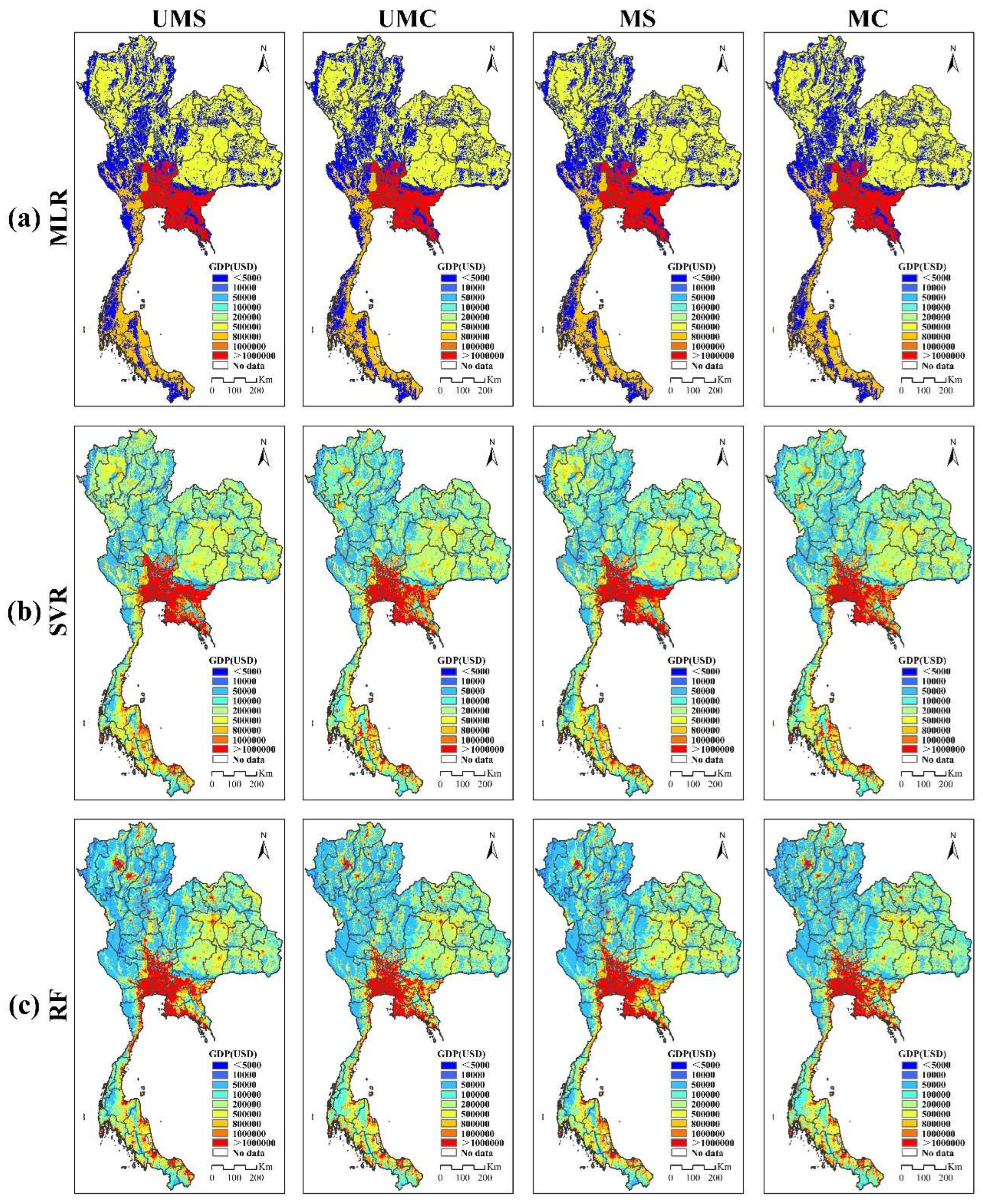
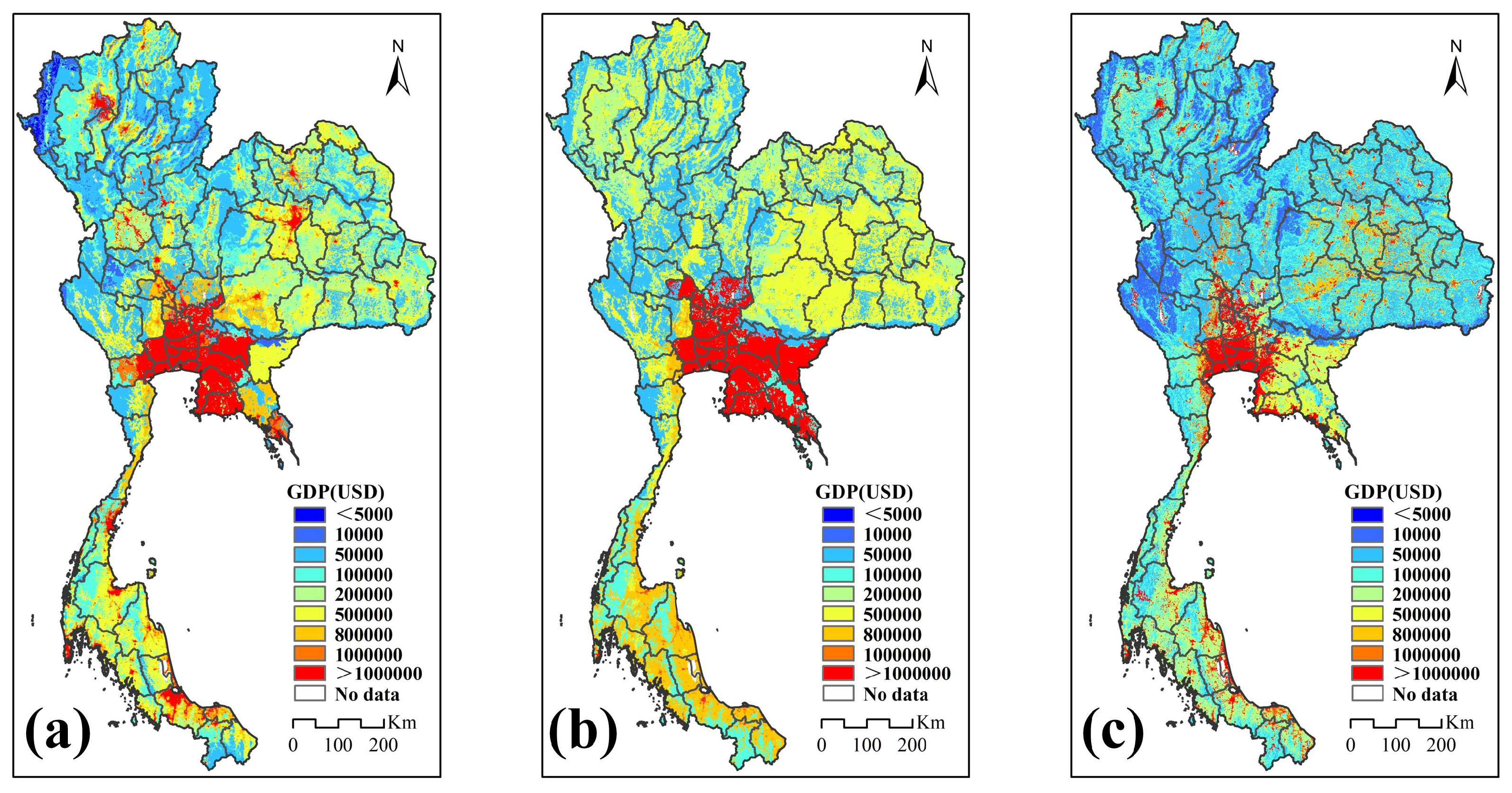
3.1. Gridded GDP Mapping

Depending on the categorization of the independent variables and the chosen method for spatializing GDP, a series of 1 km gridded GDP maps were generated, as visually represented in Figure 5 and Figure 6. In contrast to the statistical provincial GDP maps, which aggregate both agricultural and non-agricultural sectors (as illustrated in Figure 1c,d), the spatialized GDP maps provide a significantly finer-grained perspective by allocating GDP values within individual 1 km × 1 km grid cells. This approach affords an enhanced resolution, facilitating a more detailed examination of economic activities across the entire study area.

Evidently, the vicinity surrounding Bangkok emerged as the most economically developed region in Thailand, characterized by a robust business and industrial sector, consequently resulting in significantly elevated GDP values. This high GDP concentration in the Bangkok region was consistently reflected across all GDP downscaling predictions. However, the results obtained from the MLR and MLATARK methods exhibited notable disparities when compared to the outcomes derived from the other four machine learning-based methods. At the same time, the MLR and MLATARK methods had limitations in accurately representing GDP information for cities located beyond the provincial boundaries surrounding the capital. They struggled to effectively capture other economically developed regions. In contrast, the four machine learning-based methods demonstrated a superior ability to capture the major urban structures in economically prosperous provinces outside the capital, such as Songkhla, Phuket, Chiang Mai, Khon Kaen, Nakhon Ratchasima, and Kamphaeng Phet. In addition, variations in the selection of auxiliary variables also exerted a discernible influence on the spatial distribution of GDP. For instance, within the same modeling method, the utilization of different auxiliary variables led to conspicuous disparities in prediction outcomes, particularly in the periphery of the capital economic zone.

The influence of residual redistribution on the spatial distribution of GDP becomes evident through a comparative analysis of Figure 5 and Figure 6. As a consequence of this redistribution process, notable alterations in GDP values were observed in several provinces located outside the economic core centered around the capital, such as Sa Kaeo, Chanthaburi, Trat, Chai Nat, and Ratchaburi. Moreover, this redistribution of residuals induced significant transformations in the spatial distribution of GDP within the regions characterized by varying levels of economic development. For example, in the SVATARK results, certain economically developed areas experienced an increase in GDP values, while certain less developed areas witnessed a decrease. Conversely, RFATARK’s results reveal a decrease in GDP values within specific economically developed regions, coupled with a simultaneous increase in GDP values within certain less developed areas.

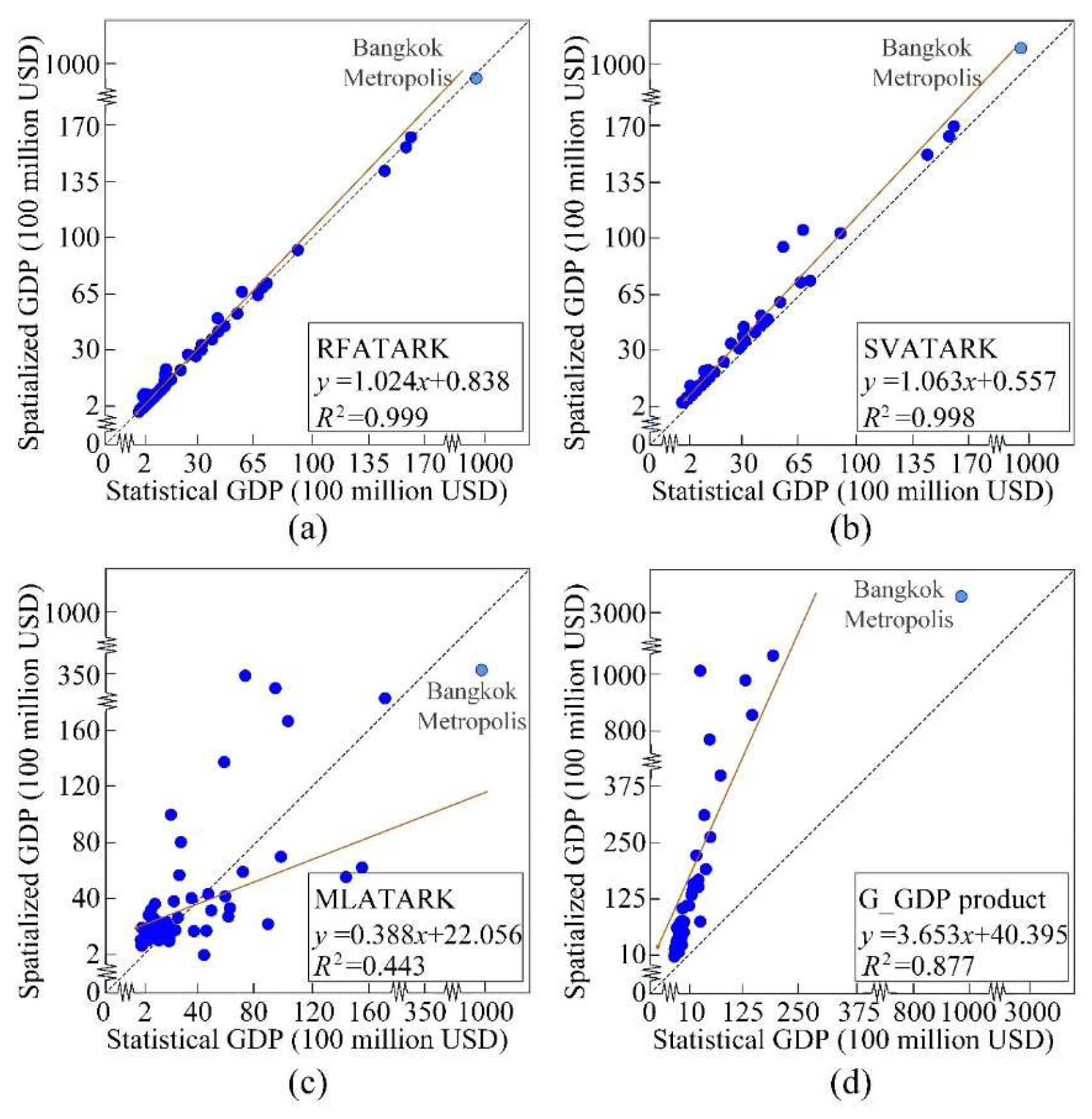
3.2. Accuracy Assessment

The spatialization of GDP results was carried out utilizing various models based on four groups of auxiliary variables, namely UMS, UMC, MS, and MC. These predictions were aggregated to the administrative province level. The accuracy of these downscaled results was subsequently validated using provincial GDP data. Additionally, a comparison was made with an existing gridded GDP product referred to as G_GDP.

Table 4. Performance of the different models based on three statistical measures between the estimated and actual GDP in province level. The RMSE and MAE values are in 10⁷ USD. Bolding indicates the situation with the highest precision.

Model	Category	RMSE	MAE	R2
RF	UMS	7550.438	2198.005	0.578
	UMC	7093.521	2124.864	0.642
	MS	7431.198	2163.931	0.598
	MC	7065.877	2107.321	0.647
	Average	7285.259	2148.53	0.616
SVR	UMS	8756.371	2597.505	0.391
	UMC	8424.893	2464.847	0.443
	MS	8747.029	2559.936	0.393
	MC	8414.596	2461.994	0.445
	Average	8585.722	2521.071	0.418
MLR	UMS	17,259.112	4397.361	0.551
	UMC	16,309.466	4695.980	0.363
	MS	51,242.087	13,478.187	0.607
	MC	184,033.264	40,547.569	0.611
	Average	67,210.980	15,779.77	0.533
RFATARK	UMS	987.344	326.345	0.981
	UMC	987.006	328.335	0.965
	MS	420.958	196.956	0.993
	MC	402.082	174.195	0.998
	Average	699.348	256.458	0.984
SVATARK	UMS	1031.165	294.517	0.972
	UMC	1027.465	297.735	0.998
	MS	936.841	308.826	0.977
	MC	915.298	288.899	0.996
	Average	977.692	297.494	0.986
MLATARK	UMS	9174.452	2782.196	0.328
	UMC	8771.900	2704.327	0.388
	MS	9159.387	2779.289	0.331
	MC	8363.801	2621.250	0.451
	Average	8867.385	2721.766	0.375
G_GDP	/	36,042.271	13,657.988	0.877

presents a comprehensive evaluation of the model performances, utilizing three classical statistical metrics.

Among the three methods that do not incorporate residual redistribution, the RF models consistently demonstrated strong predictive capabilities across different categories. For both UMS and UMC, RF achieved an average RMSE of approximately 7322.48. Similarly, in the case of MS and MC, RF maintained consistently relatively low RMSE values, averaging around 7248.037. This accuracy was further substantiated by the models’ performance, with an average MAE of approximately 2148.53. While the SVR models were competitive, they slightly trailed behind RF. In both the UMS and UMC, SVR achieved an average RMSE of approximately 8590.632, whereas in MS and MC, SVR maintained a comparable RMSE of approximately 8593.313. The SVR models exhibited an average MAE of approximately 2521.071, reflecting their overall accuracy. On the other hand, the MLR models yielded mixed results. In the UMS and UMC categories, MLR achieved moderate predictive accuracy, with an average RMSE of approximately 12,974.289. However, in the MS and MC categories, MLR’s accuracy significantly declined, resulting in an average RMSE of approximately 42,859.676. The MLR models exhibited an average MAE of approximately 15,779.77.

Comparatively, the method incorporating residual redistribution led to a substantial reduction in the mean RMSE and MAE when compared to the method without such a redistribution. Moreover, the residual redistribution method notably enhanced the mean R² in the machine learning-based models, although this improvement was not observed in the case of MLR. Overall, the models with residual redistribution outperform those without, underscoring the advantages of incorporating residual redistribution methods. Specifically, the RFATARK models exceled across all scenarios, consistently achieving remarkable precision with an average RMSE below 1000 and an average MAE of approximately 256.458. The SVATARK models also demonstrated strong predictive performance, with an average RMSE of approximately 977.692 and an average MAE of approximately 297.494. While RFATARK and SVATARK possessed similar mean R² values, RFATARK exhibited smaller mean RMSE and MAE values, suggesting its superiority in spatializing GDP. In contrast, the MLATARK models displayed relatively lower predictive accuracy, with an average RMSE ranging from approximately 8363.801 to 9174.452 across categories, and an average MAE of approximately 2721.766. As previously discussed, the RFATARK models consistently outperform other methods in terms of predictive accuracy. Notably, the RFATARK model, utilizing the MC group of auxiliary variables, achieved the highest accuracy among all scenarios, with an RMSE value of 402.082, a MAE value of 174.195, and an R² value of 0.998. Furthermore, comparing the prediction results of different independent variable groups, it is evident that, apart from the MLR-based method, the classification and factor weighting of OSM variables significantly enhance prediction accuracy.

To further validate the model performances, we compared the RFATARK, SVATARK, and MLATARK results within the MC group with G_GDP using scatter plots (Figure 7). The linearity of RFATARK and SVATARK with statistical GDP is notably superior to that of MLATARK and G_GDP, as evidenced by R² values of 0.999, 0.998, 0.443, and 0.877 for RFATARK, SVATARK, MLATARK, and G_GDP, respectively. Additionally, the regression lines for RFATARK and SVATARK closely align with the 1:1 line when compared with statistical GDP, as indicated by the slope of the regression line. Specifically, the slopes of the regression lines for RFATARK, SVATARK, MLATARK, and G_GDP were 1.024, 1.063, 0.388, and 3.653, respectively. In comparison to SVATARK, RFATARK demonstrated the advantage of a slope closer to 1, making it better suited for predicting GDP in economically developed regions, such as Bangkok and its surrounding provinces.

4. Discussion

Gridded GDP data with fine spatial resolution are invaluable for offering detailed insights into the spatial distribution of GDP, facilitating comprehensive socio-economic analyses alongside other rasterized geoscientific big data. In this study, we introduced a hybrid GDP spatialization approach that integrates random forest and geostatistical analysis to downscale statistical GDP data into gridded GDP data, leveraging a diverse range of geospatial big data sources. The trajectory of research in GDP spatialization methods has witnessed a shift from modeling total GDP to sector-specific GDP, from reliance solely on NTL data to incorporating broader geoscientific big data, and from linear GDP prediction models to more sophisticated counterparts. We explored the effects of residual redistribution on prediction accuracy and considered the influence of various potential factors on the accuracy of predictions.

4.1. GDP Spatialization for Different Sectors

In contrast to the traditional approach of directly modeling total GDP, we have chosen to separately simulate agricultural GDP and non-agricultural GDP. Historically, NTL data exhibit a strong linear relationship with total GDP, serving as a foundational element for spatializing total GDP [7,23]. However, it became evident that the accuracy of linear models for total GDP is significantly influenced by the dominant GDP sector [23]. Consequently, scholars increasingly began optimizing GDP spatialization results by developing models for different GDP sectors.

Early investigations suggested that the latitude and the variation coefficient of NTL could be leveraged to partition GDP into agricultural and non-agricultural components, thereby paving the way for future studies [56,57]. While some studies have employed NTL data, gridded population data, and the fraction of primary sector GDP in the total GDP of each statistical unit to spatialize primary sector GDP (e.g., agricultural or rural GDP), the varying relationship between population and primary sector GDP within this sector has posed challenges and introduced systematic errors into the results of GDP spatialization.

More recent studies have capitalized on LULC data in conjunction with NTL data to spatialize GDP across different sectors [6,15,24,25,32]. This approach allows for the refinement of GDP models for specific sectors, resulting in more realistic GDP distributions. For instance, Chen et al. [34] introduced distinct GDP models for six sectors, four of which fall within the primary sector, while Ustaoglu et al. [33] advocated for the inclusion of vegetation indices in the GDP prediction model to optimize GDP spatialization results. In our study, we combined the strengths of both approaches, considering the robust relationship between population and primary sector GDP while also using LULC data to refine the GDP prediction model. Nevertheless, we chose not to further subdivide GDP into additional sectors due to computational efficiency considerations, as separating secondary and tertiary sectors presents challenges [34].

4.2. Data Used for GDP Spatialization

This study incorporated a wide array of geoscientific data types in GDP spatialization, as illustrated in Table 1, Table 2 and Table 3. Early efforts in GDP spatialization primarily relied on statistical GDP data and NTL data [23,36]. This approach was often employed to investigate factors influencing the relationship between NTL and GDP, such as temporal effects [16,22]. However, this method faced limitations when spatializing GDP at scales smaller than the smallest statistical unit, such as at the pixel level. This limitation prompted our utilization of a broader array of geoscientific big data, in addition to NTL data.

Supplementing NTL data with other datasets has become commonplace to enhance GDP mapping for different sectors. The strong correlation between population data and agricultural GDP has led researchers to incorporate gridded demographic data, particularly when spatializing agricultural GDP [19,26,29]. Additional data often used alongside population data includes settlement patterns, primary sector GDP contributions to total GDP, agricultural product prices, and geographical coordinates [31,58]. Location information, encompassing latitude, longitude, and altitude, is also a common auxiliary variable in GDP spatialization [15,27,34,56], with evidence demonstrating the significant influence of geomorphological types detected through altitude on GDP [13]. Furthermore, LULC data have frequently been used alongside NTL data for GDP spatialization [24,25,28,32]. Specifically, when spatializing agricultural GDP, LULC data have been combined with vegetation indices such as EVI, NDVI, or net primary productivity (NPP) [6,33,34]. Recent research in GDP spatialization has incorporated an array of geoscientific big data, including road networks, building information, POIs, and more [15,27,34].

In our study, we employed NTL data, population data, terrain information, LULC data, vegetation indices, LST, road and water information, and POI data to spatialize GDP. The incorporation of diverse geoscientific data sources enables the generation of a more accurate gridded GDP map. However, it is essential to acknowledge that this approach entails challenges related to data acquisition and increased computational demands. Given the constraints of data availability, it is noteworthy that some auxiliary variables, as discussed above, were not utilized in the present experiment. Nevertheless, it is essential to underscore that these excluded variables remain viable candidates for incorporation in future GDP spatialization studies, with the potential to augment the precision of the final gridded GDP predictions, an avenue that merits further exploration. A noteworthy consideration is the observation that the population residing in one pixel may be involved in economic activities in another pixel. Consequently, datasets related to public utility (such as roads and water) and production factor (such as POIs) data may not fully capture the intricate dynamics of economic activity. To improve the practical relevance of the gridded GDP results in governance and business decision-making contexts, future GDP spatialization models could incorporate data specifically addressing the population engaged in economic activities. This approach may yield a more precise representation of the economic landscape by accounting for workforce distribution and employment patterns within distinct geographic units. Through the inclusion of data on the population actively contributing to economic productivity, the resulting gridded GDP model has the potential to provide insights more directly applicable to governmental policy formulation and enterprise-level decision-making processes.

Moreover, our study explores various combinations of auxiliary variables, yielding distinct groupings based on data processing, which are denoted as UMS, UMC, MS, and MC groups. Within these four distinct groups, the MC and MS groups exhibit the lowest number of variables, followed by the UMC group, while the UMS group boasts the highest number of variables. Notably, across different scaling experiments, the results obtained using the MC variable group consistently manifested superior accuracy. This observation underscores the notion that a greater abundance of auxiliary variables does not necessarily translate into heightened predictive accuracy. This phenomenon can be attributed, in part, to the possibility that the introduction of additional variables may amplify the impact of error, potentially outweighing their contribution to the modeling process. Conversely, the attribute integration process takes into consideration the unique characteristics of these variables, potentially leading to more accurate representations of their underlying conditions. For instance, by factoring in road network classifications and applying weighted integration techniques, we are able to capture a more precise overall depiction of the road network than would be achievable by analyzing each road network attribute in isolation.

4.3. GDP Spatialization Methods

Initially, GDP spatialization relied on linear models [7,23]. However, Ghosh et al. [29] highlighted the need to consider variations in the linear NTL-GDP relationship among administrative units. Simple linear models exhibited substantial GDP precision errors. To enhance accuracy, some scholars proposed using “lit-population,” calculated as the product of NTL and population, as an independent variable in linear models [26,58]. It is worth noting that simple linear models are ill-suited for simulating GDP across different sectors.

Building upon simple linear models, Doll et al. [10] introduced the log-linear model, later expanded by Henderson et al. [59], to incorporate cross-sectional and temporal effects. Additional models capable of disaggregating GDP into sectors, such as log-quadratic and multivariate log-linear models [19], have emerged. Zhang and Gibson [22] extended this framework to distinguish unobserved time-invariant features within cross-sectional units and spatially invariant features across time periods. While widely used to investigate NTL-GDP relationships, these models exhibit limitations in GDP spatialization accuracy.

Various regression models, including quadratic polynomial, power, exponential, stepwise multiple regression, multivariate linear regression, and fractional multivariate models, have demonstrated superior performance compared to simple linear models [6,13,24,27,33]. Notably, the latter three models incorporate not only NTL data but also diverse geographical data for GDP forecasting.

While the discussed models offer valuable insights, they fall under the category of traditional statistical approaches and have limitations. Recent advancements in GDP spatialization have seen the adoption of artificial intelligence algorithms, such as RF regression and deep learning models [15,27,34,49]. These intelligent models have demonstrated remarkable capabilities in simulating GDP, primarily attributed to their capacity to harness extensive geographical data and deploy sophisticated modeling techniques. However, it is essential to acknowledge a significant drawback associated with these artificial intelligence models—their ‘black box’ nature—which limits interpretability.

In our study, we adopted the RF regression model for GDP forecasting. Additionally, we introduced a hybrid approach involving the incorporation of a residual distribution based on geostatistical interpolation. Previous studies have utilized residuals solely to gauge model accuracy. Some of these studies, following accuracy assessments, applied residuals at the target spatial scale to attain unbiased results at the original spatial scale [27,33]. However, this residual distribution method merely corrects spatial residuals by adjusting the ratio of actual GDP to forecasted GDP, without accounting for the challenge posed by modifiable area units. In contrast, our method employs a geostatistical approach, known as ATAK, to effectively address the issue of modifiable area units, resulting in improved GDP spatialization outcomes compared to models lacking residual distribution.

4.4. Impact of Residual Predictions

In the introduction and the preceding section, we previously highlighted the potential enhancement in overall prediction accuracy through the integration of residual prediction. Due to the lack of detailed statistical GDP data at finer administrative levels, such as city and street-level GDP data in our experimental setup, we utilized the most detailed available provincial-level statistical GDP data for validation purposes. Considering that residual predictions were also based on the redistribution within provincial administrative units, theoretically, the validation of results at the provincial level, combined with residual predictions, should outperform downscaling models that do not consider residuals. This theoretical advantage is reflected in the results and comparative analysis. As indicated in the previous sections, the RFATARK method utilizing the auxiliary variables of MC group demonstrated the highest accuracy in downscaled GDP predictions. To further illustrate the superiority of the proposed RFATARK method, we conducted additional comparisons with three downscaling models under the MC auxiliary variable group. One model employed random forest inverse distance weighting (RFIDW), utilizing inverse distance weighting for residual redistribution. The other two models incorporated additional auxiliary variables into the random forest and XGBoost models (denoted as RF_MC and XGBoost), respectively, by adding latitude and longitude information into the MC auxiliary variable group. Figure 8 displays the downscaled GDP spatial distribution maps for these three methods, and

Table 5. Performance of the three downscaling models (including RFIDW, RF, and XGBoost) using MC group auxiliary variables. The RMSE and MAE values are in 10⁷ USD.

Model	RMSE	MAE	R2
RFIDW	1528.675	460.424	0.578
RF_MC	8673.488	2672.458	0.503
XGBoost	8679.099	2615.605	0.504

presents their accuracy assessment results.

In comparing modeling results employing different residual redistribution methods, the RFIDW model demonstrated relatively inferior performance compared to the RFA-TARK model. It exhibited an increased RMSE of approximately 1528.675 and an MAE of about 460.424, which are approximately three times higher than those of the RFATARK model. This demonstrates the higher predictive accuracy achieved by the downscaling model that integrates ATAK residual prediction. Regarding models incorporating latitude and longitude information without residuals, the RF model showed an RMSE of approximately 8673.488 and an MAE of 2672.458, while XGBoost exhibited an RMSE of about 8679.099 and an MAE of 2615.605. Both models displayed lower predictive accuracy than the RFATARK model. This is attributed to the fact that both RF and XGBoost were trained and established regression models at coarse resolutions, limiting their ability to capture GDP information at the target scale. Additionally, latitude and longitude generally represent the central position information of the corresponding unit, and from the provincial to kilometer grid, there is a significant difference in scale. Incorporating latitude and longitude as auxiliary variables did not significantly enhance predictive accuracy, and was particularly weaker than the benefits brought by the residual redistribution method. The integration of longitude and latitude into the residual-based downscaling method will be considered in future research to enhance predictive accuracy.

Furthermore, both RF and XGBoost belong to ensemble learning algorithms [60]. The former employs bagging, constructing multiple decision trees independently, and combining their predictions through averaging or voting. The latter utilizes a boosting-based ensemble technique, sequentially building trees, with each tree correcting the errors of the previous one. RF can employ bootstrapping to prevent model instability, while the XGBoost algorithm primarily penalizes the structure of decision trees to prevent overfit-ting. XGBoost often performs better in applications, but in some cases, the two show simi-lar performances [61,62,63]. Considering that RF is more user-friendly in terms of parameter tuning and less prone to overfitting than the XGBoost method [64], and given the moder-ate dataset used in our experiment, we proposed the RFATARK downscaling method which is a combination of RF and ATAK. In future applications, the XGBoost method can be integrated with ATAK residual prediction for downscaling, following the same steps as the RFATARK method but using the XGBoost method during regression modeling.

4.5. Additional Factors Potentially Impacting Accuracy

The accuracy of downscaling predictions is influenced by the model. In the process of downscaling modeling, it is commonly assumed that the model parameters of the target variable and auxiliary variables remain constant at both coarse and finer scales. However, due to the presence of scale effects, the relationship models between variables dynamically change with scale [65]. The greater the differences in scale, the poorer the applicability of the model may become. In this experiment, due to the lack of more detailed administrative units such as counties or streets in the statistical GDP data, provincial-level GDP statistical data were utilized for modeling. As there is a significant gap between the provincial level and the target scale of 1 km, the accuracy of the model may be compromised when applying the province-level GDP model to 1 km grids. Subsequently, in the process of correcting the model simulation results, as the remaining provincial data needs to be used as validation data, regional GDP statistics were employed for correction. The difference in scale between the regional level and the provincial level, as well as the kilometer grid scale, could have negative implications for result accuracy. In future research, obtaining statistical data at multiple scales would be advantageous for enhancing modeling effectiveness.

Additionally, the accuracy of variables involved in the modeling process also affects the accuracy of downscaling predictions. The errors in variables directly impact the modeling process and accumulate as the model progresses. On one hand, variables exhibit certain observation errors, and on the other hand, they have representativeness errors. In particular, for socio-economic variables, the current pixel-based partitioning (i.e., 1 km grids) may inadvertently lead to the truncation of certain production factors as they might be divided by pixel contours in space. This fragmentation of production factors could affect the accuracy of calculations, especially when attempting to capture the overall economic functions of a given spatial unit. In future research, it might be beneficial to consider using analysis units with greater spatial coherence to better capture subtle economic dynamics within each region. This approach could also provide a more realistic representation of the interconnections between economic factors that extend beyond pixel boundaries, thereby improving the overall accuracy and reliability of modeling results. For example, reorganizing pixels into larger, more coherent regions that serve as subdivisions of provinces could ensure spatial continuity of economic activities and allow for a more accurate description of the intricate relationships between production factors, providing a more realistic representation of the economic landscape within each region.

5. Conclusions

This paper introduced a hybrid GDP spatialization method, which employs a RF regression model in conjunction with the ATAK technique, and utilizes multi-source data as auxiliary information. The proposed approach entails the construction of distinct RF models for the agricultural and non-agricultural sectors, allowing us to capture the non-linear relationships between independent variables and the statistical GDP pertaining to diverse sectors. Subsequently, the application of ATAK facilitates the distribution of residuals in the GDP prediction process. This hybrid approach, which has not been extensively explored in previous GDP spatialization studies, plays a pivotal role in refining the spatial distribution of GDP predictions. The integration of diverse geoscientific data sources, coupled with the proposed methodological framework, has yielded significant improvements in the predictive capabilities of GDP spatialization. Our case study focusing on Thailand’s GDP underscores the efficacy of our approach, providing a more accurate and intuitive visualization of GDP distribution. Additionally, we have examined the utility of four distinct sets of covariates in the downscaling process, with the MC group demonstrating superior informativeness compared to the UMS, UMC, and MS groups, thereby yielding the most accurate downscaled predictions. The methodology introduced in this study can be extended to downscale GDP data for additional time periods, as well as to finer resolution grids, through the incorporation of auxiliary information corresponding to the desired resolution. The resulting gridded GDP map serves as a valuable scientific resource for government bodies and organizations, facilitating the formulation of informed development strategies.

References

1. Liu, Z.; He, C.; Zhang, Q.; Huang, Q.; Yang, Y. Extracting the Dynamics of Urban Expansion in China Using DMSP-OLS Nighttime Light Data from 1992 to 2008. Landsc. Urban Plan. 2012, 106, 62–72. [Google Scholar] [CrossRef]
2. Jean, N.; Burke, M.; Xie, M.; Davis, W.M.; Lobell, D.B.; Ermon, S. Combining Satellite Imagery and Machine Learning to Predict Poverty. Science 2016, 353, 790–794. [Google Scholar] [CrossRef] [PubMed]
3. Zhao, N.; Currit, N.; Samson, E. Net Primary Production and Gross Domestic Product in China Derived from Satellite Imagery. Ecol. Econ. 2011, 70, 921–928. [Google Scholar] [CrossRef]
4. Zhao, S.; Liu, Y.; Zhang, R.; Fu, B. China’s Population Spatialization Based on Three Machine Learning Models. J. Clean. Prod. 2020, 256, 120644. [Google Scholar] [CrossRef]
5. Li, F.; Mi, X. Spatialization of GDP in Beijing Using NPP-VIIRS Data. Remote Sens. Nat. Resour. 2016, 28, 19–24. [Google Scholar] [CrossRef]
6. Yue, W.; Gao, J.; Yang, X. Estimation of Gross Domestic Product Using Multi-Sensor Remote Sensing Data: A Case Study in Zhejiang Province, East China. Remote Sens. 2014, 6, 7260–7275. [Google Scholar] [CrossRef]
7. Elvidge, C.D.; Baugh, K.E.; Kihn, E.A.; Kroehl, H.W.; Davis, E.R.; Davis, C.W. Relation between Satellite Observed Visible-near Infrared Emissions, Population, Economic Activity and Electric Power Consumption. Int. J. Remote Sens. 1997, 18, 1373–1379. [Google Scholar] [CrossRef]
8. Huang, Q.; Yang, X.; Gao, B.; Yang, Y.; Zhao, Y. Application of DMSP/OLS Nighttime Light Images: A Meta-Analysis and a Systematic Literature Review. Remote Sens. 2014, 6, 6844–6866. [Google Scholar] [CrossRef]
9. Bennett, M.M.; Smith, L.C. Advances in Using Multitemporal Night-Time Lights Satellite Imagery to Detect, Estimate, and Monitor Socioeconomic Dynamics. Remote Sens. Environ. 2017, 192, 176–197. [Google Scholar] [CrossRef]
10. Doll, C.H.; Muller, J.-P.; Elvidge, C.D. Night-Time Imagery as a Tool for Global Mapping of Socioeconomic Parameters and Greenhouse Gas Emissions. Ambio 2000, 29, 157–162. [Google Scholar] [CrossRef]
11. Elvidge, C.D.; Zhizhin, M.; Hsu, F.-C.; Baugh, K.E. VIIRS Nightfire: Satellite Pyrometry at Night. Remote Sens. 2013, 5, 4423–4449. [Google Scholar] [CrossRef]
12. Zhao, M.; Zhou, Y.; Li, X.; Cao, W.; He, C.; Yu, B.; Li, X.; Elvidge, C.D.; Cheng, W.; Zhou, C. Applications of Satellite Remote Sensing of Nighttime Light Observations: Advances, Challenges, and Perspectives. Remote Sens. 2019, 11, 1971. [Google Scholar] [CrossRef]
13. Zhao, M.; Cheng, W.; Zhou, C.; Li, M.; Wang, N.; Liu, Q. GDP Spatialization and Economic Differences in South China Based on NPP-VIIRS Nighttime Light Imagery. Remote Sens. 2017, 9, 673. [Google Scholar] [CrossRef]
14. Elvidge, C.D.; Zhizhin, M.; Ghosh, T.; Hsu, F.-C.; Taneja, J. Annual Time Series of Global VIIRS Nighttime Lights Derived from Monthly Averages: 2012 to 2019. Remote Sens 2021, 13, 922. [Google Scholar] [CrossRef]
15. Chen, Y.; Wu, G.; Ge, Y.; Xu, Z. Mapping Gridded Gross Domestic Product (GDP) Distribution of China Using Deep Learning With Multiple Geospatial Big Data. IEEE J. Sel. Top. Appl. Earth Obs. Remote Sens. 2022, 15, 1791–1802. [Google Scholar] [CrossRef]
16. Gibson, J.; Boe-Gibson, G. Nighttime Lights and County-Level Economic Activity in the United States: 2001 to 2019. Remote Sens. 2021, 13, 2741. [Google Scholar] [CrossRef]
17. Hutasavi, S.; Chen, D. Estimating District-Level Electricity Consumption Using Remotely Sensed Data in Eastern Economic Corridor, Thailand. Remote Sens. 2021, 13, 4654. [Google Scholar] [CrossRef]
18. Hutasavi, S.; Chen, D. Exploring the Industrial Growth and Poverty Alleviation through Space-Time Data Mining from Night-Time Light Images: A Case Study in Eastern Economic Corridor (EEC), Thailand. Int. J. Remote Sens. 2022, 1–23. [Google Scholar] [CrossRef]
19. McCord, G.C.; Rodriguez-Heredia, M. Nightlights and Subnational Economic Activity: Estimating Departmental GDP in Paraguay. Remote Sens. 2022, 14, 1150. [Google Scholar] [CrossRef]
20. Pérez-Sindín, X.S.; Chen, T.-H.K.; Prishchepov, A.V. Are Night-Time Lights a Good Proxy of Economic Activity in Rural Areas in Middle and Low-Income Countries? Examining the Empirical Evidence from Colombia. Remote Sens. Appl. 2021, 24, 100647. [Google Scholar] [CrossRef]
21. Weidmann, N.B.; Theunissen, G. Estimating Local Inequality from Nighttime Lights. Remote Sens. 2021, 13, 4624. [Google Scholar] [CrossRef]
22. Zhang, X.; Gibson, J. Using Multi-Source Nighttime Lights Data to Proxy for County-Level Economic Activity in China from 2012 to 2019. Remote Sens. 2022, 14, 1282. [Google Scholar] [CrossRef]
23. Doll, C.N.H.; Muller, J.-P.; Morley, J.G. Mapping Regional Economic Activity from Night-Time Light Satellite Imagery. Ecol. Econ. 2006, 57, 75–92. [Google Scholar] [CrossRef]
24. Han, X.; Zhou, Y.; Wang, S.; Liu, R.; Yao, Y. GDP Spatialization in China Based on Nighttime Imagery. Geo-Inf. Sci. 2012, 14, 128–136. [Google Scholar] [CrossRef]
25. Chen, Q.; Hou, X.; Zhang, X.; Ma, C. Improved GDP Spatialization Approach by Combining Land-Use Data and Night-Time Light Data: A Case Study in China’s Continental Coastal Area. Int. J. Remote Sens. 2016, 37, 4610–4622. [Google Scholar] [CrossRef]
26. Zhao, N.; Liu, Y.; Cao, G.; Samson, E.L.; Zhang, J. Forecasting China’s GDP at the Pixel Level Using Nighttime Lights Time Series and Population Images. GIsci Remote Sens. 2017, 54, 407–425. [Google Scholar] [CrossRef]
27. Liang, H.; Guo, Z.; Wu, J.; Chen, Z. GDP Spatialization in Ningbo City Based on NPP/VIIRS Night-Time Light and Auxiliary Data Using Random Forest Regression. Adv. Space Res. 2020, 65, 481–493. [Google Scholar] [CrossRef]
28. Sun, J.; Di, L.; Sun, Z.; Wang, J.; Wu, Y. Estimation of GDP Using Deep Learning With NPP-VIIRS Imagery and Land Cover Data at the County Level in CONUS. IEEE J. Sel. Top. Appl. Earth Obs. Remote Sens. 2020, 13, 1400–1415. [Google Scholar] [CrossRef]
29. Ghosh, T.; Powell, R.L.; Elvidge, C.D.; Baugh, K.E.; Sutton, P.C.; Anderson, S. Shedding Light on the Global Distribution of Economic Activity. Open Geogr. J. 2010, 3, 147–160. [Google Scholar] [CrossRef]
30. Li, G.; Fang, C. Global Mapping and Estimation of Ecosystem Services Values and Gross Domestic Product: A Spatially Explicit Integration of National ‘Green GDP’ Accounting. Ecol. Indic. 2014, 46, 293–314. [Google Scholar] [CrossRef]
31. Wang, X.; Rafa, M.; Moyer, J.D.; Li, J.; Scheer, J.; Sutton, P. Estimation and Mapping of Sub-National GDP in Uganda Using NPP-VIIRS Imagery. Remote Sens. 2019, 11, 163. [Google Scholar] [CrossRef]
32. Keola, S.; Andersson, M.; Hall, O. Monitoring Economic Development from Space: Using Nighttime Light and Land Cover Data to Measure Economic Growth. World Dev. 2015, 66, 322–334. [Google Scholar] [CrossRef]
33. Ustaoglu, E.; Bovkır, R.; Aydınoglu, A.C. Spatial Distribution of GDP Based on Integrated NPS-VIIRS Nighttime Light and MODIS EVI Data: A Case Study of Turkey. Environ. Dev. Sustain. 2021, 23, 10309–10343. [Google Scholar] [CrossRef]
34. Chen, Q.; Ye, T.; Zhao, N.; Ding, M.; Ouyang, Z.; Jia, P.; Yue, W.; Yang, X. Mapping China’s Regional Economic Activity by Integrating Points-of-Interest and Remote Sensing Data with Random Forest. Environ. Plan. B Urban. Anal. City Sci. 2021, 48, 1876–1894. [Google Scholar] [CrossRef]
35. Sutton, P.C.; Costanza, R. Global Estimates of Market and Non-Market Values Derived from Nighttime Satellite Imagery, Land Cover, and Ecosystem Service Valuation. Ecol. Econ. 2002, 41, 509–527. [Google Scholar] [CrossRef]
36. Sutton, P.; Elvidge, C.; Tilottama, G. Estimation of Gross Domestic Product at Sub-National Scales Using Nighttime Satellite Imagery. Int. J. Ecol. Econ. Stat. 2007, 8, 5–21. [Google Scholar]
37. Punyaratabandhu, P.; Swaspitchayaskun, J. The Political Economy of China–Thailand Development Under the One Belt One Road Initiative: Challenges and Opportunities. Chin. Econ. 2018, 51, 333–341. [Google Scholar] [CrossRef]
38. Apipattanavis, S.; Ketpratoom, S.; Kladkempetch, P. Water Management in Thailand. Irrig. Drain. 2018, 67, 113–117. [Google Scholar] [CrossRef]
39. Ariyapruchya, K.; Sanchez Martin, M.E.; Reungsri, T.; Luo, X. Publication: Thailand Economic Monitor, June 2016: Aging Society and Economy. 2016. Available online: http://hdl.handle.net/10986/24940 (accessed on 22 December 2022).
40. Wang, Z.; Schaaf, C.B.; Sun, Q.; Shuai, Y.; Román, M.O. Capturing Rapid Land Surface Dynamics with Collection V006 MODIS BRDF/NBAR/Albedo (MCD43) Products. Remote Sens. Environ. 2018, 207, 50–64. [Google Scholar] [CrossRef]
41. Badgley, G.; Field, C.B.; Berry, J.A. Canopy Near-Infrared Reflectance and Terrestrial Photosynthesis. Sci. Adv. 2017, 3, e1602244. [Google Scholar] [CrossRef] [PubMed]
42. Huete, A.; Didan, K.; Miura, T.; Rodriguez, E.P.; Gao, X.; Ferreira, L.G. Overview of the Radiometric and Biophysical Performance of the MODIS Vegetation Indices. Remote Sens. Environ. 2002, 83, 195–213. [Google Scholar] [CrossRef]
43. Wan, Z. New Refinements and Validation of the Collection-6 MODIS Land-Surface Temperature/Emissivity Product. Remote Sens. Environ. 2014, 140, 36–45. [Google Scholar] [CrossRef]
44. Li, C.; Gong, P.; Wang, J.; Zhu, Z.; Biging, G.S.; Yuan, C.; Hu, T.; Zhang, H.; Wang, Q.; Li, X.; et al. The First All-Season Sample Set for Mapping Global Land Cover with Landsat-8 Data. Sci. Bull. 2017, 62, 508–515. [Google Scholar] [CrossRef] [PubMed]
45. Tachikawa, T.; Hato, M.; Kaku, M.; Iwasaki, A. Characteristics of ASTER GDEM Version 2. In Proceedings of the 2011 IEEE International Geoscience and Remote Sensing Symposium, Vancouver, BC, Canada, 24–29 July 2011; IEEE: Vancouver, BC, Canada, 2011; pp. 3657–3660, ISBN 978-1-4577-1005-6. [Google Scholar]
46. Kummu, M.; Taka, M.; Guillaume, J.H.A. Gridded Global Datasets for Gross Domestic Product and Human Development Index over 1990–2015. Sci. Data 2018, 5, 180004. [Google Scholar] [CrossRef] [PubMed]
47. Tatem, A.J. WorldPop, Open Data for Spatial Demography. Sci. Data 2017, 4, 170004. [Google Scholar] [CrossRef] [PubMed]
48. Wang, Y.; Huang, C.; Zhao, M.; Hou, J.; Zhang, Y.; Gu, J. Mapping the Population Density in Mainland China Using NPP/VIIRS and Points-Of-Interest Data Based on a Random Forests Model. Remote Sens. 2020, 12, 3645. [Google Scholar] [CrossRef]
49. Sun, M.; Wang, T.; Xu, X.; Zhang, L.; Li, J.; Shi, Y. Ecological Risk Assessment of Soil Cadmium in China’s Coastal Economic Development Zone: A Meta-Analysis. Ecosyst. Health Sustain. 2020, 6, 1733921. [Google Scholar] [CrossRef]
50. Breiman, L. Random Forests. Mach. Learn. 2001, 45, 5–32. [Google Scholar] [CrossRef]
51. Cutler, A.; Stevens, J.R. Random Forests for Microarrays. Methods Enzymol. 2006, 411, 422–432. [Google Scholar] [CrossRef]
52. Ham, J.; Chen, Y.; Crawford, M.M.; Ghosh, J. Investigation of the Random Forest Framework for Classification of Hyperspectral Data. IEEE Trans. Geosci. Remote Sens. 2005, 43, 492–501. [Google Scholar] [CrossRef]
53. Goovaerts, P. Kriging and Semivariogram Deconvolution in the Presence of Irregular Geographical Units. Math. Geosci. 2008, 40, 101–128. [Google Scholar] [CrossRef]
54. Jin, Y.; Ge, Y.; Liu, Y.; Chen, Y.; Zhang, H.; Heuvelink, G.B.M. A Machine Learning-Based Geostatistical Downscaling Method for Coarse-Resolution Soil Moisture Products. IEEE J. Sel. Top. Appl. Earth Obs. Remote Sens. 2021, 14, 1025–1037. [Google Scholar] [CrossRef]
55. Smola, A.J.; Schölkopf, B. A Tutorial on Support Vector Regression. Stat. Comput. 2004, 14, 199–222. [Google Scholar] [CrossRef]
56. Wu, J. Landscape Sustainability Science: Ecosystem Services and Human Well-Being in Changing Landscapes. Landscape Ecol. 2013, 28, 999–1023. [Google Scholar] [CrossRef]
57. Wu, J.; Wang, Z.; Li, W.; Peng, J. Exploring Factors Affecting the Relationship between Light Consumption and GDP Based on DMSP/OLS Nighttime Satellite Imagery. Remote Sens. Environ. 2013, 134, 111–119. [Google Scholar] [CrossRef]
58. Wang, X.; Sutton, P.C.; Qi, B. Global Mapping of GDP at 1 Km2 Using VIIRS Nighttime Satellite Imagery. ISPRS Int. J. Geoinf. 2019, 8, 580. [Google Scholar] [CrossRef]
59. Henderson, J.V.; Storeygard, A.; Weil, D.N. Measuring Economic Growth from Outer Space. Am. Econ. Rev. 2012, 102, 994–1028. [Google Scholar] [CrossRef]
60. Natras, R.; Soja, B.; Schmidt, M. Ensemble Machine Learning of Random Forest, AdaBoost and XGBoost for Vertical Total Electron Content Forecasting. Remote Sens. 2022, 14, 3547. [Google Scholar] [CrossRef]
61. Zamani Joharestani, M.; Cao, C.; Ni, X.; Bashir, B.; Talebiesfandarani, S. PM2.5 Prediction Based on Random Forest, XGBoost, and Deep Learning Using Multisource Remote Sensing Data. Atmosphere 2019, 10, 373. [Google Scholar] [CrossRef]
62. Yu, J.-W.; Yoon, Y.-W.; Baek, W.-K.; Jung, H.-S. Forest Vertical Structure Mapping Using Two-Seasonal Optic Images and LiDAR DSM Acquired from UAV Platform through Random Forest, XGBoost, and Support Vector Machine Approaches. Remote Sens. 2021, 13, 4282. [Google Scholar] [CrossRef]
63. Wang, S.; Zhuang, J.; Zheng, J.; Fan, H.; Kong, J.; Zhan, J. Application of Bayesian hyperparameter optimized random forest and XGBoost model for landslide susceptibility mapping. Front. Earth Sci. 2021, 9, 712240. [Google Scholar] [CrossRef]
64. Kiangala, S.K.; Wang, Z.H. An effective adaptive customization framework for small manufacturing plants using extreme gradient boosting-XGBoost and random forest ensemble learning algorithms in an Industry 4.0 environment. Mach. Learn. Appl. 2021, 4, 100024. [Google Scholar] [CrossRef]
65. Ge, Y.; Jin, Y.; Stein, A.; Chen, Y.; Wang, J.; Wang, J.; Cheng, Q.; Bai, H.; Liu, M.; Atkinson, P.M. Principles and Methods of Scaling Geospatial Earth Science Data. Earth-Sci. Rev. 2019, 197, 102897. [Google Scholar] [CrossRef]
Figure 1. Elevation and regional divisions (a), LULC (b), agriculture statistical GDP (c), and non-agriculture statistical GDP (d) of Thailand at the province level. (GDP in constant 2011 international USD).
Ijgi 12 00481 g001
Figure 2. The result of KDE bandwidth determination.
Ijgi 12 00481 g002
Figure 3. Tuning curves of random forest modeling for agricultural and non-agricultural GDP with four different scenarios. (The horizontal coordinate represents mtree).
Ijgi 12 00481 g003
Figure 4. Flowchart of the GDP spatialization.
Ijgi 12 00481 g004
Figure 5. The spatial distribution of downscaled GDP using RF, SVR, and MLR methods.
Ijgi 12 00481 g005
Figure 6. The spatial distribution of downscaled GDP by using RFATARK, SVATARK, and MLATARK methods.
Ijgi 12 00481 g006
Figure 7. The linear relationship between statistical GDP and spatialized GDP at the provincial scale. GDP derived by (a) RFATARK, (b) SVATARK, (c) MLATARK using MC group of auxiliary variables, and (d) G_GDP product. The black dashed line represents the 1:1 line, and the orange line represents the line fitted through the scatter points.
Ijgi 12 00481 g007
Figure 8. The spatial distribution of downscaled GDP by using (a) RFIDW, (b) RF_MC, and (c) XGBoost methods and MC group auxiliary variables.
Ijgi 12 00481 g008