Towards the Monitoring of Underground Caves Using Geomatics and Geophysical Techniques: 3D Analyses and Seismic Response

Abstract

Analyses of climate change, due to its impact not only on the weather and the environment but also on human health and life, are one of the most important study activities made in recent years. There is relatively high confidence that glacial melt and heavy rainfall events will continue to increase. These climate-related events carry a microseismic signature that can guide monitoring activities. In the last decade, there have been growing applications of long-term continuous ambient seismic noise systems to monitor landslides and potentially unstable rock sites. This work reports some of the activities made during a project performed under the Department of Excellence on Climate Change (2018–2022), funded by the Italian Ministry for University and Research (MUR), in order to improve environmental seismic analyses. The selected test site is the Bossea Cave (NW Italy), where two seismic stations were installed. The goals were to use these stations to understand and study climate change events above the Bossea Cave, analyzing the data from a geophysical and geomatics point of view. Starting with UAV flights and photogrammetric processing to obtain a 3D model of the cave, both ambient seismic noise and microseismicity analyses highlighted an important effect of air temperature and precipitation on the seismic response of the monitored rock mass overlying the Bossea Cave. In particular, a clear effect on the ambient seismic noise spectral content and the peak frequency of the microseismic events driven by temperature and precipitation was found during the warmer monitoring months, with almost zero delays in the seismic response. This is a preliminary but important study, even if longer monitoring data and thermal modeling efforts are needed to fully understand this seasonal variation.

1. Introduction

In the last decade, several case studies of ambient seismic noise and microseismicity monitoring have been reported at different scales for landslide characterization and monitoring, hydrogeological assessments, fluvial seismology, short- and long-term monitoring of buildings, infrastructures and glacial bodies (e.g., [1,2,3]). In general, continuous passive seismic monitoring has created great interest in detecting and tracking the evolution of natural phenomena and anthropic structures as a function of the external forcing related to air temperature, wind, rainfall, and snowfall modifications. This aspect becomes of utmost importance for the monitoring of landslides and potentially unstable rock masses, where ambient seismic noise and microseismicity analyses have proved able to detect seismic precursors to failure [4,5,6,7].

In unstable sites, the fundamental resonance frequency of the prone-to-fall compartment can be easily derived from the noise spectral content and tracked over time for early-warning purposes [8,9]. The detection of irreversible drops in the resonance frequency value can indeed be read as a precursor to failure [4,7].

In parallel, the continuous ambient seismic noise record can contain impulsive events related to incipient fracturing, also called microseismic events. An increasing number of microseismic events is expected towards failure due to fracture propagation and growth (Amitrano et al., 2005 [10].). The microseismicity can consequently be tracked in time as a further and early-warning parameter.

In addition to the recognition of failure precursors, all the literature case studies on potentially unstable rock masses have also highlighted significant reversible modifications in the seismic parameters driven by thermo- and hydro-mechanical processes acting at the daily and seasonal scale 3. These reversible modifications help in understanding the rock mass behavior in response to the external forcing, that is changing in response to climate modifications. A variation in the rate or intensity of these thermo- and hydro-mechanical processes is likely a consequence of the ongoing climate change. For these reasons, passive seismic monitoring can offer valuable tools to investigate the possible modification of rock masses’ sensitivity to the external changing conditions.

While the ability of ambient seismic noise and microseismicity studies to measure and forecast the reaction of landslides and rock masses to external meteorological factors has been demonstrated in several case studies, little attention has been devoted to the study and monitoring of stable rock masses and other geological underground features, such as natural caves. Despite the absence of similar applications, seismic parameters might be useful to understand the evolution and inner dynamics of these targets and to forecast and locate possible instabilities related to the external forcing factors.

This work focuses on the study of the Bossea Cave (SW Italian Alps) by means of a first survey campaign based on geomatics and geophysical techniques for the reconstruction of a 3D model of the slope overlying the cave and the monitoring of the seasonal seismic response of the rock mass in relation to air temperature and precipitation. Every time we perform analyses, the localization of the site the data was collected from is mandatory. Thus, in order to georeference the positions of the geophysical samples, a geomatic survey was considered. As one of the goals was to locate the seismic analyses, a complete survey involving indoor and outdoor 3D reconstructions was made, guaranteeing the possibility of having every measurement placed in a correct way and connecting the indoor environment with the outdoor one.

In the cave, an underground laboratory was installed during the years 1969–1972 by a group of volunteer cavers of the speleological group “Alpi Marittime” of the Italian Alpine Club (CAI) of Cuneo [11]. This laboratory has been increasingly equipped over the years, progressively carrying out scientific research thanks to the continuous financial support of public administrations. In parallel, collaborations have started, initially with the “Dipartimento di Ingegneria dell’Ambiente, del Territorio e delle Infrastrutture” (DIATI) of the Politecnico di Torino, and later also with the Environmental Protection Agency (ARPA Piemonte) of Cuneo, and the Department Radiation of ARPA Valle d’Aosta. Other literature studies have already produced positive and constructive data analysis on this site [12,13].

This work encompasses two different approaches: geomatics characterization and geophysical monitoring. From the geomatics approach, the goal was to define a 3D model of the area around the cave. Based on the geomatics results, preliminary geophysical monitoring was developed for the site by means of two temporary passive seismic stations. Data integration, together with the analysis of the available meteorological data for the area, provides a good initial starting point for the understanding of the seasonal variability in the rock mass seismic response due to temperature and precipitation changes.

2. Case Study

The term cave refers to any type of underground cavity, whether natural or artificial, and which may have very variable morphology. Caves can be small and shallow or extend for kilometers, with length increasing or not in parallel levels or in branches. They can have a mainly horizontal or a vertical development. In Italy, about 35,000 caves are known with a length development of more than 5 m, for a total length development of about 2500 km of passages.

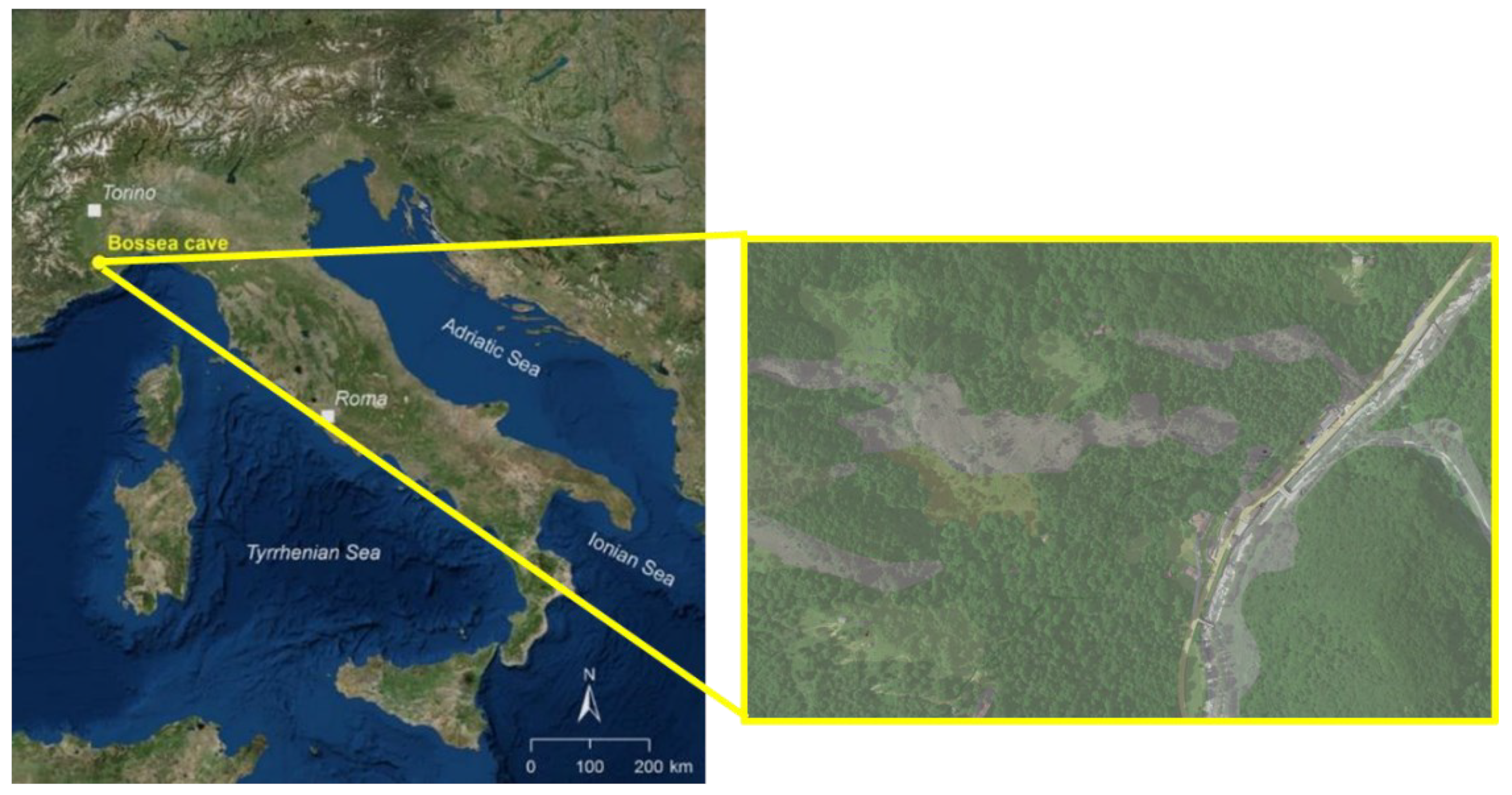
The area under investigation in this study is the Bossea Cave. It is located in Piedmont (Northwest of Italy); in particular, the area is in the valley of the Corsaglia stream in the province of Cuneo, about 110 km south from Turin (Figure 1).

The Bossea Cave is a natural karst cavity. Its origin can be linked to geological, chemical, and lithological features, and to hydrological phenomena of the region, particularly to the long-term effect of the surface and hypogeal circulation of water in carbonate rocks that are particularly predisposed to dissolution.

Discovered and explored in 1816, the cave was opened to the public on 2 August 1874. Moreover, since 1969 it has housed a karst laboratory (location in red in Figure 2) of the Italian Alpine Club, which investigates phenomena, including biological ones, still taking place in the cavity. The Bossea Cave, represented in Figure 2 through a mobile mapping indoor survey, was chosen for this study because it is an important environment that has recorded several variations in both its internal and external features related to temperature, precipitation and, in general, climate variations. This 3D survey was also helpful in individuating the slope of the cave and the main zones in which the water could erode the rocks.

In fact, it is actually one of the most important sites selected by the DIATI Department of Politecnico di Torino (Italy) to study climate change: the importance was also highlighted by a research project granted and funded by the Italian Ministry for University and Research (MUR), and performed under the Department of Excellence on Climate Change (2018–2022).

The cave constitutes the terminal sector of a large karst system that has developed in the Maudagna–Corsaglia watershed. The cave is divided into two zones: a lower area characterized by impressive large dimensions and an upper area consisting of a complex of narrow galleries developed on superimposed floors, with the two parts separated by the waterfall at Lake Ernestina. The lower area, about 900 m long and with an ascending difference in elevation of 116 m, is equipped for tourist visits and contains a stream whose flow rate varies from 50 to about 1500 L per second (Figure 3). To get an idea of the phenomena involved, note that the stream transports 5 million cubic meters of water every year, which contains an average of 50 mg/L of dissolved calcium carbonate for a total of 750 tons of rock removed annually from the karst system.

The origin of the Bossea Cave can be linked to geological, chemical, lithological, and hydrological phenomena of the region in which it was formed by the long-term effects of the surface- and, above all, hypogeal circulation of water. The water corrodes, dissolves and transports rocky material that is particularly predisposed to dissolution; in most cases, these are rocks of carbonate composition.

First, we defined what a karst cave is and its characteristics by evaluating its strengths and weaknesses, describing, in particular, the action of water, from sources to springs to aquifers. In karst rocks, the water is organized into water courses, sometimes real underground rivers, which can run through huge tunnels of several meters in diameter and up to several kilometers length development. The waters of underground courses move in the same way as surface water courses: like these, they are subject to floods caused by surface precipitation (which arrives in the cave with a certain delay, due to the slowness of infiltration). They can excavate and erode the rock with mechanical abrasion processes and carry sediments of various grain size and can create alluvial deposits inside the caves. The saturated zone of a karst system has a length development and a depth that depend on the geological structure: at times the saturated zone can be of very small thickness, or absent, as in karst systems “suspended” on the base level; at times it can be hundreds of meters thick and constitute an immense and precious water reserve. The most superficial zone of the saturated zone, called the epiphreatic zone, undergoes seasonal variations and can rise several tens of meters in the wettest periods: it is a very important zone for the formation of caves, because, thanks to the Boegli effect due to the mixing of waters with different chemical compositions (rainwater and deep waters), it is here that the largest galleries are formed (Figure 4). Below the epiphreatic zone, the waters of the saturated zone move very slowly and can remain within the karst aquifer for tens or hundreds of years, before emerging in springs. This means that karst waters are very vulnerable both to pollution (a pollutant could remain inside the aquifer for decades), and to excessive exploitation (the emptying of the saturated area could require decades for its refilling to the original level of waters): they are therefore precious reserves, but to be protected and exploited with great caution.

Furthermore, other aspects that we can introduce are the groundwater leaks to the surface that are called springs, where the origin of the water is unknown or comes from widespread absorption, or resurgences, if they are the outlet for water that goes underground at entrances further upstream. The springs can be classified in various ways, depending on the flow rate, the constancy of the flow or the geological characteristics that determine their formation.

3. Materials and Methods

In order to reach the goal and study the seasonal variability in the rock mass seismic response due to temperature and precipitation variations, both geomatics and geophysical techniques were employed. These activities are described hereinafter.

3.1. The Geomatics Tools

Two main approaches can be followed to perform the aerial photogrammetric acquisition properly: the so-called direct photogrammetry [14] or the use of Ground Control Points (GCPs). In the first case, the images are directly georeferenced from the information obtained through the accurate position of the center of the camera and the attitude angles. In the second case, it is mandatory to place some markers on the ground and to measure them through one or more geomatics techniques. As described in [15], GCPs are points with well-known coordinates (estimated with GNSS instruments in static or Real Time Kinematic—RTK, to reach accuracies of a few mm or cm, respectively), which are fundamental to constrain the aerial photogrammetric model for the 3D reconstruction. In the present work, the first approach was followed, according to the procedure reported in [16]. In particular, during the planning phase, it was highlighted that it was not possible to set markers on the ground due to the morphology of the area and the vegetation. Thus, after verifying that the Long Term Evolution (LTE) connection was available, the direct photogrammetry approach was considered, performing the Network Real Time Kinematic (NRTK) positioning considering the GNSS receiver onboard; in this case, the Virtual Reference Station (VRS) correction broadcasted by the SPIN3 GNSS network [17], as described in [18], was employed. In only a few areas, where the LTE connection was not available, the post-processing approach was applied, considering a Virtual Rinex generated a few meters away from the main entrance of the cave [19]. In all cases, the ellipsoidal heights were converted into orthometric ones considering the local model of the geoid, called ITALGEO 2005 [20,21], released by the Italian Geographic Military Institute (IGMI), and implemented into GK2 grids. In order to apply these grids properly, the ConverGo software was employed (https://www.cisis.it/?page_id=3214, accessed on 20 December 2022).

The DJI Phantom 4 RTK, with an FC6310 camera, a 20 MP CMOS sensor, and a focal length of 8.8 mm was used in this case: to obtain the photogrammetric products, 999 photos were collected and processed.

After the data collection, the next step was the photogrammetric processing. To generate many digital models suitable for the automatic classification analysis, all images were imported in OpenDroneMap (ODM, https://opendronemap.org), an open source command line toolkit for processing aerial drone imagery. As described in [22], this software turns simple point-and-shoot camera images into two- and three-dimensional geographic data that can be used in combination with other geographic datasets. In this way, providing images as input, ODM produces a variety of georeferenced assets as output, such as maps and 3D models.

For example, it is possible to obtain orthorectified imagery, Digital Surface Models (DSMs), textured 3D models, and classified point clouds. As it was created as a command-line software, it is also possible to use a user-friendly interface called WebODM (https://opendronemap.org/webodm/). The final products were visualized in QGIS (https://www.qgis.org), which is probably the most famous and widely used open-source GIS desktop application that allows you to view, organize, analyze, and represent spatial data. In this work, the 3.28.2 version was used. Because every survey was georeferenced, it was possible to create a 3D model which guarantees the continuity between indoor and outdoor environments, and is helpful in individuating the location of the cave with respect to the outdoor features, as well as other important features, such as the slope of the cave and the main zones in which the water could erode the rocks. The indoor environment varies in terms of shapes and dimensions. The first part of the cave is characterized by small environments: the height is less than 2 m, and the cave is about 2.5 m wide. After this cramped area, the cave alters in structure, and the environment becomes large: there are big spaces more than 100 m wide and 60 m in height, where it is possible to admire stalactites and stalagmites. The tourist part is concluded in a huge room, where it is possible to admire a great waterfall, especially in periods when the rainfall is quite intense.

3.2. Passive Seismic Monitoring and Data Processing

To monitor the response of the rock mass overlying the Bossea Cave, two passive seismic stations were deployed on the slope at the beginning of December 2021 (Figure 5). The 3D model presented in this study, together with a previous 3D model of the indoor cave environment, was used to define the location of the stations above one of the biggest rooms of the cave, where the thickness of the roof is almost constant (50 m). Each station includes a 3C seismometer (Trillium Compact 20 s, Nanometrics) with high sensitivity, i.e., 750 V/(m/s), connected to a Pegasus Digital Recorder (Nanometrics). The seismometers were buried a few tens of centimeters below the ground surface. The power supply was provided by the Quick Deployment Kit (Nanometrics) including an internal battery and a connection to a solar panel. Thanks to this arrangement, data was almost continuously recorded for more than seven months, without the need for system maintenance. The sampling frequency was set to 250 Hz and the recordings were internally stored in daily MiniSEED files. The timing and synchronization between the two deployed seismic stations was guaranteed by GNSS antennas.

Spectral analysis of the ambient seismic noise recordings was undertaken to evaluate the performance of the monitoring stations, recognize the possible presence of natural resonance frequencies or high-energy frequency bands in the noise spectral content and to study their temporal evolution in comparison with temperature and rainfall values.

The hourly power spectral density (PSD) of ambient seismic noise recorded on each component of the two stations was computed [23,24]. Data clipping was used to reduce the influence of episodic energetic events, using an adaptive threshold fixed at four times the standard deviation of the whole detrended and demeaned signal. To further reduce the variance of the final PSD estimates, each 1 hr record was then windowed into shorter non-overlapping segments of 100 s and tapered with a 10 percent cosine function. The PSDs were then computed on each 100 s window and averaged over each hour, after correction for the loss of amplitude due to tapering. The temporal evolution of the PSDs was then analyzed with the aim to recognize spectral variations linked to modifications in the rock mass thermal regime or water infiltration. To this aim, seismic results were compared with the meteorological data available from the closest stations of the ARPA-Piemonte. In detail, the nearest station was located in Frabosa Soprana at a distance of 8 km from the Bossea Cave, at an elevation of 683 m. For this station, only hourly precipitation rates were available. Consequently, the meteorological station of Pamparato (locality Serra) was used to retrieve the air temperature data. This second station was located 19 km from the Bossea Cave, at an elevation of 975 m.

In addition to ambient seismic noise, a local rock failure and/or a slip generates a release of elastic waves known as a microseismic (MS) event. Similar events can be generated by the thermal expansion or contraction of the rock mass [25]. To extract these events from the continuous ambient seismic noise recordings, we applied a STA/LTA (Short Time Average over Long Time Average) algorithm (STA window = 0.2 s; LTA window = 10 s; STA/LTA threshold = 5). The classification of the detected events was then performed by visual analysis of the event spectrograms [26] and salient time- and frequency-domain event parameters, i.e., event duration and peak frequency in the amplitude spectrum. The trend of the events and their related spectral features were finally analyzed in comparison with the meteorological data of the two closest ARPA Piemonte stations described above.

3.3. Processing Approaches

The processing part was divided into two steps: the geomatics part and the geophysics one. The first step was to analyze the characteristics and the morphology of the Bossea Cave using the images collected by the UAV. The 999 photos were imported into WebODM, following the traditional photogrammetric workflow. After the alignment, both the sparse and the dense point clouds were obtained in order to reach the final products. This software allows you to create the Digital Terrain Model (DTM), which is a model that represents only the terrain, the Digital Surface Model (DSM), which represents natural or artificial characteristics like trees or buildings, and the orthophoto. Different options were considered before processing the data: the resolution of the orthophoto was selected as 1 cm/pixel. Moreover, the characteristic rolling shutter was imposed: this is an interesting option because if the camera has a rolling shutter and the images are taken in motion, it is possible to turn this option to improve the accuracy of the results.

As the number of images was not small, and considering that each image was about 8 Mb, the procedure has required a subdivision into four different projects, one for each survey campaign. Finally, each part was merged using QGIS, in order to have a complete model and to integrate the geophysics results.

From the stations located on the Bossea Cave, we obtained different data that we processed in two different ways: spectral and microseismicity analyses. The seismic data was collected from 2 December 2021 to 10 July 2022. The graphs obtained could be studied in relationship to the meteorological data, so we could define the periods of precipitation and the temperature variations. Furthermore, another step was to study the correlation between the peak frequency of a certain seismic events and the possible source.

4. Results

In this section, the main results obtained from both geomatics and geophysics surveys are provided. As in the previous section, two subsections will be created to facilitate the reading.

4.1. 3D Model

The 3D model was obtained using WebODM software, splitting the 999 photos collected by the UAV into four different sets. In fact, because the performance of the computer used for this work was limited (Intel(R) Core(™) i7-4770 CPU operative system (3.40 GHz work-station, with 16.0 GB RAM), the WebODM software did not allow us to process all the images together. For this reason, the adopted solution was to create four different sets of 150 photos each in order to process the data and obtain an orthophoto, DTM and DSM, as shown in Figure 6. Finally, these partial products were merged in order to obtain the complete ones (Figure 7).

To obtain this result we used Qgis software, in which it was possible to combine all partial orthophotos. In this orthophoto, the external area of the Bossea Cave and the entire external extension are seen. The other result that is possible to see, is the realization of the DSM model (Figure 8).

Obviously, the four specific aspects that can impact map accuracy were properly considered:

• Time: weather conditions have a direct impact on photogrammetry results, so it is important to consider cloud cover, wind speed, humidity, sun altitude, and other factors that affect UAV stability and terrain lighting.
• Cameras: larger and better sensors produce less noise and more clearly focused images. Moreover, considering that roll-up shutter cameras produce distorted images when the UAV is in motion, global or mechanical shutter cameras are recommended for mapping work.
• Flight altitude: the higher the flight altitude, the larger the image footprint and the ground sample distance (GSD), that is the distance between pixel centers in the final products (like orthophotos). Thus, if the resulting GSD is larger, the accuracy will be decreased as there will be less detail in the recognizable features. When a smaller GSD is required, an altitude of 3 to 4 times the height of the highest point is recommended.
• Flight Speed: has a special effect on cameras with rolling shutters, while those with global or mechanical shutters tend to reduce this effect. The UAVs equipped with RTK positioning systems are also affected by speed, but by hovering while taking each photo, excellent accuracy can be achieved. If, on the other hand, you move during each photo shoot, accuracy will be limited by two factors: the speed at which you are moving multiplied by the 1 s increments of RTK.

In the reported case, a cloudy day was selected to perform the UAV flight: in this way, the possibility of having shadows or problems due to variable brightness or contrast was excluded. The selected camera was previously calibrated using the proper photogrammetric process, in order to reduce distortions, selecting a flight altitude which guaranteed a GSD equal to 2 cm and a flight speed useful to avoid rolling shutter problems. In order to check the quality of the results, we used the other six points measured with GNSS in the NKRT mode as checkpoints (CP). Thus, we compared the coordinates obtained from the orthophoto with those measured with GNSS directly in the field, and the differences were less than 3.5 cm. Even for the vertical components, the differences between the values measured with GNSS and those obtained from the DSM estimated at the end of the photogrammetric model were always less than 4 cm. Regarding the estimation of the precision, the uncertainty estimated by the photogrammetric software was around 2.4 cm.

4.2. Geophysics Results

The hourly evolution of ambient seismic noise Power Spectral Densities (PSDs) is shown in Figure 9b,c for the whole monitored period in comparison with the available meteorological data (Figure 9a). The spectral content of the North component of station S1 is reported in Figure 9b,c, but similar results were observed on all the components of the two stations.

The PSDs showed weak amplifications in selected frequency bands. The first amplification was found in the range 35–43 Hz (Figure 9b). The frequency peak value and amplitude were variable over time (Figure 9c). In detail, this first peak seems to partially overlap a continuous and narrow amplification band centered around 36 Hz, clearly observable in Figure 9c until April 2022. Due to the constant value over time, this might be interpreted as of anthropic origin. Despite this constant frequency, it is already clear from the first months of monitoring that a variable, i.e., likely natural, spectral peak was overlapping in the same frequency band. This natural variation becomes evident during the spring and summer months, due to an increase in both the spectral amplitude and the frequency values. The seasonal variations of this peak were positively correlated and in phase with air temperature variations over the whole monitored period. In addition, the spectral amplitude was found to significantly change associated with the intense rainfall event of early May 2022. This modification in the spectral amplitude lasted for several days even in the absence of further precipitation. A closer look at the precipitation event of May 2022 is provided in Figure 10.

The precipitation event seems to create a significant seismic signature in the frequency range 60–90 Hz (black boxes in Figure 10b). The amplitude of the rain seismic signature is proportional to the hourly rain intensity. In addition, a clear modification in the first spectral peak, centered around 39 Hz in this period, is depicted with a delay of 1 day from the beginning of the rainfall event. This modification in spectral amplitude was found to last several days after the rainfall ends.

At higher frequencies, above 50 Hz, a second frequency band with frequency and amplitude values variable over time was found (Figure 9b and Figure 10b). Higher frequencies might indicate a shallower natural process ongoing at the site. This natural peak was found to be positively correlated with air temperature variations and in phase from mid-February 2022. In the previous winter months, the behavior of this peak was not constant in time and seems to show a significant delay with respect to air temperature fluctuations.

In comparison with ambient seismic noise spectral analysis, a selection of salient and recurrent events extracted from the continuous seismic recordings is reported in Figure 11. The cumulative number of events and their related peak frequency in the amplitude spectrum are summarized in Figure 12, again in comparison with temperature and precipitation data. The microseismicity events are shown for station S1, in comparison with ambient seismic noise analysis. Station S2 showed similar events and trends over the monitored period.

Despite the two seismometers being buried below the ground surface, seismic events related to intense precipitation were recorded, especially in the winter months (orange boxes in Figure 12b). These events showed extremely short duration and variable peak frequency in the range 20–100 Hz (e.g., Figure 11a–c). Local and regional earthquakes were also recorded by the passive seismic network (e.g., Figure 11d–f). These events showed long duration and peak frequencies generally below 30 Hz, and were variable according to the epicentral distance and hypocentral depth. Long-duration events with peak frequencies of around 40 Hz were also recorded by the two stations and interpreted as rockfalls and other slides of rock materials on the monitored slope (Figure 11g–i). The microseismic events related to internal processes affecting the monitored rock mass were easily recognized in the extracted dataset thanks to their spectral signature and variable peak frequency related to air temperature fluctuations (Figure 12b). Microseismic events showed short duration and a characteristic spectrogram with a sharp onset followed by an exponential decrease of the high-frequency content (e.g., Figure 11l,o,r). They generally showed peak frequencies higher than 50 Hz. Their number was limited during the winter and progressively increased during the monitored period. Their peak frequency was found to be in phase with the external air temperature from mid-March 2022, as already observed in monitoring studies related to potentially unstable rock masses [25,26]. Due to these reasons, the events can be interpreted as micro-fracturing events related to the thermal expansion and contraction of the fractured rock mass. In the previous period, the correlation with temperature was unclear as already observed in the ambient seismic noise results. The peak frequencies of the microseismic events during the warmer months seems also to be highly affected by the precipitation events. Between June and July 2022, a clear drop in the peak frequency was observed in relation to intense precipitation events.

In summary, both ambient seismic noise and microseismicity analyses highlighted an important control of air temperature and precipitation on the seismic response of the monitored rock mass overlying the Bossea Cave. In particular, a clear control on the ambient seismic noise spectral content and on the peak frequency of the microseismic events driven by temperature was found during the warmer monitored months, with almost zero delay in the seismic response. This observation is interpreted as linked to the presence of pervasive fractures within the rock mass. Increasing temperature at the end of the winter season induces thermal expansion in the rock mass. The thermal expansion of the rock mass reduces the width of the fractures. As a whole, the rock mass can be considered more rigid and compact, thus the detected frequencies are increasing as a consequence of a general increase in stiffness. In parallel, also the number of microseismic events increases as a consequence of the thermal expansion of the rock mass and of slip movements along the existing fractures. Intense precipitation was found to clearly affect the frequency trend, with a significant reduction in the peak frequency of the microseismic events after precipitation, probably caused by water infiltration within the rock mass. Similarly, the variation in ambient seismic noise spectral amplitude (Figure 10b), with a delay of approximately 1 day after the onset of the rain event, probably indicates the progressive infiltration of water into the rock mass. Water seepage and circulation in the rock mass alter the seismic response of the rock mass for several days after the precipitation events. The seismic response of the rock mass during cold months was different. While at the lower frequencies (e.g., Figure 9c) the seismic response was in phase with the air temperature, at higher frequencies both ambient seismic noise and microseismicity results showed weak spectral peaks and a limited number of microseismic events with frequencies out of phase with respect to temperature variations. This observation might indicate a weaker control of the external air temperature on the rock mass behavior and stability during the cold periods, probably linked to a limited temperature gradient between the air and the rock mass. Data for a longer monitoring period and thermal modeling efforts are needed to fully understand this seasonal variation.

5. Conclusions

The study of ambient seismic noise and microseismicity monitoring is crucial for different research activities, such as landslide characterization and monitoring, hydrogeological assessments, fluvial seismology, short- and long-term monitoring of buildings, infrastructures, and glacial bodies. In the past, such research has been reported at different scales, but starting from a few years ago, it has also been considered for monitoring climate change effects. Passive seismic monitoring has demonstrated great capability in detecting and tracking the evolution of natural phenomena and anthropic structures as a function of the external forcing related to air temperature, wind, rainfall, and snowfall variations. It plays a crucial role in activities like monitoring landslides and potentially unstable rock masses, where ambient seismic noise and microseismicity analyses have proved able to detect seismic precursors to failure. In the case of underground caves, this technology becomes more important because the environment is challenging (e.g., it is not possible to use any satellite data), and the operational conditions are not so stable (fractures and cracks frequently occur without any notice).

In this context, in this study, the attention was focused on the study of the Bossea Cave (in the Alps chain, NW Italy), which is one of the most famous and important underground caves in Italy, not only from a touristic point of view but also from a scientific perspective. This site was selected as one of the main places to study climate change in natural underground conditions by the DIATI Department of Politecnico di Torino (Italy), and won the status of a national research project performed under the Department of Excellence on Climate Change (2018–2022), funded by the Italian Ministry for University and Research (MUR).

In this work, the goal was to estimate if climate variables, in terms of precipitation or temperature variation, are responsible for the creation of changes along the slope overlying the Bossea Cave. Furthermore, studying climate change inside a cave or the surrounding area is something special, much more difficult than analyzing other aspects or other cases relating to climate change, as they require a more precise and in-depth study of many components inside the interior of the cave ecosystem.

The aim was reached by means of integration of geomatics and geophysical techniques: first, the reconstruction of a 3D model of the external area of the cave was performed using UAV images, and a photogrammetric approach exploited using WebODM, open-source software for creating the point cloud, DSM, and orthophotos. Then, after importing these data into a GIS environment, other derivative products were created, which represented the starting point for the geophysical analyses.

Subsequently, after a 3D survey of the whole inner area of the cave using other geomatics techniques (which have not been presented in this work), the external and internal models were connected to establish where the seismic instruments had to be installed. This was possible because both 3D models were georeferenced in the same reference system.

Particular analyses were made considering other environmental parameters, such as precipitation and temperature, to verify if it was possible to find specific correlations: seismic events related to intense precipitation were recorded associated with intense precipitation events, especially in the winter months. Both ambient seismic noise and microseismicity analyses revealed an important effect of air temperature and precipitation on the seismic response of the monitored rock mass overlying the Bossea Cave.

Integration of geomatics and geophysical data is essential and valuable for many fields of application. The design and optimization of a geophysical monitoring network require accurate geomatics analyses and models to be successful. This aspect is particularly important in cave environments, where the thickness of the roof cave is unknown but can be accurately estimated through geomatics surveys, thus helping in defining the location of the geophysical stations of measurement.

This is only a preliminary study: for the future, surely a first analysis could be to carry out a study over a longer period, for example, 2–3 years. The objective would be to compare the data and the graphs obtained, considering, for example, the variation of winter or summer periods. In this way, we could see if rock fracturing, based on the seismic frequency and temperature variation, increases or decreases during the periods considered.